Volume 3, No. 4, July- August 2012
International Journal of Advanced Research in Computer Science
RESEARCH PAPER
Available Online at www.ijarcs.info
ISSN No. 0976-5697
Modified Linear Vector Quantization Technique for Classification of Heart Disease Data
H.S.Behera
Dept. of Computer Science & Engineering Veer Surendra Sai University of Technology
Burla, Odisha, India [email protected]
Deepak Kumar Acharya*
Dept. of Computer Science & Engineering Veer Surendra Sai University of Technology
Burla, Odisha, India
Subhransu Shekhar Panda
Dept. of Computer Science & Engineering Veer Surendra Sai University of Technology
Burla, Odisha, India [email protected]
Abstract: Early recognition of heart disease has importance in diagnosis. Neural networks are very efficient tools in field of classification. In this paper we have proposed a modified Linear vector quantization (LVQ) neural net for classification of heart disease data. In the Modified LVQ approach we introduced Mahalanobis distance calculation method which has improved the efficiency of classification. The classification is done on the basis of the various biomedical tests and statistics obtained from the tests. With the introduction of this new technique the diagnosis and classification of diseased person will be simpler and more accurate. We have also demonstrated a survey of three different classification techniques through experimental analysis.
Keywords: data mining; heart disease; Artificial Neural Network (ANN); Linear Vector Quantization (LVQ); Multilayer Perceptron (MLP);
mahalanobis distance; Modified LVQ
I. INTRODUCTION
With the explosion of raw data in the corporate world access to the required data has been a tough job. The decline in the storage cost of data resulted in increase in mass storage devices which in turn lead to Data warehouse. But there is a huge difference between available data and required data. In order to avail the required data from the huge pool of data various data mining techniques are employed. Data mining is a knowledge recovery process which deals with extracting the relevant information with proper assistance of the computer, analysing and digging through huge sets of data. Data mining derives its name from the similarities between searching valuable information in a large database and mining a mountain from a vein of valuable core. Both processes require either shifting through an immense amount of material, or intelligently probing it to find where the value resides.
Data mining works on the principle of modelling. Modelling is a simple technique of building a model based on the data where the result is already known and applying the knowledge gained on other data sets. In the health care section also data mining has played a crucial role. It helps in a great deal by efficiently increasing the accuracy of a treatment. Data mining can deliver an assessment of which courses of action prove effective by comparing and evaluating causes, symptoms, and courses of treatments [1]. An interesting feature of data mining is that it has always provided the miners a varied set of challenges again and
again. Classification of patients suffering from heart diseases is also a data mining problem which deals classifying the data into sound/healthy heart and differentiating those from weak/ unhealthy heart. The data mining techniques employed basically finds out the accuracy of the classification methodology.
The data mining techniques have been utilized by a wide variety of works in the literature to diagnose various diseases including: Diabetes, Cancer, Heart diseases. In the later sections we will see the methods to classify these diseases.
II. DATAMININGTECHNIQUES
A. Artificial Neural Network (ANN):
Neural network is basically an information processing network which is mainly inspired from the biological neuron. It is generally a parallel distributed system made up of closely interconnected neural computing elements [2]. The main motive of a neural network is to train the network on a given or known set of data and then test the remaining data from the knowledge acquired from training. It is a simplified replication of the central nervous system and the main inspiration behind this is computing the implementation in the human brain. The process of learning of the neural network is referred as training and the process of solving the problem from the knowledge acquired is called is inference.
surrounding environment, thus, rendering the brain plastic information processing capability. Neural Networks have been successfully applied to a variety of real world classification tasks in industry, business and science [3].
Neural network has played an important role in the medical diagnosis. ANNs provide a powerful base to doctors to analyse, model, and make sense of complex clinical data across a broad range of medical applications [4-11]. The training and inference technique has made the diagnosis of a particular disease more accurate. There are various functions and methodologies which had been previously employed for this purpose. A very important contribution of neural network in the diagnosis field is the detection of heart disease depending upon various attributes which determine the health.
B. Linear Vector Quantization (LVQ)
Vector quantization encodes a larger set of training data vector quantization encodes a larger set of training data vectors into a small set of representative points, thus achieving a significant compression in representation of data. It is very useful in compressing data like speech processing, image processing, and weather satellites [12]. It is a lossy data compression technique which is based on principle of block coding. Its basic objective is mapping data vectors on to binary representation or a symbol. The collection of all possible reproduction vectors is called as codebook. The designing of codebook is called training and can be implemented using Neural Networks models.
Linear vector quantization (LVQ) is a pattern classification method in which each output unit represents a particular class or category. Several output units can be used for each category. The weight vector for an output unit is referred as reference vector or codebook vector for the category that the unit represents [12].
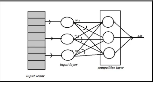
a. LVQ Architecture:
As the neural net of LVQ is a supervised network each of its output unit is referred as a class and represents competitive network architecture.
Figure 1. LVQ Architecture.
Steps for Initializing reference vector
a) Take first d training vectors and use them as weight vectors, the remaining vectors are used for training. b) Initialize the reference vectors randomly and assign
the initial weights and class randomly.
b. Training Algorithm:
Step 1:Initialization of weight (reference) vectors. Initialize learning rate.
Step 2:While stopping is false, do step 3-7.
Step 3:For each training input vector x, do steps 4-5. Step 4:Compute j using squared Euclidean Distance.
D (j) =∑ (wij − xi) 2 (1)
Find J when D (j) is minimum. Step 5:Update wJ as follows.
If t = cJ, then WJ (new) = wJ (old) + α[x − wJ (old)] (2)
If t ≠ cJ, then WJ (new) = wJ (old)−α[x − wJ (old)] (3)
Step 6:Reduce the learning rate. Step 7:Test for stopping condition.
The main objective of LVQ neural net is to find a matching pattern between the input and the output vectors. At the end of the process if input x and weight w belong to same class then the weights are moved toward the new input vector else they are moved away from the input vector. The winner unit index is compared with the target and based upon its result the weights are updated.
C. Multilayer Perceptron Model (MLP):
Perceptron is a computational model of the retina of the eye and hence is named perceptron. This network comprises of three units [3]:
a) Sensor unit (S) b) Association unit (A) c) Response unit (R)
Figure 2. Perceptron Model.
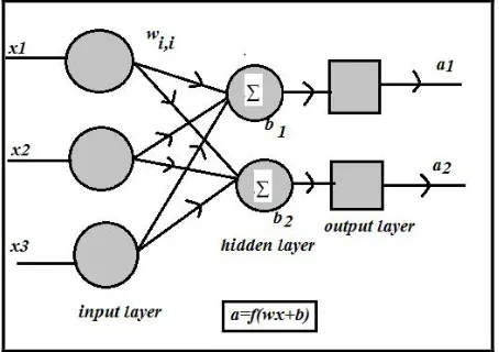
Multilayer Perceptron model (MLP) is a feed-forward neural network with dedicated input and output layers. It consists of a set of sensory units that constitute the input layer and one or more hidden layer of computation modes. A network of this type is called MLP.
Figure 3. Multilayer Perceptron.
III. LITERATURESURVEYONCLASSIFICATION
Previously many works have been done regarding finding out the diseased heart accurately.
a. One of the works includes classification of the patients into number of attacks depending on a set of 13 attributes using Linear Vector Quantization in neural networks [12].
b. The other includes classification of heart into healthy or weak depending on the same set of attributes and implanting it through the Multi-Layer Perceptron (MLP) model [1].
c. In this paper we use the heart disease data along with its attributes.
A. Description of Data:
We have taken the heart disease data set from Cleveland Clinic Foundation database, supplied by Robert Detrano, M.D., Ph.D. This dataset was collected by David Aha and given at UCI machine learning repository, Center for machine learning and intelligent systems [14][15]. In this data set 14 attributes were recorded after various medical tests. It concerns classification of person into normal and abnormal person. The initial 13 attributes were numerical values like age, sex, cp etc. and the 14th attribute contains 4 values. ‘0’ for normal person, ‘1’ for first stroke, ‘2’ for second stroke, and ‘3’ for end of life. We can use this data together with one of more data mining techniques to help us develop profiles for differentiating individuals with heart disease from those without known heart conditions.
Table I. Attribute Description
Attribute Description Range Age (1=Typical angina; 2= Atypical angina;
3=Non-anginal pain; 4= Asymptotic) abnormality; 2= probable or definite
Hypertrophy) Exercise induced angina(1=yes;0=no)
Numeric
(1=up; 2=flat; 3= down)
Number of major vessels (0-3)
Normal, fixed defect, reversible defect
Continuous
Above 13 attributes are recorded after Heart diagnosis.
B. Classification Using LVQ [2][12]:
Linear vector quantization (LVQ) is one of the best in pattern classification in the field of neural networks when compared to Hebb net, Perceptron or ADALINE networks. Linear Data Scaling: Here each input data is converted into the range between 0 to 1 using the formulae given below. Delta = Xmax− Xmin (4) but, 0.1 is taken for which maximum efficiency was obtained [2]. The experimental results are shown and compared in section V.
C. Classification using MLP [1]:
Anchana Khemphila and Veera Boonjing from the Department of Mathematics and Computer Science Faculty of Science, King Mongkut’s Institute of Technology Ladkrabang have adopted the Multi-layer Perceptron model in order to classify the patients into healthy or affected heart.
Multilayer is feed-forward neural networks trained with the standard back propagation algorithm. It is supervised networks so they require a desired response to be trained. It learns how to transform input data in to a desired response, so they are widely used for pattern classification. With one or two hidden layers, they can approximate virtually any input-output map. They performed their experiments and concluded the results with the WEKA 3.6.4 tool and adopted an accuracy formula. This formula uses the Confusion matrix.
Mapping between Actual class & Predicted Class. Accuracy = (n0, 0 + n1, 1) ∕ n (8) Where, n0, 0 is number of C0 cases classified correctly and
n1, 1 is number of C1 cases classified correctly. The
experimental results are shown and compared in section V.
IV. MODIFIEDLINEARVECTORQUANTIZATION
METHOD
method in both the training input vectors and testing input vectors. Many data mining and pattern recognition tasks involve calculating abstract "distances" between items or collections of items.
The Euclidean distance is the geometric distance within 3 spatial dimensions. The Euclidean distance is simple to calculate: square the difference in each dimension (variable), and take the square root of the sum of these squared differences.
A. Drawback of Euclidean Distance:
This distance measure has a straightforward geometric interpretation, is easy to code and is fast to calculate, but it has two basic drawbacks [16]:
a. The Euclidean distance is extremely sensitive to the scales of the variables involved. Modelling problems might deal with variables which have very different scales, such as age, height, weight, etc. The scales of these variables are not comparable.
b. It is blind towards the duplicated variables, and treats it as new information. It weights the copied variable more heavily in its calculations than the other variables.
B. Mahanalobis Distance:
Mahalanobis distance takes into account the covariance among the variables in calculating distances. With this measure, the problems of scale and correlation inherent in the Euclidean distance are no longer an issue [16].
Consider 2 multivariate vectors X = (x1, x2, x3… xn) t and Y = (y1, y2, y3… yn) t and their covariance matrix S, then the Mahalanobis Distance is given by:
DM (x) = √ [(x − y) t S-1(x − y)] (9)
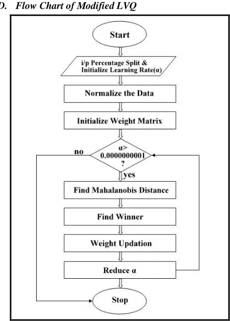
C. Modified LVQ Algorithm:
The algorithm is as follows:
Step 1:Initialization of weight (reference) vectors. Initialize learning rate.
Step 2:While stopping is false, do step 3-7.
Step 3:For each training input vector x, do steps 4-5. Step 4:Compute j using squared Mahalanobis Distance.
DM (j) = (x − w) t S-1(x − w) (10)
Find J when DM (j) is minimum. Step 5:Update wJ as follows.
If t = cJ, then WJ (new) = wJ (old) + α[x − wJ (old)] (11)
If t ≠ cJ, then WJ (new) = wJ (old)−α[x − wJ (old)] (12)
Step 6:Reduce the learning rate. Step 7:Test for stopping condition.
D. Flow Chart of Modified LVQ
Figure 4. Modified LVQ flow chart.
V. EXPERIMENTALRESULTS&DISCUSSION
The main objective of modified LVQ algorithm was to improve the efficiency of the classifier as compared to previously developed classification algorithms, like, LVQ and MLP.
The algorithm was implemented using MATLAB 2007b, taking into account the percentage split of training input vectors and testing input vectors from the predefined dataset.
A. Results of classification using MLP:
Sample heart data -
The given dataset was split into 40% as training vector and rest 60% was used for testing. The results of confusion matrix and accuracy calculation (Using formula specified above) are given below:
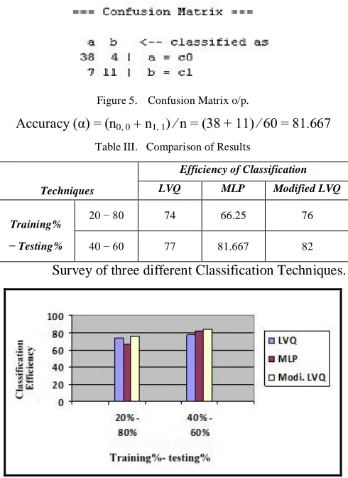
Figure 5. Confusion Matrix o/p.
Accuracy (α) = (n0, 0 + n1, 1) ∕ n = (38 + 11) ∕ 60 = 81.667
Table III. Comparison of Results
Techniques
Efficiency of Classification
LVQ MLP Modified LVQ
Training%
− Testing%
20 − 80 74 66.25 76
40 − 60 77 81.667 82
Survey of three different Classification Techniques.
Figure 6. Efficiency Comparison Graph.
The above table (see Table III) and graph (see Figure 6) gives a complete demonstration of the efficiency of classification of the various techniques employed for classifying heart disease patient’s database.
VI. CONCLUSION
In the above study we emphasised on different classification techniques for classifying the heart disease dataset. Here we showed a parallel comparison between LVQ, MLP and Modified LVQ classification techniques focusing mainly on their efficiency of classification. From the above tabulation we can conclude that more the percentage of training vectors of the dataset more is the efficiency of the system. We also came to know in case of distance calculation method Mahalanobis distance is more accurate than Euclidean distance as it takes into account the covariance of the input variables.
Here we conclude that for a given heart disease dataset with 40% of it taken as training vector and the rest 60% as testing vector LVQ shows an accuracy of 77%, while MLP
shows an accuracy of 81.667% and at the same time
modified LVQ shows an efficiency of 84% (see Table III).
VII. REFERENCES
[1] Anchana Khemphila and Veera Boonji, “Heart disease Classification using Neural Network and Feature Selection”, IEEE DOI 10.1109/ICSEng.2011.80.
[2] Dr. K. Usha Rani, “Analysis of heart diseases dataset using neural network approach”, International Journal of Data Mining & Knowledge Management Process (IJDKP) Vol.1, No.5, September 2011.
[3] S.Rajasekharan and G.A.Vijayalakshmi Pai “Neural networks, fuzzy logic and genetic algorithms synthesis and applications”.
[4] A. Kusiak, K.H. Kernstine, J.A. Kern, K A. McLaughlin and T.L. Tseng, “Data mining: Medical and Engineering Case Studies”, Proceedings of the Industrial Engineering Research Conference, Cleveland, Ohio, May21-23, 2000, pp.1-7. [5] H. B. Burke, “Artificial neural networks for cancer research:
Outcome prediction,” Sem. Surg. Oncol., vol. 10, 1994, pp. 73–79.
[6] H. B. Burke, P. H. Goodman, D. B. Rosen, D. E. Henson, J. N. Weinstein, F. E. Harrell, J. R. Marks, D. P. Winchester, and D. G. Bostwick, “Artificial neural networks improve the accuracy of cancer survival prediction,” Cancer, vol. 79, 1997, pp. 857–8621997.
[7] Siri Krishan Wasan1, Vasudha Bhatnagar and Harleen Kaur, “The impact of Data Mining Techniques on Medical Diagnostics”, Data Science Journal, Volume 5, 119-126, 2006.
[8] R. Scales, R., & Embrechts, M., “Computational Intelligence Techniques for Medical Diagnostic”, 2002, Proceedings of Walter Lincoln Hawkins, Graduate Research Conference from
the World Wide Web: http://www.cs.rpi.edu/~bivenj/MRC/proceedings/papers/resea
rchpaper.pdf.
[9] S. M. Kamruzzaman, Md. Monirul Islam, “An Algorithm to Extract Rules from Artificial Neural Networks for Medical Diagnosis Problems”, International Journal of Information Technology, Vol. 12 No. 8, 2006.
[10]Hasan Temurtas, Nejat Yumusak, Feyzullah Temurtas, ” A comparative study on diabetes disease diagnosis using neural networks”, Expert Systems with Applications: An International Journal, Volume 36 Issue 4, 2009.
[11]O. Er, N. Yumusak and F. Temurtas, "Chest disease diagnosis using artificial neural networks", Expert Systems with Applications, Vol.37, No.12, 2012, pp. 7648-7655.
[12]S N Sivanandam, S Sumathi and S N Deepa “Introduction to neural networks using MATLAB 6.0”.
[13]Jamal M. Nazzal, Ibrahim M. El-Emary and Salam A. Najim, “Multilayer Perceptron Neural Network (MLPs) For Analyzing the Properties of Jordan Oil shale”. World Applied Sciences Journal 5 (5): 546-552, 2008.
[14]David Aha “Heart Disease Dataset” http://archive.ics.uci.edu/ml/datasets/Heart+Disease.
[15]Kurgan, Lukasz A., Cios, Krzysztof J., Tadeusiewicz, Ryszard, Ogiela, Marek, & Doodenday, Lucy S., “Knowledge discovery approach to automated cardiac SPECT diagnosis.” Artificial Intelligence in Medicine, 149169, 2001.
[16]Will Dwinnell,