Performance Evaluation and Rate of Acceptance of Various Multistage Interconnection Networks

(1)

!

"

# #

"$ % %#

&

''' (

Performance Evaluation and Rate of Acceptance of Various Multistage Interconnection

Networks

Lovnish Bansal* and ShrutiGoel

CSE Department, Bhai Maha Singh College of Engg. Muktsar (Punjab) India

[email protected], [email protected]

Abstract

:

This paper states the various methods to evaluate performance of various Multistage Interconnection Networks. A number of

Interconnec-tion Networks are studied to get the most reliable network. We have implemented three different algorithms to find the reliability of a network and to get the probability of acceptance of a Multistage Interconnection Network. We also come to the conclusion that the Irregular Multistage tion Networks are more reliable than Regular Multistage Interconnection Network because the number of stages in Irregular Multistage Interconnec-tion Networks are lesser than that of Regular Multistage InterconnecInterconnec-tion Networks .

A Number of Performance factors are used like Bandwidth, Probability of Acceptance and cost of regular and irregular interconnection networks. We will also compute reliability of various Multistage Interconnection Networks with and without repairing of switching elements.

Keywords:Multistage Interconnection Network, Bandwidth, Performance, Reliability, Switching elements.

I. INTRODUCTION

Multistage interconnection network is a set of connections between multiprocessor systems, ATM switches, or Gigabit Ethernet switches. And each Switch is a cross bar Network. Various types of Regular and Irregular Multistage Intercon-nection networks are:-

a) Omega Network

b) Augmented Shuffle Exchange Network c) Augmented Baseline Network

d) Zeta Network

[image:1.612.326.576.333.395.2]

A Multistage Interconnection Network consist of number of stages as shown in Fig.1.

Fig.1 Multistage Interconnection Network

The main objective of Interconnection Network is to de-sign a network that combines full connection capability with graceful degradation in spite of the existence of faults.

[image:1.612.48.266.500.588.2]

A switch in Multistage Interconnection Network can work in either T-mode to provide parallel connection or in X-mode to provide cross connection as shown in Fig.2.

Figure 2 T-mode and X-mode of Switch

Various Connection Issues in Multistage Interconnection Networks are Bandwidth, Probability of acceptance, Through-put, Reliability, Permutation, Cost, Path length, Fault tolerance and performance. Reliability of an Interconnection Network can be measured in two ways:-

a) Series Reliability Model b) Parallel Reliability Model

A. Series Reliability model

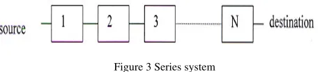
A system is said to be in series if all the component of this are involved during the operation. The failure of any compo-nent means failure of the whole system. Reliability of a series type of system is shown in Fig.3.

Figure 3 Series system

It is given by the product of reliabilities of individual component in it.

R

SERIES

(t) = P

1

(t) . P

2

(t) . P

3

(t)……P

n

(t) = P

i

(t)

[image:1.612.333.561.573.625.2]

(2)

B. Parallel Reliability Model

[image:2.612.51.274.115.219.2]

A system is said to be in parallel if the successful func-tioning of any of the component leads to the success of the system. System fails only when the entire component fails.

Figure 4 Parallel System

Reliability of a parallel type of system is given by

R

parallel

(t) = 1- (1-P

i

(t))

Where Pi is the reliability of IN component.

We can classify Multistage Interconnection Networks (MINs) as:-

a) Unique Path MINs b) Multi-path MINs c) Regular MINs d) Irregular MINs e) Static MINs f) Dynamic MINs

a) Unique Path MIN: - Unique paths MINs are characterized by the presence of single unique path between any source des-tination pair.

b) Multi-Path MIN: - The multiple paths between each input-output pair of the network are provided by connecting switch-ing elements within the same stage. This technique is called chaining. The chained network possesses alternate paths that are available at each switching element, thus the network is strongly re-routable.

c) Regular Network: - Any network is said to be regular if the number of switching elements (SEs) in different stages of the network is same.

d) Irregular Network:- Any network is said to be irregular if the number of switching elements (SEs) in different stages of the network is different.

e) Static Interconnection Network: -In a static interconnection network, links among different nodes of system are passive. f) Dynamic Interconnection Networks:Dynamic networks are built using switches and communication links.

II. METHODOLOGY

A. Omega Network

The Omega network is one particular kind of multistage network; it is a unique path interconnection network which provides a distinctive path between any input and output. Omega Network has N = 2n inputs, termed sources (S), and 2n outputs termed destinations (D). There is a unique path be-tween each source-destination pair. The Omega Network has n stages and each stage has N/2 switching elements. The

net-work complexity, defined as the total number of switching elements in the MIN, is (N/2)(log2 N).

Each stage implements a perfect shufflewire interconnec-tion followed by N/2 switching elements, where each switch is capable of sending either input to either output. It is assumed that each input to a switch can receive at most one input, and that the switches do not contain queues. For presentational convenience, it is assumed that a switch cannot send a given input to both outputs, but the results do not depend on this assumption. In Fig. 5, various interconnection links for each stage from the top down with an N-bit binary address, and have been labeled shown with two paths through the network.

Figure5 8X8 Omega Network

B. Routing in Omega Network

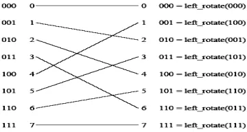
Let Sm-1,Sm-2,...,SO and dm-l,dm-2,...,do be the binary repre-sentations of the source and destination addresses respectively, where mis the number of address bits (m = log2n).The switch-es along the path in stage i use the bit dm-iand make a connec-tion to the upper output link if the bit is 0 or to the lower out-put link if it is 1. Fig.6 shows how a cell is routed form S2 to

[image:2.612.334.558.491.605.2] [image:2.612.340.520.632.728.2]

D4. Routing is represented as the bitwise shuffle-exchange shown in Fig. 7. The resulting address after a shuffle corres-ponds to the switch input at each stage, and the resulting ad-dress after an exchange corresponds to the switch output at each stage. A complete routing requires m shuffle-exchanges until the packet reaches its destination. The address labels in Fig.7 shows an example of this operation.

Figure 6 Shuffle Exchange in Omega Network

(3)

C. Performance Analysis

Assume a MIN of size an bn constructed from a b

crossbar switches and having an Sources connected to destina-tions. The analysis of crossbar is applied to a b crossbar switch and then extended to the complete MIN. The distinct destination digit (in base b) for setting of individual a b switches controls each stage of MIN.

The probabilistic approach is used to analyze the MINs based on independent request assumptions. Given the request rate p at each of the a inputs of an a b crossbar module, the ex-pected the rate of requests on any one of the b output lines from any one input is given by p/b.

Probability of not getting the request is:

1 – p / b

Probability of not getting the request from all ‘a’ inputs is giv-en by:

(1 – p / b)

a

Probability of one output getting the request from all ‘a’ inputs is given by:

1-(1 – p / b)

The total number of requests that it passes per unit time is giv-en by

b- b(1-p / b)

a

Since the output rate of a stage is the input rate of the next stage, output rate of any stage can be recursively calculated starting from stage 1and the output rate of final stage n deter-mines the bandwidth of MIN

D. Probability Equations for Omega Network

Probability equations for 16 × 16 Omega Network is giv-en by:

p0 = p p1 = 1- ( 1 –p0 /2 ) 2 p2 = 1- ( 1 –p1 /2 ) 2 p3 = 1- ( 1 –p2 /2 ) 2 p4 = 1- ( 1 –p3 /2 ) 2

pn = p4

E. Reliability Analysis

Reliability of the network is concerned with the ability of a network to carry out its desired network operation success-fully. Reliability of a system is the probability that it will per-form its intended function satisfactorily for a given time under stated operating conditions. These networks are able to send messages through alternative paths when some faults are de-tected in the regular route. This reliability measure is some-times referred to as the Source-to-Multiple Terminal (SMT) Reliability.

The reliability measures of particular interest are:

• Terminal Reliability (TR)

• Broadcast Reliability (BR)

• Network Reliability (NR).

a) Terminal Reliability (TR):Terminal reliability, generally used as a measure of robustness of a MIN, is the probability of existence of at least one fault free path between a designated pair of input (s) and output (t) terminals (two-terminal).

b) Broadcast Reliability (BR) Another useful measure of the reliability of a MIN is its ability to broadcast data from a given input terminal to all the output terminals of the network. A network is said to have failed when a connection cannot be made from the given input terminal to at least one of the out-put terminals.

c) Network Reliability (NR): The network reliability is de-fined as the probability that there exists a connection between each input to all outputs (all-terminal).

We have made some assumptions to calculate reliability using Markov Model:-

1) All SEs are substantially less reliable than the links. The SEs is dynamic solid-state devices that have a calculable im-perfect reliability. Links are typically static devices such as backplanes or wires.

2) Each SE in the MIN has two states: good or bad.

3) The reliability of the SE is known. With a given (t),using the exponential model one can compute the reliability pi of the

SE as:

4) When X (t) is constant, then:

5) The SEs can be repaired.

6) Allfailures are statistically-independent i.e. All the switch element are not depend on each other. 7) The failure of switch occur independently in a network with a failure rate of (= 10

-6

per hour) pre unit time. Based on the gate count failure rate for 2×2 SE, 2= and for 3×3 SE 3 = 2.25 , for m: 1

multip-lexer m = d = /4×m = failure rate of 1: m demultiplexer.

Now we can obtain the time-dependent reliability of PC by symbolically this 3-state Markov model:

(1)

R

PC

(t) = Be

- t

+ Ce

- t

(2)

1

3

2

(

8

2

)

2

c

α

=

µ

+

λ

−

µ

+

λµ

−

+

λ

(3)

(

)

2 2

1

3 8 2

2 c

β = µ + λ + µ +λ µ − +λ

(4)

1 ₍ ₂ ₍ _{1) )}

B

β

λ

C

β

α

= + −

−

(5)

1 ₍ ₂ ₍ _{1) )}

C = −

β

α

+

λ

C −

−

MTTF (Mean Time To Failure)

The mean time to failure is the integral under the reliability curve.

0

( )

MTTF

R t dt

∞

=

F. Reliability of Omega Network

(4)

any of the switching elements, multiplexers or de-multiplexers may fail.

The analysis is carried as under:

Let Rs (t), the reliability function of a component, be defined

as the probability that a failure does not occur in the time pe-riod (0,t).

Reliability of Omega Network is:-

R(t)

omega

= [e

t

]

N/2*log2N

0 0 .0 5 0 .1 0 .1 5 0 .2 0 .2 5 0 .3

4 1 6 64 2 56 1 0 24

R e li a b ili ty

ne tw ork s iz e

R elia b ili ty o f o m eg a n et w o rk

Figure 8 Reliability of Omega Network

MTTF is dependent on the network size N and on the real time operation‘t’. By using 2x2 switching element MTTF for Omega network is evaluated from the following expression.

x

MTTF

omega

= [e

- t

]

N/2*log2N

* dt

0

Table I. Reliability of omega network for different size of networks

NETWORK SIZE

Reliability (MTTF * )

4 0.25000

8 0.08333

16 0.03125

32 0.01250

64 0.00520

128 0.00260

256 0.00097

512 0.00004

1024 0.00019

G. Shuffle Exchange Network (SEN)

SEN is a unique-path MIN, the failure of any switch causes system failure, so from the network reliability point of view, we have (N/2)(log2N) SEs in “series”. Thus, imperfect

coverage and repair are not factors in the computation of sys-tem reliability. Assuming a constant failure rate for each com-ponent, let 2 denote the failure rate of SE2.

Hence, the time-dependent reliability and the mean time-to-failure of an N× N SEN is given by:

2 2

1 _{l o g} 2

( ) t N N

S E N t

e

R

−λ

=

2

1 _{lo g}

2

1

N

S E N _N

M T T N

=

Extra Stage Shuffle Exchange Network (SEN+)

Exact reliability analysis of the SEN+, even with perfect cov-erage and no repair, becomes intractable for networks larger than 16×16. However, useful lower and upper bounds have been derived. We extend these reliability bounds to incorpo-rate imperfect coverage and repair. By applying the composi-tion of the subsystems as illustrated with the 2-component parallel system, we can determine the reliability and availabili-ty expressions.

H. Pessimistic (lower bound) analysis of SEN+

The switching elements in the intermediate stages of a SEN+ can be failed, and yet the network is still operational. We model the intermediate stages as a system consisting of a parallel arrangement of two series subsystems each with (N/4) (log2 N - 1) switches. We have a series system of three

subsys-tems-the first and last are series subsystems and the middle subsystem is a parallel-series subsystem.

The reliability expression using lower bound is given by

' '

2 2 2

( ) [ ' ' ]

L B

N t t t K

S E N t e B e C e

R

− λ −α −β

+ = +

The Mean Time to Failure is:

Where B’, C’, ’, ’ are determined by substituting ¼ N(log2N-1) 2 for inn equations (2) to (5).

I. ASEN-2Network

Augmented Shuffle Exchange Network (ASEN-2) is a regular network, having equal number of switches in each of the stage. ASEN-2 network is constructed from Shuffle Ex-change Network by adding a stage of 2×1 multiplexers at the initial stage and 1×2 demultiplexers at last stage. It provides multiple paths between a source and a destination. ASEN-2 of size N × N with N number of sources and N number of desti-nation consists of log2N -1 stages where the initial stage con-sists of N/2 switches of size 3×3 and the last stage consist of N/2 switches of size 2×2.

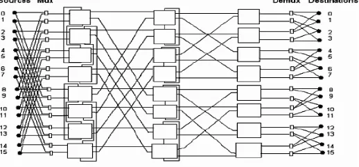
ASEN-2 provides fault tolerance using links between the con-jugate pairs of switches. A 16×16 ASEN- 2 network is shown in Fig.9.

' '

2 2

' '

L B

S E N

M T T F

N N

B C

α λ β λ

[image:4.612.34.285.148.303.2]

(5)

[image:5.612.45.304.58.179.2]

Figure 9 Augmented Shuffle Exchange Network(ASEN-2)

The reliability expression using lower bound is given by:

( ) ( ) ( )

1

3 3 3 3 2 2

0 0 0

! ! !

( ) [( ) ( ) ( ) ( ) ( ) ( ) ]

! ! ! ! ! !

lb

I J K

i i j J j k K k

ASEN m m m m

i j k

I J K

R t B C B c B C

i I i j J j k K k

− − −

= = =

= ×

− − −

×exp[ {−iα₃m+(I i−)β₃m+jα₃+(J−j)β₃+kα₂m+(K k− )β₂m} ]t

Where Bm,Cm, m, m are determined by substituting m for ;

B3,C3, 3, 3 are determined by substituting 3 for ; and

B2m,C2m, 2m, 2m are determined by substituting 2m for in

above equation, respectively I= N/2, J=N/4×(n-2) and K=N/4 where n=log2N.

The mean time to failure is given by:

( ) ( )

(

)

0 0 0

! ! !

( )

! ! ! ! ! !

u b

I J K

A S E N

i j k

M T T F t I J K

i I i j J j k K k

= = =

×

=

− − −

1

3 3 2 2

[ ( ) ( ) ( ) ( ) ( ) ( ) ]

( ) ( ) ( )

j J j

i i k K k

m m m m

B C B c B C

iα I i β jα J j β kα K k β

−

− −

+ − + + − + + −

J. Augmented Baseline Network (ABN)

Exact reliability analysis of the ABN, even with perfect coverage and no repair, is tractable only for rather small (8×8) networks. For larger networks, useful lower and upper bound RBD models were initially proposed; these RBD models were extended to incorporate the added complexity of the SEs used in the ABN, the multiplexers and demultiplexers used at the input and output interfaces of the network, and preliminary reliability analysis which separately considered on-line repair and imperfect converge was presented.

We considered the 2×2 switch and its associated demultiplex-ers as a single component (SE2d), so 2d =2 can be assigned to

this group of elements. Also let 3 be the failure rate for the

3×3 switch (SE3), then based on gate count 3 = 2.25 and

aggregated failure rate will be 3m = 4.25 .

K. Optimistic (Upper bound) analysis of ABN

To obtain an upper bound for the ABN, we observe that each source is connected to two multiplexers and each SE has a conjugate. So if we assume that the ABN is operational as long as one of the two multiplexers attached to a source is operational and as long as both components in a conjugate pair are not faulty, then we will permit as many as one-half of the system components to fail and the ABN can still be operation-al reliability block. The upper bound of the ABN reliability is:

( )

(

)

1

3 3 2 2

0 0 0

!

()

[( )( ) ( ) ( ) ( ) ( ) ]

!

! !

!

ub

I J K

i i j J j k K k

ABN m m d d

i j k

I

J

K

R t

B C B c

B C

i I i

j J j

k K k

− − −

= = =

=

×

−

×exp[ {−iαm+(I−i)βm+jα₃+(J−j)β₃+kα₂d+(K−k)β₂d} ]t

(

)

(

)

(

)

0 0 0

!

( )

!

ub

I J K

ABN

i j k

MTTF

t

I

J

K

i I i

j J

j

k K k

= = = ×

=

−

1

3 3 2 2

[( ) ( ) ( ) ( ) ( ) ( ) ]

( ) ( ) ( )

j J j

i i k K k

m m d d

B C B c B C

−

− −

+ − + + − + + −

Where Bm, Cm, m, m are determined by substituting m for .

B3,C3, 3, 3 are determined by substituting 3 for ; and

B2d,C2d, 2d, 2d are determined by substituting 2d for in

above equation, respectively I= N/2, J=N/4×(n-3) and K=N/4. Probability Equations for Augmented Baseline Network

Probability equations for 16 × 16 Augmented Baseline Net-work are given by:

p0 = p

p1 = 1- ( 1 –p0 /3) 3

p2 = 1- ( 1 –p1 /2 ) 2

L .Pessimistic (lower bound) analysis of ABN

At the input side of the ABN, the multiplexers are not considered an integral part of a given 3×3SE. That is, a mul-tiplexer can be failed, and as long as at least one of its two associated SEs is operational, the network can be operational. But if we group two multiplexers with each SE on the input side and consider them as a series system, then we have a con-servative estimate of the reliability of these three components. Finally, these aggregated components and the SEs in the in-termediate stages can be arranged in pairs of conjugate loops. To obtain the pessimistic (lower) bound on the reliability of the ABN, we assume the network is failed whenever more than one loop has a faulty element or more than one SE in a conju-gate pair in the last stage fails. The ABN can tolerate any sin-gle loop failure or the failure of any sinsin-gle switch in the last stage.

For N 8, the lower bound of the ABN is:

( )

(

)

(

)

1

3 3 3 3 2 2

0 0 0

! ! !

() [( )( ) ( ) ( ) ( ) ( ) ]

! ! ! ! ! !

lb

I J K

i i j J j k K k

ABN m m d d

i j k

I J K

R t B C B c B C

i I i j J j k K k

− − −

= = =

= ×

− − −

3 3 3 3 2 2

exp[ {iαm (I i)βm jα (J j)β kαd (K k)βd} ]t

× − + − + + − + + −

(

)

(

)

(

)

0 0 0

! ! !

( )

! ! ! ! ! !

lb

I J K

ABN

i j k

I J K

MTTF t

i I i j J j k K k

= = =

×

=

− − −

1

3 3 3 3 2 2

[( ) ( ) ( ) ( ) ( ) ( ) ]

( ) ( ) ( )

j J j

i i k K k

m m d d

B C B c B C

−

− −

+ − + + − + + −

Where B3m, C3m, m, m are determined by substituting 3m for

. B3,C3, 3, 3 are determined by substituting 3 for and

B2d,C2d, 2d, 2d are determined by substituting 2d for in

(6)

M. Calculation of Bandwidth and Probability of Acceptance

Bandwidth in computer networking refers to the data rate supported by the network connection or interface. One most commonly espresses bandwidth in terms of bits per second (bps.), the terms comes from the electrical engineering, where bandwidth represents the total distance or range between the highest or lowest signals on the communication channel (Band).

Bandwidth represents the capacity of the connection. The greater the capacity, the more likely that greater performance will be.

Above given probabilistic equations are utilized for the pur-pose of achieving some analytical results. So Bandwidth BW is given by: -

BW = p[n] × Size of the Network

Probability of acceptance (Pa) is defined as the ratio of ex-pected bandwidth to the exex-pected number of request generated by a source per cycle.

III RESULTS AND DISCUSSIONS

A. Cost Effectiveness

To estimate the cost of a network, one common method is to calculate the switch complexity with the assumption that the cost of a switch is proportional to the number of gates in-volved, which is roughly proportional to the number of cross points within a switch. For example 2×2 switch has 4 units of hardware cost, where as 3×3 has 9 units for the multiplexer and de-multiplexers. We roughly assume that each of m×1 multiplexer or 1×m de-multiplexer has m units of cost.

0 0 .0 1 0 .0 2 0 .0 3 0 .0 4 0 .0 5 0 .0 6 0 .0 7 0 .0 8 0 .0 9

0 .0 2 0 .0 4 0 .0 6 0 .0 8

R e li a b il it y

F a il u r e R a te

u b ( S E N + ) l b( S E N + ) u b ( A S E N ) l b( A S E N ) u b ( A B N ) l b( A B N )

Figure 10 Reliability Comparison between SEN+, ASEN and ABN Networks

Comparison of Reliabilities between SEN+, ASEN and ABN with perfect convergence and no repair.

Fig.10 shows the comparison of reliabilities between SEN+, ASEN and ABN with convergence and no repair.

Table 3. below shows the comparison of bandwidth of various MINs.

Table II. Networks with their cost functions

NETWORK COST

ESC 2N(log2N +C)

ASEN 3N(1.5 log2N-1)

ABN (9 log2N-11)N/2

ZTN N/8(56+24 log2(N/2))

[image:6.612.317.569.130.257.2]

MFT-New 2N(log2N+5)+N/2

Table III. Comparison of Bandwidth between Omega, ASEN, ABN and MFT-New network

P OMEGA ASEN ABN MFT-New

0.1 1.45 1.46 1.51 1.42

0.2 2.64 2.69 2.85 2.55

0.3 3.63 3.71 4.04 3.46

0.4 4.45 4.58 5.09 4.20

0.5 5.13 5.31 6.03 4.81

0.6 5.71 5.92 6.85 5.31

0.7 6.17 6.45 7.58 5.73

0.8 6.57 6.9 8.22 6.08

0.9 6.92 7.28 8.78 6.38

IV CONCLUSION AND FUTURE SCOPE

• Irregular MINs are better than that of Regular MINs in terms of reliability.

• It is concluded that the performance of MINs with repair of switching elements is better than without repair (in terms of Reliability) on various MINs.

• Reliabilty of Multipath MIN’s is more then Unique path MIN’s. i.e Reliability of SEN+ is More then SEN with and without repair.

• As the Network size increases, Reliability in terms of MTTF of the MINs Decreases.

• Probability of Acceptance decreases as request generation probability increases.

• Irregular MINs are more Cost Effective as compared to regular MIN’s.

Future Scope

• Reliability analysis can also be done of Optical MINs.

• By using Markov Model Availability analysis can be done for various types of regular and irregular MINs.

• The detailed Performance analysis can be done for vari-ous MINs by using other parameters Throughput, Permu-tation Possibility, Latency and Path length etc.

• A comparative analysis of irregular MINs with the regular MINs can be done by using another performance parame-ter.

V. REFERENCES

[1] Sheta, Parameter Estimation of Software Reliability Growth Models by Particle Swarm Optimization, ICGST-AIML Journal, Vol. 7, No.7, June,2007, pp.55-61.

[2] H. Aggarwal, and P.K. Bansal, Routing and Path Length Algorithm for cost effective Modified Four Tree Network, IEEE TENCON, 2002, pp. 293-294.

[image:6.612.34.292.415.553.2]

(7)

Applications,Gold Coast, Australia, Jan, 2007, pp. 17-19.

[4] J. Sengupta and P.K Bansal, “Reliabilty and perfor-mance measures of regular and irregular Multistage Interconnection Networks”, Interational Conference IEEE TENCON 2000, pp. 531-536.

[5] J. Sengupta and P.K. Bansal, “Performance Analysis of Regular and Irregular Dynamic MINs”, Interna-tional Conference IEEE TENCON 99, Sept. 1999, Cheju Island, Korea, pp. 427-430.

[6] Jose Duato, Sudhakar Yalamanchili and NiLionel, “Interconnection Networks: An Engineering Ap-proach”, IEEE Computer Society, 1997.

[7] M. Lubazewski and B Coutois, ”A Reliable Fail-safe System”, Parallel and Distributed Systems, IEEE Computer Society, Vol. 47, No. 2, Feb. 1998, pp. 236-241.

[8] N Laxmi Bhuyan, Yang Qing and Dharma PAgraw-al., “Performance of Multiprocessor Interconnection

Networks”, IEEE Computer, Vol. 22, Feb. 1993, pp. 25-37.

[9] Nitin, “On analytic Bounds of Regular and Irregular Fault-tolerant Multistage Interconnection Networks”, International Conference on PDPTA, June 2006, pp. 26-29.

[10] V. Cherkassky, E. Opper, and M. Malek, "Reliability and fault diagnosis analysis of fault-tolerant multis-tage interconnection networks," in Proc. Fourteenth Int. Symp. Fault-Tolerant Comput, June 1984, pp. 246-251.

[11] L. Ciminiera and A. Serra, "A fault-tolerant connect-ing network for multiprocessor systems," in Proc. Int. Conf. Parallel Processing, Aug. 1982, pp. 113-122.

[12] R. Das and L. N. Bhuyan, "Reliability simulation of multiprocessor systems," in Proc. Int. Conf. Parallel Processing, Aug. 1985, pp. 591-598.