Superresolution Imaging for Forward-Looking Scanning Radar with Generalized Gaussian Constraint

(1)

Superresolution Imaging for Forward-Looking Scanning Radar

with Generalized Gaussian Constraint

Yin Zhang*, Yulin Huang, Yuebo Zha, and Jianyu Yang

Abstract—A maximum a posteriori (MAP) approach, based on the Bayesian criterion, is proposed to

overcome the low cross-range resolution problem in forward-looking imaging. We adapt scanning radar system to record received data and exploit deconvolution method to enhance the real-aperture resolution because the received echo is the convolution of target scattering coefficient and antenna pattern. The Generalized Gaussian distribution is considered as the prior information of target scattering coefficient in MAP approach for the reason that it could express different target scattering coefficient properties with the control of statistic parameter. This constraint term makes the proposed algorithm useful in different applications. On the other hand, the reconstruction problem can also be viewed as thel_p-norm (0 < p≤ 2) regularization. Simulation results show the robustness of the proposed algorithm against additive noise compared with other superresolution methods.

1. INTRODUCTION

Radar imaging has been widely used in many civilian and military ﬁelds due to its all-weather and day/night ability [1, 2]. High resolution of side-looking and forward-squint imaging of motion platforms have been deeply discussed for many years [3, 4]. However, It is diﬃcult to realize matched two-dimensional resolution in forward-looking region due to the symmetrical and small Doppler bandwidth. This imaging bottleneck seriously restricts the practical applications such as self-landing, navigation, etc.

Many algorithms are proposed for solving this low cross-range resolution problem. The SAR imaging methods have been investigated to realize high cross-range resolution of forward-looking image of this decade, including forward-looking SAR and bistatic SAR [5–8]. The forward-looking SAR employs a uniform array sensors to form the effectiveness second order Doppler phase and solve the ambiguity problem. However, the requirement of setting a large size of array sensors in front of the motion platform influences the stealthiness and maneuverability of airbornes. The bistatic SAR breaks through the limitation of monostatic SAR on forward-looking imaging with appropriate geometry configurations. But the strict geometrical relationship of the two platforms is hardly realized, and the synchronization problem has not be totally solved.

Obviously, realizing high cross-range resolution in forward-looking imaging by SAR techniques will increase the burden and complexity of system and structure. In forward-looking imaging, the scanning radar system which collects received data by a single real aperture antenna or a small size array, is often employed. The beneﬁts of this imaging system include the suitability for any geometry situation, low cost and small size. Although this imaging model obtains low cross-range scanning resolution, we can develop signal processing methods to solve this problem. The clean technique [9–11] and monopulse technique [12–14] are two beam sharpen methods based on scanning radar which could output the high precision of target angle position for single target. However, both of the techniques can not resolve the adjacent targets in one beam. The “clean” algorithm is a classic beam cancellation algorithm

Received 8 December 2015, Accepted 7 January 2016, Scheduled 12 January 2016

* Corresponding author: Yin Zhang ([email protected]).

(2)

2 Zhang et al.

which can be employed to improve the resolution of both the range and cross-range dimensions. But its performance has a obvious degradation when some targets are within one beamwidth. Although improved “clean” algorithms have been proposed, the deconvolution error is hard to eliminate. P´ erez-Mart´ınez et al. developed a Shift-and-Convolution technique for high-resolution radar images with a single realbeam antenna [15, 16]. But this method requires high range resolution, and does not improve the cross-range resolution. Recently, spectrum estimation approaches, including the Scan-MUSIC algorithm and Minimum-Variance beamforming technique have been introduced to improve the cross-range resolution of real aperture radar [17–19]. But the problems of how to obtain enough snapshots for platforms in motion and approaches to improve the computational eﬃciency still remain. In [20, 21], the real iterative adaptive approach (Real-IAA) were introduced to the scanning radar system to enhance the cross-range resolution with only one snapshot.

Bayesian deconvolution is another kind of method which is widely used in radar imaging and detection areas [22, 23]. This method constructs the objective function according to he statistical property of noise and target scattering coefficient distributions. Then reasonable approaches are developed to solve the objective function and obtain the reconstruct result. We introduce this method to forward-looking imaging because the received echo of scanning radar can be regarded as the convolution of target scattering coefficient and antenna pattern [24, 25]. In [24], the Poisson-based maximum a posteriori (MAP) algorithm is proposed based on the assumptions that both of the noise and target scattering coefficient obey independent Poisson statistic. Some references consider different penalty terms in scanning radar imaging for high resolution and denoising [23, 26].

In this paper, we ﬁrst assume the independent complex Gaussian statistic as distribution characteristic of noise. This assumption also could overcome the complex signal deconvolution problem compare with traditional deconvolution approaches. Besides, the Generalized Gaussian distribution is considered as the prior information of target scatters distribution for its wide applicability. It gives us the choice of adopting reasonable prior information when faced with diﬀerent imaging scenes because the statistic property of this distribution is variational by controlling the statistic parameterγ (0< γ≤2). On the other hand, the proposed algorithm can be viewed as the l_p-norm regularization problem. It becomes the sparse signal recovery problem when 0 < p≤1, and the common regularization problem when 1< p≤2.

This paper is organized as follows. The convolution model of forward-looking received signals is analyzed in Section 2. In Section 3, the objective function is established according to the statistic characteristics of noise and target scatters. In addition, the derivation of objective function is given in detail. In Section 4, simulations are provided to verify the performance of the proposed algorithm. Conclusions are given in Section 5.

2. SIGNAL MODEL OF FORWARD-LOOKING SCANNING IMAGING

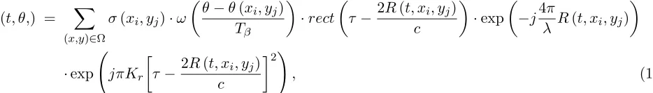
Figure 1 shows the geometric model of the forward-looking scanning radar. The antenna sweeps across the forward-looking scene with counterclockwise mechanical movement. In radar imaging, the −10◦ to 10◦ is often deﬁned as the forward-looking region. The airborne moves along the radial direction with a ﬁxed velocity υ and the platform height is H. Some targets are distributed in the forward-looking imaging region. The antenna transmits linear frequency modulation (LFM) signals for high range resolution. The received signal can be written as the following expression after the antenna scans the whole forward-looking area

s(t, θ,) =

(x,y)∈Ω

σ(x_i, y_j)·ω

θ−θ(x_i, y_j)

T_β

·rect

τ −2R(t, xi, yj) c

·exp

−j4π

λR(t, xi, yj)

·exp

jπK_r

τ− 2R(t, xi, yj) c

2

, (1)

(3)

Figure 1. Geometric model of forward-looking scanning radar.

Figure 2. Range history of antenna and target.

denotes the unit rectangular function; R(t, x_i, y_j) denotes the distance history of scanning antenna and the (x_i, y_j)th target; λ denotes the wavelength of transmitted signal; K_r denotes the chirp rate; c is the speed of light. The original distance between the airborne and the target isR(x_i, y_j), and ϕis the incident angle of antenna. The original distance between the airborne and targetP_i is R0.

Then we take one target in the forward-looking region as an example to analyze the range history. Figure 2 shows the range relationship between airborne and the target located at (x_i, y_j) in the forward-looking area. The range history of airborne and the (x_i, y_j)th target is

R(t, x_i, y_j) = R(x_i, y_j)2+ (υt)2−2R(x_i, y_j) cosθ(x_i, y_j) cosϕυt. (2)

We ﬁnd that the second order term is very small, and the product of time and velocity is also much smaller than the original distance after the Taylor expand of Equation (2). So the range history can be approximately written as

R(t, x_i, y_j) (t)∼=R(x_i, y_j)−cosθ(x_i, y_j) cosϕυt. (3)

We employ pulse compression technique to realize high range resolution because the radar system transmits linear frequency modulation (LFM) signals. For a typical forward-looking radar system, we can construct the range walk correction functionH(f_r, τ) = exp(j2π·f_r·υ_c·τ) to eliminate the inﬂuence of platform movement because the space-variant phenomenon caused by the variety of cross-range angular can be ignored. After these operations, the two-dimensional received signals become

s(θ, τ) =

(x,y)∈Ω

σ(x_i, y_j)·ω

θ−θ(x_i, y_j)

T_β

·sinc

B

τ −2R(xi, yj) c

·exp

−j4π

λR(t, xi, yj)

. (4)

The received signal in Equation (4) has unmatched two-dimensional resolution. In order to improve the cross-range resolution, we ﬁrst rearrange Equation (4) as the following matrix form

s=Wσ+n=

⎡ ⎣

W_N_×_K

. ..

W_M_×_K

⎤ ⎦

⎡ ⎢ ⎢ ⎢ ⎢ ⎢ ⎢ ⎢ ⎣

σ(1,1)

σ(1,2) .. .

σ(1, K) ..

.

σ(N, K) ⎤ ⎥ ⎥ ⎥ ⎥ ⎥ ⎥ ⎥ ⎦

(4)

4 Zhang et al.

where s = [s(1,1), s(1,2), . . . , s(1, M), . . . , s(N, M)]T represents the measurement range profiles which are rearranged in cross-range dimension with size N M × 1; N and M are the sampling numbers of received signal in range and cross-range dimensions, respectively; σ = [σ(1,1), σ(1,2), . . . , σ(1, K), . . . , σ(N, K)]T represents the unknown scene amplitude profiles which are rearranged in cross-range dimension with sizeN K×1;nis the noise vector with dimensionN M×1 which satisfies the complex Gaussian distribution;W is the convolution measurement matrix with size

N M×N K which can be written as

W= [w1,1, . . . , w1,K, . . . , wi,j, . . . , wN,K]T, (6)

and w_i,j is

w_i,j =

a(i,j,1)e(−j

4π

λR(Δt,xi,yj)), . . . , a(i,j,NM)e(−j

4π

λR(NMΔt,xi,yj))

_T

, (7)

where [a₍_i,j,₁₎, . . . , a₍_i,j,NM₎] is the convolution weighted vector of the antenna pattern and the (i, j)th target. (e(−j4λπR(Δt,xi,yj)), . . . , e(−j4λπR(NMΔt,xi,yj))) represent the added phases cause by the relative movement between antenna and the (i, j)th target, and Δtdenotes the pulse repetition interval (PRI). We can develop deconvolution method to reconstruct target scatters distribution in Equation (5).

3. MAP ALGORITHM WITH GENERALIZED GAUSSIAN CONSTRAINT

The proposed Maximum a posteriori (MAP) algorithm is investigated based on the Bayesian criterion. The basic form of MAP estimator is

ˆ

σ= arg max

s p(σ/s) = arg maxs [p(s/σ)p(σ)], (8)

where p(σ/s) is the posteriori probability density function (PDF); p(s/σ) is the likelihood PDF determined by the statistical property of noise;p(σ) is the prior information of target scatters.

In radar imaging, the common hypothesis of noise statistic is Gaussian distribution. Meanwhile, in order to overcome the complex-valued signal recovery problem, we assume that the observed noise obeys i.i.d.complex Gaussian distribution. The likelihood function can be written as

p(σ/s) = 1

(πη2₎MN exp

−1

η2 s−Wσ 2 2

, (9)

whereη2 is the variance of noise. We have mentioned thatp(σ) expresses the prior information of target scatters. In the references, some regularization constraints were considered as the prior information of target scatters. Tikhonov regularization is a commonly used method of regularization of ill-posed problems [27, 28]. The main motivation behind this regularization method lies in replacing the original deconvolution problem with a nearby well-conditioned problem. Another common regularization term is sparse constraint. Recently, the sparse signal recovery problem is deeply discussed in radar imaging when the sampling number or target scatters distribution are sparse. In this paper, we employ the Generalized Gaussian distribution as the prior information for the reason that it can describe as diﬀerent target distribution properties for varying dispersion parameters. The Laplace distribution is often considered as the prior information in Bayesian method which makes the problem can be viewed as the regularized problem with l1-norm constraint after the negative logarithm operation.

However, this prior information only applies to the sparse signal recovery problem. Compared to the Laplace distribution, the Generalized Gaussian distribution can represent diﬀerent constraints, such as Tikhonov regularization and l₁_/₂-norm. It makes the problem can be viewed as the adaptive regularization problem. The Generalized Gaussian distribution function is

p(σ) =

NK

k=1

Ce−|σk|γ/μ₌_CNK_e−NK_k₌₁|σ_k|γ/μ_, ₍₁₀₎

where C is a normalizing constant, γ the dispersion parameter and μ the scale parameter. Using this prior information, the posteriori probability function becomes

p(s/σ)p(σ) = 1 (πη2₎MNe

− 1

(5)

For convenience of calculations, we use the negative logarithm operation to transform the objective function as

−ln (f(s/σ)f(σ)) = M Nlnπη2+_η1₂ s−Wσ2₂−N KlnC+NK

k=1

|σ_k|γ/μ. (12)

Equation (12) shows that the objective function can be viewed as a regularized estimation

problem with variable regularization term NK

k=1

|σ_k|γ/μ. The objective function becomes the Tikhonov regularization when γ = 2, and becomes the classic l1-norm optimization problem whenγ = 1. It can

be viewed as the sparse signal recovery problem when 0 < γ ≤ 1. In practical applications, we often determine this parameter according to the applications and prior information. When this algorithm applies to target location, or the optical image which shows that there only have small number of targets located in the forward-looking region, we can set 0 < γ ≤ 1. If we apply this algorithm to airdrop or know the imaging scene is city, we can set 1< γ≤2 for better image quality and denoising. In order to obtain the iterative expression, we ﬁrst calculate the gradient of Equation (12) with respect to σ as

∇ln (f(s/σ)f(σ)) =WHWσ−WHs+γη

2

μ Gσ, (13)

where (·)H means the conjugate matrix, G = diag{g1, . . . , gNK} and gk = |σk|γ−2. Equation (13) is

minimized when ∇ln(f(s/σ)f(σ)) = 0. The simple optimal solution of Equation (13) is

σ =

WHW+γη

2

μ G

−1

WHs. (14)

Finally, we can get the following iterative formula according to Equation (14) as

σt+1 =

WHW+ γη

2

μ G

t−1_WH_s_, ₍₁₅₎

where t + 1 and t are the iterations, Gt = diag{(g1)t, . . . , (gNK)t} and (gk)t = |(σk)t|γ−2. In

Equation (15), parameter μ is determined by the targets distribution. The noise statistic parameter

η2 can be calculated by the following steps. We minimize Equation (12) with respect to η and set (d/.dη)f(σ, η) = 0 which lead to

η2= 1

M N s−Wσ

2

2. (16)

The coarse noise statistic can be estimated by this equation. We substitute each iterative results of Equation (15) into (16) to continually improve the estimated accuracy ofη2 and σ because small error may cause serious estimation bias. The iterative becomes

σt+1 =

WHW+γ

η2t

μ G

t

₋1

WHs, (17)

where (η2)t = _MN1 s−Wσt2₂. Furthermore, the conjugate gradient (CG) method was employed to realize the matrix inversion for higher computational eﬃciency [29]. This algorithm can also be promoted to other radar imaging ﬁelds.

4. SIMULATIONS

This section compares the performance of proposed deconvolution algorithm with the Real-IAA and Poisson-based MAP deconvolution algorithms.

(6)

6 Zhang et al.

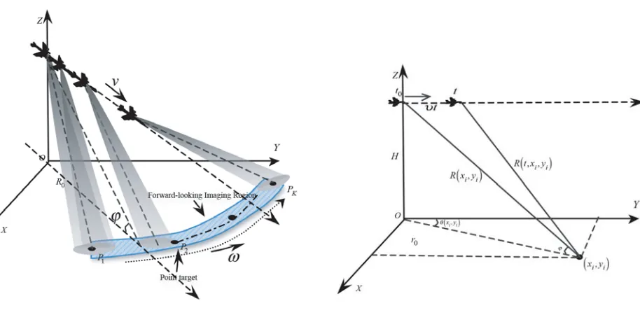
Table 1. Simulation parameters.

Parameter Value Units Carrier frequency 9.6 GHz

Band width 60 MHz Antenna scanning velocity 60 ◦/s

Pulse repetition frequency 1000 Hz airborne height 1000 m Incident angle 30 ◦ Working distance 50 km

airborne velocity 50 m/s

Azimuth dimension (Degree)

Range dimension(Metre)

-5 -4 -3 -2 -1 0 1 2 3 4

4.9 5 5.1 5.2 5.3 5.4 5.5 5.6

x 104

Figure 3. Simulation scene.

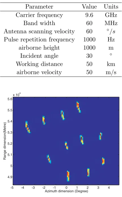
Figures 4 to 6 show the simulation results processed by diﬀerent algorithms when the signal to noise ratio (SNR) is 25 dB. In the simulations, the added noise obeys a zero mean and complex Gaussian distribution, and the SNR is deﬁned as

SN R= 20log₁₀ σ2

σˆ−σ₂. (18)

Figure 4 (a) shows the real aperture image with low cross-range resolution after the processes of pulse compression and motion compensation. Figures 4(b) shows the simulation result processed by the Poisson-based deconvolution which has the phenomenon of distortion. Figure 4(c) shows the simulation result of Real-IAA algorithm which improves the resolution at the same level as the proposed algorithm whenγ = 1.2. The proposed deconvolution algorithm realizes higher resolution with sparse constraints, but it compresses the targets too much when γ = 0.8. We can choose suitable parameter of proposed algorithm according to the practical requirements of imaging quality or resolution. Large values of γ

help to obtain more eﬀective target feature, and sparse constraints is better for resolution.

(7)

Azimuth Angle (Degree)

Normalization Amplitude

-5 -3 -1 1 3 5

4.9 5 5.1 5.2 5.3 5.4 5.5 5.6

x 104

(a)

-5 -3 -1 1 3 5

4.9 5 5.1 5.2 5.3 5.4 5.5 5.6

x 104

(b)

-5 -3 -1 1 3 5

4.9 5 5.1 5.2 5.3 5.4 5.5 5.6

x 104

(c)

-5 -3 -1 1 3 5

4.9 5 5.1 5.2 5.3 5.4 5.5 5.6

x 104

(d)

-5 -3 -1 1 3 5

4.9 5 5.1 5.2 5.3 5.4 5.5 5.6

x 104

(e)

-5 -3 -1 1 3 5

4.9 5 5.1 5.2 5.3 5.4 5.5 5.6

x 104

(f)

Figure 4. Simulation results of scene when the SNR is 25 dB: (a) Real aperture echo, (b)

poisson-based MAP algorithm, (c) proposed deconvolution algorithm whenγ = 1.2, (d) proposed deconvolution algorithm whenγ = 1, (e) proposed deconvolution algorithm whenγ = 0.8.

algorithm realizes higher resolution with sparse constraints. It improves the resolution at least 10 times when γ = 1 and 0.8. However, the target is divided into two targets when γ = 0.8. It could explain the spot phenomenon in Figure 4(d). This sparse constraint improves the resolution with the cost of target contour information. We need to select reasonable parameter according to the practical imaging condition.

(8)

8 Zhang et al.

-5 -3 -1 1 3 5

0 0.2 0.4 0.6 0.8 1

Original scene profile Real echo profile

Proposed algorithm γ=1.2

Proposed algorithm γ=1

RealIAA Poissonbased MAP

Figure 5. Proﬁles of single target with diﬀerent algorithms.

-5 -3 -1 1 3 5

0 0.2 0.4 0.6 0.8 1

Original scene profile Real echo profile

Proposed algorithm γ=1

RealIAA Poissonbased MAP

Figure 6. Proﬁles of two adjacent targets with diﬀerent algorithms.

(9)

with the proposed algorithm. The proposed algorithm almost entirely reconstructs the original targets to the practical target width whenγ = 1.2, and obtains high location accuracy whenγ = 1 and 0.8. We can make 1< γ ≤2 in the applications of autonomous landing and terrain avoidance, and the sparse constraint can be applied in guidance and target location.

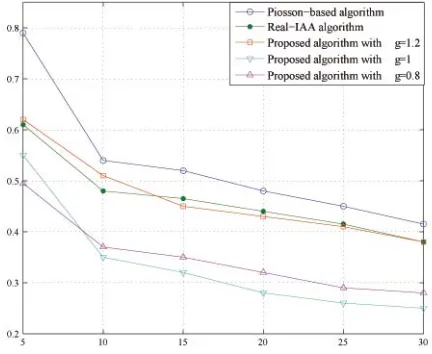
Figure 7 shows the relative error (ReError) performance of the algorithms with a single extended target in diﬀerent noise levels. The ReError is computed as

ReError = σ−σˆ2

σ₂ (19)

It can be seen in Figure 7 that the Poisson-based MAP algorithm has higher ReError under various SNR levels, while the proposed MAP algorithm is better than the conventional algorithms. The proposed algorithm has the similar ReError with Real-IAA algorithm in high SNR conditions whenγ = 1.2. It is superior to the Real-IAA algorithm with sparse constraint. The reason is that the proposed MAP algorithm provides reasonable prior information about the target distribution which leads to more stable solution to the forward-looking imaging problem.

5. CONCLUSION

In this paper, a Bayesian deconvolution method is proposed to overcome the low cross-range resolution problem of forward-looking area in motion platforms. The generalized Gaussian distribution is considered as the prior information of target scattering coefficient to realize high image quality and resolution because of the variability. We can control the statistic parameter of this distribution to make the proposed algorithm suitable for different applications. Simulation results verify the effectiveness of the proposed deconvolution algorithm.

REFERENCES

1. Schiavulli, D., F. Nunziata, G. Pugliano, and M. Migliaccio, “Reconstruction of the normalized radar cross section ﬁeld from gnss-r delay-doppler map,”IEEE Journal of Selected Topics in Applied Earth Observations and Remote Sensing, Vol. 7, No. 5, 1573–1583, 2014.

2. Ausherman, D. A., A. Kozma, J. L. Walker, H. M. Jones, and E. C. Poggio, “Developments in radar imaging,”IEEE Transactions on Aerospace and Electronic Systems, Vol. 4, No. AES-20, 363–400, 1984.

3. Curlander, J. C. and R. N. McDonough, Synthetic Aperture Radar, John Wiley & Sons, 1991. 4. Jakowatz, C. V., D. E. Wahl, P. H. Eichel, D. C. Ghiglia, and P. A. Thompson, Spotlight-mode

Synthetic Aperture Radar: A Signal Processing Approach, Springer Science & Business Media, 2012.

5. Loehner, A., “Improved azimuthal resolution of forward looking sar by sophisticated antenna illumination function design,” IEE Proceedings — Radar, Sonar and Navigation, Vol. 145, No. 2, 128–134, 1998.

6. Dai, S. and W. Wiesbeck, “High resolution imaging for forward looking sar with multiple receiving antennas,” IEEE 2000 International Geoscience and Remote Sensing Symposium, 2000. Proceedings. IGARSS 2000, Vol. 5, 2254–2256, IEEE, 2000.

7. Espeter, T., I. Walterscheid, J. Klare, A. R. Brenner, and J. H. Ender, “Bistatic forward-looking sar: results of a spaceborne-airborne experiment,” IEEE Geoscience and Remote Sensing Letters, Vol. 8, No. 4, 765–768, 2011.

8. Wu, J., Z. Li, Y. Huang, J. Yang, H. Yang, and Q. H. Liu, “Focusing bistatic forward-looking sar with stationary transmitter based on keystone transform and nonlinear chirp scaling,” IEEE Geoscience and Remote Sensing Letters, Vol. 11, No. 1, 148–152, 2014.

9. H¨ogbom, J., “Aperture synthesis with a non-regular distribution of interferometer baselines,”

Astronomy and Astrophysics Supplement Series, Vol. 15, 417, 1974.

(10)

10 Zhang et al.

11. Bose, R., A. Freedman, and B. D. Steinberg, “Sequence clean: A modiﬁed deconvolution technique for microwave images of contiguous targets,” IEEE Transactions on Aerospace and Electronic Systems, Vol. 38, No. 1, 89–97, 2002.

12. Bayliss, E. T., “Design of monopulse antenna diﬀerence patterns with low sidelobes,”Bell System Technical Journal, Vol. 47, No. 5, 623–650, 1968.

13. Sherman, S. M. and D. K. Barton,Monopulse Principles and Techniques, Artech House, 2011. 14. Caorsi, S., A. Massa, M. Pastorino, and A. Randazzo, “Optimization of the diﬀerence patterns

for monopulse antennas by a hybrid real/integer-coded diﬀerential evolution method,” IEEE Transactions on Antennas and Propagation, Vol. 53, No. 1, 372–376, 2005.

15. P´erez-Mart´ınez, F., J. Garcia-Fominaya, and J. Calvo-Gallego, “A shift-and-convolution technique for high-resolution radar images,”IEEE Sensors Journal, Vol. 5, No. 5, 1090–1098, 2005.

16. Munoz-Ferreras, J., J. Calvo-Gallego, F. P´erez-Mart´ınez, A. Blanco-del Campo, A. Asensio-Lopez, and B. Dorta-Naranjo, “Motion compensation for isar based on the shift-and-convolution algorithm,” 2006 IEEE Conference on Radar, 5, IEEE, 2006.

17. Ly, C., H. Dropkin, and A. Z. Manitius, “Extension of the music algorithm to millimeter-wave (mmw) real-beam radar scanning antennas,” AeroSense 2002, 96–107, International Society for Optics and Photonics, 2002.

18. Uttam, S. and N. A. Goodman, “Superresolution of coherent sources in real-beam data,” IEEE Transactions on Aerospace and Electronic Systems, Vol. 46, No. 3, 1557–1566, 2010.

19. Zhang, Y., Y. Zhang, Y. Huang, J. Yang, Y. Zha, J. Wu, and H. Yang, “Ml iterative superresolution approach for real-beam radar,”2014 IEEE Radar Conference, 1192–1196, IEEE, 2014.

20. Zhang, Y., Y. Zhang, W. Li, Y. Huang, and J. Yang, “Angular superresolution for real beam radar with iterative adaptive approach,”2013 IEEE International Geoscience and Remote Sensing

Symposium (IGARSS), 3100–3103, IEEE, 2013.

21. Zhang, Y., W. Li, Y. Zhang, Y. Huang, and J. Yang, “A fast iterative adaptive approach for scanning radar angular superresolution,” IEEE Journal of Selected Topics in Applied Earth Observations and Remote Sensing, Vol. PP, No. 99, 1–10, 2015.

22. Tan, X., W. Roberts, J. Li, and P. Stoica, “Sparse learning via iterative minimization with application to mimo radar imaging,” IEEE Transactions on Signal Processing, Vol. 59, No. 3, 1088–1101, 2011.

23. Xu, G., M. Xing, L. Zhang, Y. Liu, and Y. Li, “Bayesian inverse synthetic aperture radar imaging,”

IEEE Geoscience and Remote Sensing Letters, Vol. 8, No. 6, 1150–1154, 2011.

24. Guan, J., J. Yang, Y. Huang, and W. Li, “Maximum a posteriori based angular superresolution for scanning radar imaging,”IEEE Transactions on Aerospace and Electronic Systems, Vol. 50, No. 3, 2389–2398, 2014.

25. Zha, Y., Y. Huang, Z. Sun, Y. Wang, and J. Yang, “Bayesian deconvolution for angular super-resolution in forward-looking scanning radar,” Sensors, Vol. 15, No. 3, 6924–6946, 2015.

26. Osher, S., M. Burger, D. Goldfarb, J. Xu, and W. Yin, “An iterative regularization method for total variation-based image restoration,”Multiscale Modeling&Simulation, Vol. 4, No. 2, 460–489, 2005.

27. Golub, G. H., P. C. Hansen, and D. P. O’Leary, “Tikhonov regularization and total least squares,”

SIAM Journal on Matrix Analysis and Applications, Vol. 21, No. 1, 185–194, 1999.

28. Vauhkonen, M., D. Vadasz, P. A. Karjalainen, E. Somersalo, and J. P. Kaipio, “Tikhonov regularization and prior information in electrical impedance tomography,” IEEE Transactions on Medical Imaging, Vol. 17, No. 2, 285–293, 1998.