CRACK DETECTION USING A HYBRID FINITE
DIF-FERENCE FREQUENCY DOMAIN AND PARTICLE
SWARM OPTIMIZATION TECHNIQUES
S. H. Zainud-Deen, W. M. Hassen, and K. H. Awadalla
Faculty of Electronic Engineering Menoufia University
Menouf, Egypt
Abstract—A hybrid technique based on finite-difference frequency domain (FDFD) and particle swarm optimization (PSO) techniques is proposed to reconstruct the angular crack width and its position in the conductor and ability to detect the crack width, position, and its depth in single and multilayer dielectric objects. FDFD is formulated to calculate the scattered field after illuminating the object by a microwave transmitter. Two-dimensional model for the object is used. Computer simulations have been performed by means of a numerical program; results show the capabilities of the proposed approach. This paper presents a computational approach to the two dimensional inverse scattering problem based on FDFD method and PSO technique to determine the crack position, width and depth. By using the scattered field, the specifications of the crack are reconstructed.
1. INTRODUCTION
Crack detection is one of the important tasks for the industrial materials and products, since even small crack on the product surface could be fatal from the standpoint of safety. Traditionally, acoustic or electromagnetic waves have been used to detect the crack non-destructively. The crack width and length may be inspected by scanning the actual surface picture. But the depth of small crack may be difficult to evaluate nondestructively. A simple estimation formula for a crack depth on a conducting ground plane using the radar cross section dip is explained in [1].
The objective of the inverse scattering is to determine the electromagnetic properties of the scatterer from scattered field measured outside. Inverse scattering problems have attracted attention in the past few years [2–4]. The detection of the crack represents a complex inverse scattering problem that needs to be solved iteratively. That means the error between the measured data and the scattered fields computed from the trial solution is minimized at the end of the iteration, and the trial solution is then progressively adjusted towards the width, position, and depth of the crack. It is well-known that traditional deterministic techniques [5, 6] used for fast reconstruction of microwave images suffer from a major drawback, where the final image is highly dependent on the initial trial solution. In addition, it is often difficult to decide the adequacy of the initial trial solution for ensuring the correctness of the final solution. To overcome this obstacle, population based stochastic methods such as the genetic algorithm (GA) and PSO have become attractive alternatives to reconstruct microwave images [7, 8]. These techniques consider the imaging problem as a global optimization problem by imparting each individual within the population with its own fitness value as per the objective function defined for the problem, and reconstruct the correct image by searching for the optimal solution through the use of either rivalry or cooperation strategies in the problem space.
In this paper, the FDFD is used for the direct problem, a hybrid technique from FDFD and PSO is used for the inverse electromagnetic scattering problem. For the direct problem, the scattered field is to be calculated using the FDFD method assuming that the crack position, width and depth are known. For the inverse problem, the crack position, width, and depth are determined where the scattered field in free space is given using the global searching scheme PSO. This paper is organized as follows. In Section 2, the theoretical formulation for the FDFD method is presented. The general principle of the PSO is described. Numerical results for various cracks in conducting and dielectric objects in two dimensions are given in Section 3. Section 4 is the conclusions.
2. THEORETICAL BACKGROUND
2.1. FDFD Method
Starting from Maxwell’s equations for the total electric and magnetic fields for time harmonic convention ejωt, and σ= 0
∇ ×E¯
total =−jωμH¯total
∇ ×H¯total =jωεE¯total
By separating the total fields into incident and scattered field components, then
∇ ×E¯inc+ ¯Escat=−jωμH¯inc+ ¯Hscat ∇ ×H¯
inc+ ¯Hscat
=jωεE¯inc+ ¯Escat
(2)
The FDFD method is based on approximating the spatial derivative by finite differences. The first step in constructing an FDFD algorithm is to discretize the computational domain into a number of cells. Yee [9], constructed an algorithm that solves for both electric and magnetic fields using Maxwell’s equations. Based on the Yee space lattice, one can fit these field components to the FDFD expressions when the second-order accurate central difference scheme is used to discretize the space derivatives in Maxwell’s equations. To truncate the computational domain, layers of absorbing boundary based on the perfectly matched layer (PML) technique are used. The finite difference frequency domain is simplest in formulation and most flexible in modeling arbitrarily shaped inhomogenously filled and anisotropic scatterers. A detailed discussion of the FDFD method is provided in [10, 11].
2.2. The Procedure
In this work, the FDFD method, for the first time, has been used to get the scattered field for a certain known crack (position, width, and depth) as the first step. The crack used is specified and assumed to satisfy what might actually exist in real life. The second step is to assume several initial cracks, which are completely different from one used in the first step. Then, using the FDFD to get the scattered field from each crack. The third step is to find out the mean square error for each of the cracks of the second step with the results of the first step to be considered as the measured results. The fourth and final step is to apply the PSO algorithm on the population generated in the second and third steps to go iteratively to the optimum solution, which should be within a certain specified value of the error between the scattered field of Step 1 and the scattered field of the final achieved estimation of the crack.
2.3. PSO Algorithm
fitness. The previous best value is called “personal best”,Pbest. It also
has another value called “global best”,Gbest, which is the best value of
all the particlesPbest in the swarm for each iteration. The basic concept
of PSO technique lies in accelerating each particle towards itsPbest and
theGbest locations at each time step. The velocity and position of the
particles are changed according to Equations (3) and (4) respectively. Vid andXidrepresent the velocity and position of theith particle with
“d” dimensions respectively.
Vid = W ×Vid+C1×rand1×(Pbestid−Xid)
+C2×rand2×(Gbestid−Xid) (3)
Xid = Xid+Vid (4)
where W is the inertia weight that controls the exploration and exploitation of the search space. The random number functionrand1
and rand2 returns a number between 0.0 and 1.0. C1 and C2,
the cognition and social components respectively are the acceleration constants which change the velocity of a particle towards thePbestand
Gbest. A detailed discussion of the particle swarm optimizer used in
this paper is provided in [12, 13].
By starting from a defined residual as the difference between the calculated scattered field, Escat and the measured scattered field, Emeas, as
Ediff = Escat −Emeas (5)
The optimization will then be performed on the square normF F =Escat −Emeas2 (6) The goal is then to find the global minimum of this function.
3. NUMERICAL RESULTS
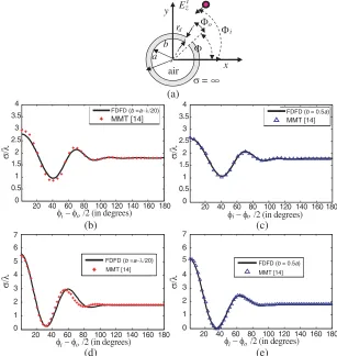
A computer program was written in Matlab code for implementing the FDFD formulation. This implementation was validated by computing the scattered field from several configurations includes slotted metallic and dielectric bodies. Fig. 1 shows the numerical results of the monostatic radar cross section of circular cylinder with a slot compared with the mode-matching technique (MMT) results [14] at frequency 300 MHz. The outer radius ofka= 3.456 and two different inner radii of b = a−λ/20 and b = 0.5a for Φo = 30◦ and Φo = 60◦. Excellent agreements are obtained.
crack in the object. Due to the absence of the measured data, the FDFD technique is used to synthesize the measured scattered field values for the computation of direct solution. Assume that a TMz (transverse magnetic to z-axis) plane wave is perpendicularly
incident upon a perfect conducting circular cylinder Einc = ˆ
azexp(jβ(xcos Φi+ysin Φi)). Φ, Φo,rd, and Φiare the crack position,
width, depth, and incident angle with respect to thex-axis, respectively (see Fig. 1(a)). A hybrid FDFD/PSO is used for reconstructing the crack position, width, and depth of the crack on the object.
i z (a) x y a b air 0 0.5 1 1.5 2 2.5 3 3.5 4
FDFD (b = a-ν/20) MMT [ 14 ]
20 40 60 80 100 120 140 160 180
FDFD (b=0.5 a) MMT [ 14 ]
0 1 2 3 4 5 6 7
FDFD (b=a-ν/20) T [ 14 ]
0 1 2 3 4 5 6 7
FDFD (b=0.5 a) MMT [ 14 ]
(b) (c) (d) (e) E Φi Φo rd σ = Ğ Φ
FDFD (b =a−λ/20)
MMT [14] σ/λ σ/λ 0 0.5 1 1.5 2 2.5 3 3.5 4
FDFD (b= 0.5a) MMT [14]
20 40 60 80 100 120 140 160 180
φ − φ /i o 2 (in degrees) φ − φ /i o 2 (in degrees)
FDFD (b =a−λ/20) MMT [14]
FDFD (b = 0.5a) MMT [14]
σ/λ σ/λ
20 40 60 80 100 120 140 160 180
φ − φ /i o 2 (in degrees)
20 40 60 80 100 120 140 160 180
φ − φ /i o 2 (in degrees)
y o y
o
x x
(a) (b)
air
(c) (d)
air
a b
air
x y
x
o
air
o
Φ = 61 Φ = 119
rd Φ
σ = Ğ σ = Ğ
rd
Φ i
z
E
Φ = 219 y Φ = 309
Φ Φ
rd
σ = Ğ σ = Ğ rd
i z
E
air
Figure 2. The position of the crack on circular cylinder ka = 3.456 and b = 0.5a at different values of crack position Φ, width Φo = 1◦, depthrd= 0.5a, and Φi = 0◦.
20 40 60 80 100 120 140 160 180 0
1 2 3 4 5 6
x y
a b
σ/λ
φ (in degrees)
Φ
i z E
air
σ = Ğ
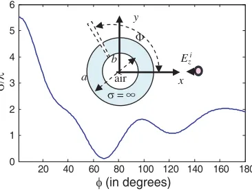
Figure 3. Bistatic RCS of circular cylinder with a crack position Φ = 119◦, width Φo = 1◦, and rd = 0.5a. The outer radius of
ka= 3.456 and inner radiusb= 0.5a.
Table 1. A comparison between the true and calculated values of position and width of the crack, the crack depthrd= 0.5a.
Position Φ Width Φo
(degree) (degree)
True Calculated True Calculated
61 61.001 1 0.9983
61 61.323 2 1.989
61 60.841 3 3.3853
119 119 1 1
119 118.86 2 2.1384
119 118.89 3 3
219 219.02 1 1.078
219 219.08 2 2.0674
219 219.14 3 3.4428
309 308.998 1 0.972
309 309.47 2 1.8828
309 309.29 3 3.0204
(a)
x y
air
a b
(b)
x y
air
b a
(c)
x y
air
b a r d= 0.05λ
rd rd
r d= 0.04λ
r d= 0.02λ
εr = 4 εr = 4
i z
E
Φ Φ
εr = 4
rd Φ
Table 2. A comparisons between the true and calculated values of position, width, and depth of the crack.
Position Φ Width Φo Depthrd
(degree) (degree)
True Calculated True Calculated True Calculated
61 61.028 1 1.22 0.05 0.05
(0.17a)
61 60.913 2 2 0.05 0.05
61 60.991 3 3 0.05 0.05
61 61.22 1 1.033 0.04 0.04086
(0.13a)
61 61.012 2 2.1243 0.04 0.03689
61 61.049 3 3 0.04 0.03993
61 61.201 1 1.00121 0.02 0.023242
(0.07a)
61 61.101 2 2.0932 0.02 0.0245
61 60.8789 3 2.887 0.02 0.02
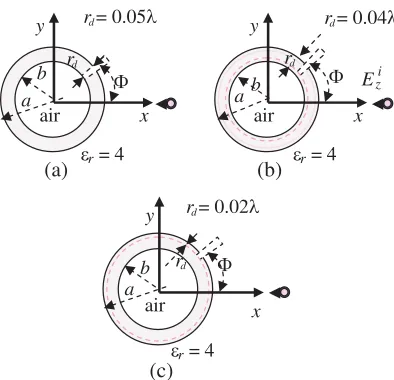
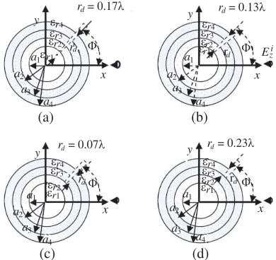
Figure 4 shows the reconstruction of the crack position Φ, width Φo, and depth rd of circular cylindrical dielectric tube with outer
radius “a” = 0.3λand inner radius “b” = 0.25λ and relative dielectric constantεr= 4. Table 2 shows a comparison between the true and the
calculated values using PSO technique. Good agreement is obtained.
FDFD
i z
E y
εr4
εr3
εr2
εr1 x
a1
a2
a3
a4
0 1 2 3 4 5 6 7 8 9
20 40 60 80 100 120 140 160 180
φ (in degrees)
σ/λ
Hybrid Method [15]
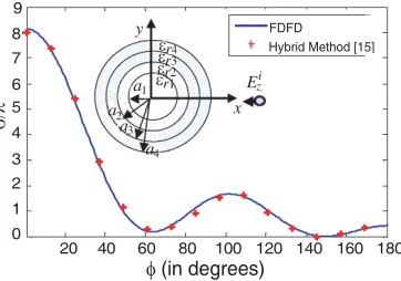
Figure 5. Bistatic radar cross section pattern of four layered dielectric object Φi = 0◦, (a1 = 0.15λ, a2 = 0.2λ, a3 = 0.25λ, a4 = 0.3λ), and
Figure 5 compares the bistatic radar cross section patteren of a four layered dielectric object using the FDFD and that obtained by Jankovic et al. [15]. The object dimensions area1 = 0.15λ,a2 = 0.2λ,
a3 = 0.25λ, a4 = 0.3λ, εr1 = 8, εr2 = 6, εr3 = 4, and εr4 = 2
for TMz plane wave. Good agreement is depicted. Fig. 6 shows the
reconstruction of the crack width Φo and depthrdon the object, crack
position Φ = 61◦. Table 3 shows a comparison between the true and the
r = 0.17d λ r = 0.13d λ
y εr4 y
εr3
εr2
εr1
a1 a2 a3 a4 x x i z E a1 a2 a3 a4
εr4
εr3
εr2
εr1
rd r
d
Φ Φ
(a) (b)
r = 0.07d λ r = 0.23d λ
y y
εr4
εr3
εr2
εr1
a1 a2
a3 a4
x rdΦ
x rdΦ a1
a2
a3 a4
εr4
εr3
εr2
εr1
(c) (d)
Figure 6. The reconstruction of the crack depth on four layered dielectric object. (a1 = 0.15λ, a2 = 0.2λ, a3 = 0.25λ, a4 = 0.3λ)
and (εr1 = 8, εr2 = 6, εr3 = 4, εr4 = 2) at crack position Φ = 61◦,
Φo= 1◦ and Φi= 0.
x y
air
a b
εr = 4
rd
rd i
z
E Φ
Φ1 2
Figure 7. Bistatic pattern of circular cylindrical dielectric tube with two crack positions Φ1 and Φ2. The outer radius a= 0.3, b = 0.25λ,
calculated values using PSO technique. Good agreement is obtained. Fig. 7 shows the reconstruction of the circular cylindrical dielectric tube with inner radius b= 0.25λ and outer radiusa= 0.3λ with two crack positions Φ1 and Φ2. Table 4 shows a comparison between the
true and the calculated values using PSO technique. Good agreement is obtained. To improve the accuracy, more iterations will be needed.
Table 3. A comparisons between the true and calculated values of width, and depth of the crack.
Width Φo Depthrd
(degree)
True Calculated True Calculated
1 0.9967 0.03 (0.1a4) 0.02986
1 1.0014 0.07 (0.23a4) 0.069864
1 1 0.13 (0.43a4) 0.130401
1 1 0.17 (0.57a4) 0.168915
2 2.0083 0.03 (0.1a4) 0.031995
2 2.0118 0.07 (0.23a4) 0.070409
2 1.98559 0.13 (0.43a4) 0.13167
2 1.97928 0.17 (0.57a4) 0.16883
3 3 0.03 (0.1a4) 0.03039
3 3 0.07 (0.23a4) 0.07276
3 3 0.13 (0.43a4) 0.13183
3 3 0.17 (0.57a4) 0.17
Table 4. A comparisons between the true and calculated values of width, and depth of the crack.
Position Φ1, Φ2 Width Φo1, Φo2
(degree) (degree)
True Calculated True Calculated
4. CONCLUSION
The hybrid technique, FDFD/PSO for reconstruction of the crack position, and depth has been proposed. The forward problem is solved using the FDFD method. The inverse problem is reformulated into an optimization one and then the global searching scheme PSO is employed to search the parameter space. By using the PSO, the crack position, width and depth can be successfully reconstructed. Numerical results have been carried out and good reconstruction for crack has been obtained even in multilayer dielectric object or multiple cracks on the object.
REFERENCES
1. Sekiguchi, H. and H. Shirai, “A simple estimation formula for a crack depth using the RCS dip,” Proc. IEEE AP-S Int. Conf., Vol. 3, 220–223, Columbus, OH, USA, Jun. 2003.
2. Qing, A., C. K. Lee, and L. Jen, “Electromagnetic inverse scattering of two-dimensional perfectly conducting objects by real-coded genetic alogrithm,” IEEE Trans. Geoscience and Remote Sensing, Vol. 39, No. 3, 665–676, Mar. 2001.
3. Zainud-Deen, S. H., M. S. Ibrahim, and E. M. Ali, “A hybrid finite difference frequency domain and particle swarm optimization techniques for forward and inverse electromagnetic scattering problems,” The 23rd Annual Review of Progress in Applied Computational Electromagnetics, 1575–1580, Verona, Italy, Mar. 2007.
4. Zainud-Deen, S. H., W. M. Hassen, E. M. Ali, K. H. Awadalla, and H. A. Sharshar, “Breast cancer detection using a finite difference frequency domain and particle swarm optimization techniques,” Progress In Electromagnetics Research B, Vol. 3, 35–46, 2008. 5. Souvorov, A. E., A. E. Bulyshev, S. Y. Semenov, R. H. Svenson,
A. G. Nazarov, Y. E. Sizov, and G. P. Tatsis, “Microwave tomography: A two-dimensional Newton iterative scheme,”IEEE Trans. Microw. Theory Tech., Vol. 46, 1654–1659, Nov. 1998. 6. Chew, W. C. and Y. M. Wang, “Reconstruction of
two-dimensional permittivity distribution using the distorted born iterative method,” IEEE Trans. Med. Imag., Vol. 9, 218–225, Jun. 1990.
optimization technique,” IEEE Trans. Microw. Theory Tech., Vol. 52, 1909–1916, 2004.
8. Xiao, F. and H. Yabe, “Microwave imaging of perfect conducting cylinders from real data by micro genetic algorithm coupled with deterministic method,”IEICE Trans. Electron., Vol. E81-C, 1784– 1792, 1998.
9. Yee, K. S., “Numerical solution of initial boundary value problems using Maxwell’s equations in isotropic media,” IEEE Trans. Antennas Propag., Vol. 14, No. 5, 302–307, May 1966. 10. Al Sharkawy, M. H., V. Demir, and A. Z. Elsherbeni, “Plane
wave scattering from three dimensional multiple objects using the iterative multiregion technique based on the FDFD method,”
IEEE Trans. Antennas Propag., Vol. 54, No. 2, 666–673,
Feb. 2006.
11. Zainud-Deen, S. H., E. El-Deen, and M. S. Ibrahem, “Electro-magnetic scattering by conducting/dielectric objects,” The 23rd Annual Review of Progress in Applied Computational Electromag-netics, 1866–1871, Verona, Italy, Mar. 2007.
12. Robinson, J. and Y. Rahmat-Samii, “Particle swarm optimization in electromagnetics,” IEEE Trans. Antennas Propag., Vol. 52, No. 2, 397–407, Feb. 2004.
13. Jin, N. and Y. Rahmat-Samii, “Advances in particle swarm optimization for antenna designs: Real-number, binary, signal-objective and multisignal-objective implementations,”IEEE Trans. An-tennas Propag., Vol. 55, No. 3, 556–567, Mar. 2007.
14. Noh, Y. C. and S. D. Choi, “TM scattering from hollow slotted circular cylinder with thickness,”IEEE Trans. Antennas Propag., Vol. 45, No. 5, 909–910, May 1997.