Scholarship@Western
Scholarship@Western
Electronic Thesis and Dissertation Repository
12-15-2017 10:00 AM
Assessment of Dynamic Effect of Transmission Line Conductor
Assessment of Dynamic Effect of Transmission Line Conductor
Longitudinal Reaction Due to Downburst Loading
Longitudinal Reaction Due to Downburst Loading
Ibrahim Ibrahim
The University of Western Ontario
Supervisor
El Damatty, Ashraf A.
The University of Western Ontario
Graduate Program in Civil and Environmental Engineering
A thesis submitted in partial fulfillment of the requirements for the degree in Master of Engineering Science
© Ibrahim Ibrahim 2017
Follow this and additional works at: https://ir.lib.uwo.ca/etd
Part of the Aerodynamics and Fluid Mechanics Commons, and the Structural Engineering Commons
Recommended Citation Recommended Citation
Ibrahim, Ibrahim, "Assessment of Dynamic Effect of Transmission Line Conductor Longitudinal Reaction Due to Downburst Loading" (2017). Electronic Thesis and Dissertation Repository. 5102.
https://ir.lib.uwo.ca/etd/5102
This Dissertation/Thesis is brought to you for free and open access by Scholarship@Western. It has been accepted for inclusion in Electronic Thesis and Dissertation Repository by an authorized administrator of
i
Due to the locality and non-stationary nature of downburst wind loading events, their effect on
the structural response of transmission line structures is of special nature that differs from
conventional atmospheric boundary layer wind loading. Acknowledging such difference, the
current thesis aims to quantify the dynamic effect associated with downburst loading on
transmission line systems. To achieve that, several steps had to be realized, including
experimentally verifying the numerical model used for analysis using wind field that was
generated using computational fluid dynamics. The verified model was extended from model
scale to full scale, where the wind field used for loading was a combination of mean component
generated using CFD, and turbulent component that was synthetically generated using a
statistically calibrated numerical technique. Results of the analyses showed that the
consideration of dynamic analysis did not affect the computed peak longitudinal reactions.
Finally, the wind field used was compared to field measurements to ensure the deduced
conclusions can be generalized.
Keywords
ii
Co-Authorship Statement
This thesis has been prepared in accordance with the regulations for an Integrated Article
format thesis stipulated by the School of Graduate and Postdoctoral Studies at Western
University. Statements of the co-authorship of individual chapters are as follows
Chapter 2: Numerical Simulation of WindEEE Dome Downburst Using Physical Roughness Elements
Numerical simulations and analyses were conducted by I. Ibrahim under close supervision of
Dr. A. A. El Damatty and Dr. H. Aboshosha with the co-operation of Dr. A. Elawady regarding
utilizing the experimental data.
Drafts of Chapter 2 were written by I. Ibrahim, and modifications were done under supervision
of Dr. A. A. El Damatty and Dr. H. Aboshosha. A paper co-authored by I. Ibrahim, H.
Aboshosha, A. A. El Damatty and A. Elawady will be submitted to the Journal of Wind and
Structures.
Chapter 3: The Effect of Downburst Wind Field Characteristics on the Longitudinal Forces on Transmission Towers
All the numerical models and analyses were conducted by I. Ibrahim under close supervision
of Dr. A. A. El Damatty. Drafts of Chapter 3 were written by I. Ibrahim and modifications
were done under supervision of Dr. A. A. El Damatty. A paper co-authored by I. Ibrahim and
A. A. El Damatty will be submitted to the Journal of Wind Engineering & Industrial
iii
Acknowledgments
With these few words, I would like to express my deep gratitude to those whom the past two
years would have never been as productive, enjoyable and bearable for the most part. Among
them, stands out my supervisor, Prof. Ashraf El Damatty, for the guidance he never failed to
be generous with, the encouragement I was usually seeking during the times I struggled with
my work, and being the role model he is for me and my fellow group members.
The help and valuable advice I received from Dr. Haitham Aboshosha are also acknowledged
with the sincerest gratefulness. The journey has had its crests and troughs, my colleagues in
the department have had a great role in helping me getting through. Some of them were really
supportive and always generous with their technical knowledge. Others were a necessity for
me to keep my temper and sometimes my sanity on the times the numerical models really got
on my nerves. The only person I could think of who belongs to both teams is Dr. Ahmed
Elshaer. I owe him a lot in return for his support, technical knowledge, and fun times we had
together.
Lastly, saving the my dearest words for my dearest people, I spend my days thanking God for
the family I have, doubting if anything I ever did or will ever do one day can prove me worthy
of the blessing I have, with that I mean my amazing parents. To them I owe everything I have
reached and everything I would ever reach. I am also grateful for the blessing of having my
amazing siblings; Aya, my twin sister whom I literally shared with every day of my life, Amr,
my younger, taller, cooler and funnier brother, my sister Zahraa, the light of our lives for the
past eight years, Khalid, my brother-in-law, the second redhead in our family, and lastly, the
iv
Table of Contents
Abstract ... i
Co-Authorship Statement... ii
Acknowledgments... iii
Table of Contents ... iv
List of Tables ... vi
List of Figures ... vii
Chapter 1 ... 1
1 Introduction ... 1
1.1 Background ... 1
1.2 Studies of Downburst Loading on Transmission Line Systems ... 4
1.3 Structural Analysis of Transmission Lines ... 7
1.4 Downburst Wind Field ... 9
1.5 Objectives of the Study ... 10
1.6 Organization of Thesis ... 10
1.7 References ... 12
Chapter 2 ... 17
2 Numerical Simulation of WindEEE Dome Downburst Using Physical Roughness Elements ... 17
2.1 Introduction ... 17
2.2 Experimental Simulation ... 22
2.3 Numerical Model Setup ... 26
2.3.1 LES Governing Equations ... 26
2.3.2 Model Details ... 27
2.4 Results and Discussion ... 31
v
2.4.3 Mean Component of Wind Field ... 39
2.4.4 Turbulent Component of Wind Field ... 40
2.5 Conclusions ... 45
2.6 References ... 46
Chapter 3 ... 52
3 The Effect of Downburst Wind Field Characteristics on the Longitudinal Forces on Transmission Towers ... 52
3.1 Introduction ... 52
3.1.1 Background ... 52
3.1.2 Problem Definition... 55
3.2 Model-Scale Analysis ... 61
3.2.1 Numerical Model ... 61
3.2.2 Comparison of Numerical Results with Experimental Measurements ... 66
3.3 Full-Scale Analysis ... 68
3.3.1 Wind Field ... 68
3.3.2 Numerical Model ... 76
3.3.3 Results and Discussion ... 78
3.4 Further Considerations and Analysis ... 83
3.5 Conclusions ... 88
3.6 References ... 90
Chapter 4 ... 97
4 Conclusions and future work ... 97
4.1 Conclusions ... 97
4.2 Future work ... 100
vi
List of Tables
Table 3-1 Properties of the conductor system and the downburst ... 77
Table 3-2 Comparison of downburst characteristics from different studies ... 84
vii
List of Figures
Chapter 1: Introduction
Figure 1-1 Components of transmission line system
“http://electrical-power-system.blogspot.ca” ... 2
Figure 1-2 A series of transmission line towers “https://www.thenews.com.pk/” ... 3
Figure 1-3 Oblique load case illustration ... 6
Figure 1-4 Broken cross-arm due to downburst event “Aboshosha et al. (2016a)” ... 7
Chapter 2: Numerical Simulation of WindEEE Dome Downburst Using Physical Roughness Elements Figure 2- 1 Schematic view of the impinging jet model ... 20
Figure 2- 2 Schematic view of the WindEEE dome as per (Jubayer et al. 2016) ... 22
Figure 2- 3 Probe tower locations and probe heights in meters ... 23
Figure 2- 4 Radial velocity profiles comparison for (a) open and (b) suburban terrain ... 24
Figure 2- 5 Decomposed time history ... 25
Figure 2- 6 Boundary conditions assignment for different boundaries with details of inlet .. 28
Figure 2- 7 Influence Zone ... 29
Figure 2- 8 Grid dependency plot ... 30
Figure 2- 9 Experimental smoke visualization vs CFD velocity contour ... 31
Figure 2- 10 Development of wind field represented by velocity contours for different τ = t / Tmax at P1 ... 34
viii
Figure 2- 13 Effect of averaging period on mean of fluctuating residuals ... 37
Figure 2- 14 Decomposed time history at R/Dj = 1 and Z/Dj = 0.078 ... 38
Figure 2- 15 Mean radial velocity validation ... 39
Figure 2- 16 Power spectral density function validation ... 40
Figure 2- 17 Effect of LES grid size on captured frequencies (-) EXP (….) CFD ... 41
Figure 2- 18 Turbulence intensity profile for different inlet turbulence ratios ... 42
Figure 2- 19 Turbulence intensity vs mean velocity envelope distribution along height for different radial distances for Suburban Terrain ... 44
Figure 2- 20 Turbulence intensity vs mean velocity envelope distribution along height for different radial distances for Open Terrain ... 44
Chapter 3: The Effect of Downburst Wind Field Characteristics on the Longitudinal Forces on Transmission Towers Figure 3- 1 Oblique load case illustration ... 56
Figure 3- 2 Flow chart of the work conducted ... 59
Figure 3- 3 Mean radial velocity vs Time for downburst wind field at a probe point ... 62
Figure 3- 4 Layout of tested conductor system ... 63
Figure 3- 5 Leaf spring instrumentation at cable ends ... 63
Figure 3- 6 Time history of radial velocity for a probe point ... 64
ix
numerical model... 66
Figure 3- 9 Comparison between fluctuating component of longitudinal reaction for (a)
experimental and (b) SAP 2000 analysis ... 67
Figure 3- 10 Flow chart of turbulence generation technique ... 72
Figure 3- 11 Generated turbulence for a sample point ... 74
Figure 3- 12 Comparison between target and generated coherencies for (a) radial and (b)
circumferential directions ... 75
Figure 3- 13 Time history of radial velocity after superimposing generated turbulence ... 76
Figure 3- 14 Schematic of analyzed structure system ... 77
Figure 3- 15 Time history of longitudinal reaction for quasi-static analysis compared to
dynamic analysis ... 78
Figure 3- 16 Time history of longitudinal reaction for turbulent wind field compared to fully
correlated wind field ... 79
Figure 3- 17 Normalized cumulative PSDF for (a) Full time history (b) peak zone ... 81
Figure 3- 18 Illustration of the annotations used to characterize the downburst time history 83
Figure 3- 19 Modified time histories of radial velocity ... 85
Figure 3- 20 Mode frequencies compared to shedding frequency for (a) model scale and (b)
unmodified full scale... 86
x
Chapter 1
1
Introduction
1.1
Background
Throughout the past century, electricity has been a major component of and contributor to
how our modern world has evolved to be. Furthermore, the role of electricity in our lives
has only intensified and gained more importance as new technologies are totally dependent
on the undisturbed availability of energy provided by electricity. Such reliability projects
great importance on the sustainability of electricity transmission line systems as a key
component of a functioning electric network. As shown in Figure 1-1, transmission line
systems consist of different components. These can be mainly classified in the order of
load transfer from a structural perspective as follows; conductors and wires transfer the
loads across spans axially to the insulators that in this case act as the supports for these
non-linear components. The insulators then convey the load axially again to the nearest
tower components, the cross arms, which is where the insulators are attached. The loads
are then transferred through the tower members, that in turn act as a truss that can resist
forces and moments developed, and finally convey these forces to the supporting
foundation structure. Within the given sequence, structural engineers must ensure that
Accordingly, structural engineers must be aware of the types of loads transmission
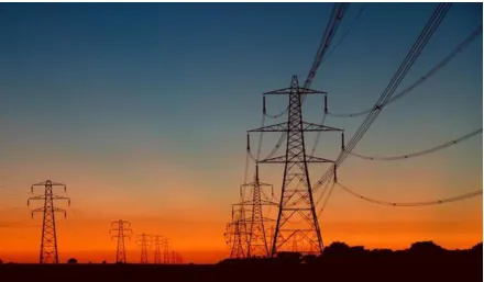
structures are susceptible to. As seen in Figure 1-2, transmission line structures usually
extend through great distances in relatively open exposures, making them fully exposed to
weather related loading events. Judging by how current design guide lines, such as
ASCE-74 (2010), are structured, it is widely recognized that weather related loading is the
governing type of loading when designing transmission line systems. Yet, some weather
loading phenomena, such as tornadoes and downbursts, are still far from being completely
incorporated in the design of sustainable transmission line systems. This is mainly due to
two things; first, the complexity of these events, which makes them hard to implement as
loading phenomena, unlike straight wind, which is arguably fully comprehended, and thus
its current incorporation can be considered as a trusted representation of the loads
associated with the phenomenon. The second thing, which relates more to downbursts, is
the absence of sufficient database of event occurrence, which in turn complicates the efforts
to quantify the precise impact these events have on transmission line systems. Figure 1-1 Components of transmission line system
Focusing on the downburst phenomenon, it was first defined by the prominent
meteorologist Ted Fujita, who defined downbursts as a descending column of air that
impinges the ground, and causes a radial outburst resulting in devastating wind speeds
(Fujita 1985). Such event is characterized by being a localized non-stationary event. The
locality is due to the comparability of the phenomenon scale compared to the dimensions
of the transmission line structures. While the descending column of air can be between
1500 to 3000 meters in diameter (Hjelmfelt 1988), the span of transmission line is in the
order of hundreds of meters. This comparability in scale dictates a difference in the
consideration of downburst loading on transmission line structures compared to normal
wind loading where consequent spans are assumed to experience the same loading. In
addition, the resulting wind field is described as being non-stationary as it demonstrates a
structure system, as well as combine with the locality of phenomenon to introduce new
loading conditions on spans of the transmission line systems. These new loading
circumstances demonstrated a devastating effect on transmission line systems, where
failures reported worldwide were linked to downburst events (Kanak et al. 2007, Li 2000,
McCarthy and Melsness 1996, Zhang 2006). These failures have motivated researchers to
study the effect of downburst loading on transmission line systems as discussed in the next
section.
1.2
Studies of Downburst Loading on Transmission Line
Systems
As a result of the devastating events mentioned in the previous section, a wide spectrum of
researchers have been studying the effect of downburst loading on transmission line
systems and efforts to mitigate such hazards to ensure transmission line structures can
sustainably withstand such loads. Researchers differed in terms of the considered structure
system under downburst loading; researchers like Aboshosha et al. (2016), Lin et al.
(2012), Shehata et al. (2005), Shehata and El Damatty (2007) and Darwish and El Damatty
(2011)considered the tower-line system with both the towers and the conductors included
in the analyses to study their combined behavior under down burst loading. Other
researchers like Mara et al. (2010), Mara and Hong (2013) and Savory et al. (2001) only
considered the supporting structures, focusing on the responses of the towers due to the
downburst wind field. This was counter-acted by other researches who considered the
downburst wind field to be more important in the case of conductor systems due to the
locality of the loading phenomenon, and its comparable scale to the spans of the conductor
El Damatty (2015), (2014a), (2014b), Darwish et al. (2010) and Elawady and El Damatty
(2016). These researchers studied the behavior of conductor systems to downburst loading
under different loading configurations ignoring the effect the towers might impose on the
analysis due to their relative rigidity compared to the conducting lines. The outcome of
such research mainly focused on the effect the locality of the downburst had on the
computed responses of the conductor systems. One of which, Elawady and El Damatty
(2016), mainly studied the effect downbursts have on the computing of longitudinal
reactions of a conductor system. The study carried on from where researchers like Darwish
and El Damatty (2011) and Shehata and El Damatty (2007) have concluded. These
previous studies examined different loading cases associated with different spatial
configurations of downburst positioning relevant to the studied structure. One of the load
cases examined is the oblique load case. As shown in Figure 1-3, this is the case where the
line joining the downburst center is at an angle from the line perpendicular to the tower of
interest. This is configuration is expected to cause differential loading across consecutive
spans. This can be of specific importance for transmission structure elements like tower
cross-arms. The differential loading causes the development of a longitudinal reaction that
would be transferred from the conductors to the tower structure. While current design
guidelines do not take such case into consideration, certain cases with high velocities of
downburst events can be devastating to cross-arms as shown in Figure 1-4. Accordingly,
the study performed by Elawady and El Damatty (2016) considered the oblique load case
and its effect on the magnitude of the computed longitudinal reaction using the quasi-static
numerical technique developed by Aboshosha and El Damatty (2014b). The study
derive generic conclusions on the values longitudinal reactions. The outcome of this
research was compiled into a comprehensive set of charts that can be easily used by
practitioners to compute design values of longitudinal reactions based on the conductor’s
geometry and physical properties. However, such a robust technique relied on the
conclusions stated by previous researchers that downburst loading can sufficiently be
analyzed using quasi-static analysis (Darwish et al. 2010).
Yet, the fact the differential loading is the cause of the developed longitudinal reaction, can
add more weight to the dynamic analysis, which considers the spatial correlations between
distant nodes, a key parameter that is overlooked by quasi-static analysis. The next section
will discuss the previous efforts that led to the conclusion of the quasi-static analysis being
sufficient for such types of systems, and how this might be invalid for the case in hand. Transmission line
R 𝜃
Dj
1.3
Structural Analysis of Transmission Lines
Previous researchers who structurally analyzed the transmission line systems mostly used
the quasi-static analysis approach (Darwish and El Damatty 2011, Elawady and El Damatty
2016, Shehata et al. 2005 and Shehata and El Damatty 2007). Yet, other researchers
considered the dynamic effect the downburst loading might have on the responses of the
structure systems, specially conductor spans (Aboshosha and El Damatty 2015b, Darwish
et al. 2010 and Lin et al. 2012). For the researchers evaluating the dynamic effects
numerically, a major challenge was the choice of a representative aerodynamic damping
expression that addresses both the physical properties of the conductors, as well as the
transient nature of the downburst event. Accordingly, the expression given by Davenport
(1962) and shown in equation (1-1) has been considered to represent the effect of the
physical properties of the conductors on the value of aerodynamic damping, yet was
deemed unsuitable for the use in the analysis of downburst loading analysis as it does not
address the non-stationarity of the loading event.
𝜻𝒂𝒊= 𝝆𝑪𝑫𝑫𝑽 𝟒𝝅𝒎𝒇𝒊
(1-1)
Where 𝜻𝒂𝒊 is the aerodynamic damping value per mode 𝑖 , 𝝆 is the air density, 𝑪𝑫 is the drag
coefficient, 𝑫 is the conductor diameter, 𝑽 is the wind velocity, 𝒎 is the conductor mass, and
𝒇𝒊 is the mode’s frequency.
To address the transient nature of the loading, researchers like Darwish et al. (2010)
modified the above expression, by replacing the constant wind velocity term by another
term that varies with time. Such a modification can require special computational
measures, since the changing values of damping might not be accommodated by
mainstream structural analysis programs, which triggers the need of developing in-house
coding such as the models developed by Darwish et al. (2010) and Aboshosha et al.
(2016b). Nevertheless, these approaches lacked the creditability the original approach
(Davenport 1962) had through experimental validation of the proposed expression.
Accordingly, any further analysis done should make use of reliable experimental testing at
reasonable scales to make sure the derived conclusions can be used with confidence. Upon
deciding on a valid numerical approach to dynamically analyze the structure system, the
use of a validated wind field with nature-like turbulence is a major component that cannot
be spared. The next section will discuss the different options presented by previous
researchers to obtain downburst wind field with turbulent component suitable for dynamic
1.4
Downburst Wind Field
As mentioned in the first section of this chapter, downburst events are localized events,
which means that the event usually occurs at micro-scales, with an affected area only
several kilometers wide. Such localization has so far made it difficult for researchers to
capture downburst wind field data from field measurements. Instead, anemometer velocity
time histories provide a limited perspective on the downburst wind filed properties, with
no consideration of the spatial and temporal relations between distant points. Although this
is expected to change soon due to the advances in data capturing technologies and the new
Lidar systems capable of clearing out such ambiguities, the data available in the modern
literature still lacks a full comprehension of spatiotemporal relations between points at
different positions. Therefore, previous studies that were interested in the dynamic analysis
of transmission line structure systems relied on computational fluid dynamics (CFD) to
resolve the flow using either kinematic (impinging jet) scheme, or thermodynamic (cooling
source) scheme to resemble the flow characteristics of downburst events. As such, the
wind field provided by Kim and Hangan (2007) utilized the impinging jet scheme to
produce the desired flow field. Yet, the flow field provided could only resolve for mean
components of the flow due to the choice numerical scheme used in CFD analysis.
Researchers like Darwish et al. (2010) extracted the turbulence component of the field
measurements reported by Holmes et al. (2008), and super imposed it on the mean wind
field resulting from the CFD simulation. Others like Aboshosha et al. (2016b) synthetically
generated the turbulent component using the technique described by Chen and Letchford
(2004) and Chay et al. (2006). However, both techniques used to create a turbulent
relations between points at which the turbulent component is generated. The overlooking
of characteristics like correlations and length scales can be deterministic in the case of
studying dynamic effect of downburst loading on transmission line systems due to the
comparability in the scales of the event and the structure system. Accordingly, a more
robust technique is to be used if the same superposition technique is used to create a wind
field including the turbulent component of the flow.
1.5
Objectives of the Study
The current study investigates the validity of the assumptions presumed by Elawady and
El Damatty (2016) which will be discussed elaborately in chapter 3 of this thesis.
Accordingly, the objectives of the current study are as follows:
1. Assess the dynamic effect downburst loading might have on the computed
longitudinal reactions of conductor systems.
2. Quantify the effect of considering the correlations between spatially distinct points
on the values of longitudinal reactions.
3. Judge the applicability of the conducted analysis in regard to the used wind field
compared to field measured data.
1.6
Organization of Thesis
This thesis is organized following the “Integrated Article” format. The current chapter
introduces the studied topic, along with the key points targeted by the research as objectives
of the study. The following chapters address the objectives mentioned as follows:
Chapter 2: Numerical Simulation of WindEEE Dome Downburst Using Physical
This chapter aims to provide a detailed wind field of the downburst simulation conducted
in the WindEEE dome. Being the first of its kind, the WindEEE dome is able to produce
downbursts using the impinging jet model at wind tunnel testing scale. The study presented
in this chapter aims to replicate the experiment using Large Eddy Simulation (LES) CFD
model to capture the characterizing features of the wind field. The results captured from
the simulation were compared with the experiment for both the mean and the turbulent
components of the flow. The flow features were also examined at different positions in the
domain, and it was found that the geometry of the local components of the dome impose
an undesirable effect on the flow.
Chapter 3: The Effect of Downburst Wind Field Characteristics on the Longitudinal Forces
on Transmission Towers
In this chapter, the effect of downburst wind field characteristics, namely the turbulent
component and the characteristics of the mean component, are examined. Starting with the
turbulent component, the chapter first proposes a numerical model that is capable of
dynamically analyzing conductor systems under downburst loading. Utilizing the detailed
wind field availed by the study presented in chapter 2, the assumptions and hypothesis are
validated using an aero-elastic experiment that was conducted in the WindEEE dome. The
study was then extended to the full scale, studying the dynamic effect of downburst loading
on longitudinal reactions at tower structures. To do so, a synthetic turbulent component
was first generated and calibrated, then superimposed on previously available CFD mean
flow field. After deciding on the significance of the dynamic effect on the computed
reaction values, the following sections of the chapter compare the used wind field with data
CFD to available field measurements. Lastly, CFD wind fields were modified to match the
field measurements, and the effect of the applied modifications on the computed reactions
was reported.
Finally, the last chapter of this thesis presents the conclusions obtained from the performed
research, as well as recommendations for future work based on the results of this study.
1.7
References
Aboshosha, H., El Damatty, A., (2015a). Engineering method for estimating the
reactions of transmission line conductors under downburst winds. Eng. Struct. 99, 272–
284. doi:10.1016/j.engstruct.2015.04.010
Aboshosha, H., El Damatty, A.A., (2015b). Dynamic response of transmission line
conductors under downburst and synoptic winds. Wind Struct. An Int. J. 21, 241–272.
doi:10.12989/was.2015.21.2.241
Aboshosha, H., El Damatty, A.A., (2014a). Span Reduction Factor of Transmission
Line Conductors Under Downburst Winds Span Reduction Factor of Transmission Line.
J. Wind Eng. 11, 13–22. doi:10.3850/978-981-07-8012-8
Aboshosha, H., El Damatty, A.A., (2014b). Effective technique to analyze
transmission line conductors under high intensity winds. Wind Struct. An Int. J. 18, 235–
252. doi:10.12989/was.2014.18.3.235
Aboshosha, H., Elawady, A., El Ansary, A., El Damatty, A.A., (2016a). Review on
dynamic and quasi-static buffeting response of transmission lines under synoptic and
Aboshosha, H., Ibrahim, A., El Damatty, A.A., Hamada, A., (2016b). Dynamic
Behaviour of Transmission Lines Structures under Synoptic Wind Loads, in: 2016
CIGRE-IEC Colloquium.
ASCE-74, (2010). American Society of Civil Engineers (ASCE). Guidelines for
electrical transmission line structural loading. ASCE Manuals and Reports on Engineering
Practice, No. 74, New York (NY), USA; 2010.
Chay, M.T., Albermani, F., Wilson, R., (2006). Numerical and analytical simulation
of downburst wind loads. Eng. Struct. 28, 240–254. doi:10.1016/j.engstruct.2005.07.007
Chen, L., Letchford, C.W., (2004). A deterministic-stochastic hybrid model of
downbursts and its impact on a cantilevered structure. Eng. Struct. 26, 619–629.
doi:10.1016/j.engstruct.2003.12.009
Darwish, M.M., El Damatty, A.A., (2011). Behavior of self supported transmission
line towers under stationary downburst loading. Wind Struct. An Int. J. 14, 481–498.
doi:10.12989/was.2011.14.5.481
Darwish, M.M., El Damatty, A.A., Hangan, H., (2010). Dynamic characteristics of
transmission line conductors and behaviour under turbulent downburst loading. Wind
Struct. An Int. J. 13, 327–346. doi:10.12989/was.2010.13.4.327
Davenport, A.G., (1962). Buffeting of a suspension bridge by storm winds. J. ASCE
Elawady, A., El Damatty, A.A., (2016). Longitudinal force on transmission towers
due to non-symmetric downburst conductor loads. Eng. Struct. 127, 206–226.
doi:10.1016/j.engstruct.2016.08.030
Fujita, T.T., (1985). The downburst: microburst and macroburst. Satellite and
Mesometeorology Research Project (SMRP). Res. Pap. 210, Dep. Geophys. Sci. Univ.
Chicago.
Hjelmfelt, M.R., (1988). Structure and life cycle of microburst outflows observed in
Colorado. J. Appl. Meteorol. 900–927.
Holmes, J.D., Hangan, H.M., Schroeder, J.L., Letchford, C.W., Orwig, K.D.,
(2008). A forensic study of the Lubbock-Reese downdraft of 2002. Wind Struct. An Int. J.
11, 137–152. doi:10.12989/was.2008.11.2.137
Kanak, J., Benko, M., Simon, A., Sokol, A., (2007). Case study of the 9 May 2003
windstorm in southwestern Slovakia. Atmos. Res. 83, 162–175.
doi:10.1016/j.atmosres.2005.09.012
Kim, J., Hangan, H., (2007). Numerical simulations of impinging jets with
application to downbursts. J. Wind Eng. Ind. Aerodyn. 95, 279–298.
doi:10.1016/j.jweia.2006.07.002
Li, C.Q., (2000). A stochastic model of severe thunderstorms for transmission line
Lin, W.E., Savory, E., Mcintyre, R.P., Vandelaar, C.S., King, J.P.C., (2012). The
response of an overhead electrical power transmission line to two types of wind forcing. J.
Wind Eng. Ind. Aerodyn. 100, 58–69. doi:10.1016/j.jweia.2011.10.005
Mara, T.G., Galsworthy, J.K., Savory, E., (2010). Assessment of vertical wind loads
on lattice framework with application to thunderstorm winds. Wind Struct. An Int. J. 13,
413–431.
Mara, T.G., Hong, H.P., (2013). Effect of wind direction on the response and
capacity surface of a transmission tower. Eng. Struct. 57, 493–501.
doi:10.1016/j.engstruct.2013.10.004
McCarthy, P., Melsness, M., (1996). Severe weather elements associated with
September 5, 1996 hydro tower failures near Grosse.
Savory, E., Parke, G.A.R., Zeinoddini, M., Toy, N., Disney, P., (2001). Modelling
of tornado and microburst-induced wind loading and failure of a lattice transmission
tower. Eng. Struct. 23, 365–375. doi:10.1016/S0141-0296(00)00045-6
Shehata, A.Y., El Damatty, A.A., (2007). Behaviour of guyed transmission line
structures under downburst wind loading. Wind Struct. 10, 249–268.
Shehata, A.Y., El Damatty, A.A., Savory, E., (2005). Finite element modeling of
transmission line under downburst wind loading. Finite Elem. Anal. Des. 42, 71–89.
Zhang, Y., (2006). Status quo of wind hazard prevention for transmission lines and
Chapter 2
2
Numerical Simulation of WindEEE Dome Downburst Using
Physical Roughness Elements
2.1
Introduction
Over the past decades, experimental wind tunnel testing focused on the simulation of
Atmospheric Boundary Layer (ABL) and its effect on various structures. Recently, this has
extended to include the simulation of High Intensity Wind events associated with
thunderstorms and represented by downbursts and tornadoes. Li (2000) reported that strong
thunderstorms including downbursts and tornadoes are responsible for 90% of the
weather-related failures of transmission line structures in Australia. Dempsey and White (1996) also
reported that 80% of weather-related failures of transmission lines are attributed to high
intensity wind, which incorporates tornadoes and downbursts. A downburst is known as an
intense downdraft that impinges towards the ground and convicts radially causing high
damaging wind speeds near the ground as described by Fujita (1985a). This can be viewed
as the opposite of the tornado, where a warm updraft of swirling air forms that sucks the
air near the ground and feeds into the cloud base.
Despite the fact that downbursts have a relatively lower wind speed than tornadoes, they
impose greater damage to structures because of their high occurrence rate. Detection of
downbursts is very challenging compared with synoptic winds. That is because downbursts
have relatively short duration (i.e. 20-30 min) and have relatively small size (up to 5000
m) as reported by Hjelmfelt (1988). This encouraged many researchers to study downbursts
Earlier research was directed to full-scale measurements trying to provide field data for the
newly explored wind event. Metrological projects like the Northern Illinois Meteorological
Research on Downbursts (NIMROD) and the Joint Airport Weather Studies (JAWS) were
reported by Fujita (1985a), while the Federal Aviation Administration Lincoln Laboratory
Operational Weather Studies (FLOWS) project has been reported by Wolfson et al. (1985).
More recent field measurements have been reported by Orwig and Schroeder (2007) who
presented the results obtained from a linear array of mobile towers for two captured events.
They also presented their analyses for the results that were compared to synoptic wind data
analysis. Choi (2004) has also reported measurements taken using one tower for more than
50 thunderstorm events. The author furtherly investigated the different variables affecting
the velocity profiles of the measured events. In addition, a relatively large project, that took
place between 2009 and 2012, has been reported by Solari et al. (2015a) as an extensive
in-situ wind monitoring network. The Wind and Ports project relies on 22 ultrasonic
anemometers to capture high-resolution thunderstorm records that are then processed to
extract statistical properties of thunderstorm events. Gunter and Schroeder (2015) have also
presented measurements collected using two mobile Doppler radars to provide enhanced
understanding of the vertical profiles through analyzing three events.
Adjacently, researchers have managed to replicate the phenomenon of downburst
experimentally at laboratory scales. This was mainly done through the impinging jet model
as suggested by Hjelmfelt (1988) to resemble much of the flow characteristics of
microbursts. This was further studied by researchers like Wood et al. (2001), Chay and
Letchford (2002), Mason et al. (2005), Sengupta and Sarkar (2008), McConville et al.
were executed in relatively small laboratory scales. While these efforts are credited for
providing much of our current understanding of downbursts, their small scales did not
allow for a detailed understanding of the flow field including the turbulent structure.
This has motivated the researchers at University of Western Ontario to build the Wind
Engineering, Energy and Environment (WindEEE) dome, the world’s first testing facility
capable of simulating three-dimensional axisymmetric flows including downbursts
(Jubayer et al. 2016).
Furthermore, a wider spectrum of researchers have simulated the downburst numerically
utilizing CFD through different schemes for physical models. Choosing between cloud
models, cooling source models and impinging jet models, researchers usually balanced the
accuracy of the results provided, with the computational power needed. For example,
researchers with interest in wind engineering usually preferred the sub-cloud model over
the full cloud model due to its computational efficiency, as well as its ability to resolve
near the surface flows (Mason et al. 2009). Examples for the cloud scheme of downburst
simulation could be found through the work of researchers like Lin et al. (2007), Mason et
al. (2009), Mason et al. (2010), Otsuka (2006) and Vermeire et al. (2011). As for the
impinging jet scheme, illustrated in Figure 2- 1, researchers like Chay and Letchford
(2002), Sengupta and Sarkar (2008) and Wood et al. (2001) have used the simplest
application of the scheme, looking at the wind field at the steady state (i.e. after the
downdraft hit the ground) and achieved comparable results. Other researchers like Kim and
Hangan (2007), Mason et al. (2005), Xu and Hangan (2008), and Aboshosha et al. (2015)
investigated the transient nature of the downburst wind field before and after the downdraft
Researchers in the numerical stream have used several viscous models, from RANS and
its several derived models (k-ε, RSM and k-Ω), to the shear adaptive simulation (SAS),
shear stress transport (SST), and finally the large eddy simulation (LES) model. Out of the
researchers who studied the turbulent component of the flow, those who utilized the LES
model including Hadžiabdić (2006), Chay et al. (2006), Sengupta et al. (2008) and
Aboshosha et al. (2015) showed the adequacy of using the LES model in resolving
downburst flows. Yet, for resolving the turbulent component, Tamura and Kareem (2013)
state that the scales of turbulence resolved are bounded at a maximum that is attributed to
the domain size, and a minimum attributed to the grid resolution. This implies that for
turbulence to be resolved, the grid resolution, through the flow path, shall be kept constant
and at least smaller than or equal the minimum turbulence scale required to be resolved,
similar to what Elshaer et al. (2016) have applied. The aforementioned feature, although
deterministic for the resolved turbulence scales, was not taken into consideration by
previous studies. The general approach was to densify the grid near the ground where flow
features are of most importance, and coarsen it elsewhere for computational efficiency.
captured turbulence frequencies. A more detailed collection of these efforts associated with
downburst flow studies can be found through the comprehensive review done by
Aboshosha et al. (2016a).
The current study belongs to the numerical simulation group but focuses on simulating the
downbursts experimentally simulated at the WindEEE dome. This study aims at
characterizing the detailed turbulent wind field generated at WindEEE and understanding
the role of the experimental elements affecting the flow. The study utilizes the basic wind
field collected from a previous downburst experiment reported by Elawady et al. (2016)
and Elawady et al. (2017) to validate the CFD model. The manuscript is presented in five
sections. In section 1 (this section), an introduction and a literature review is presented.
Section 2 illustrates the previous experiment conducted at WindEEE. Section 3 discusses
the detailed CFD simulations of the WindEEE dome and Section 4 presents the results
2.2
Experimental Simulation
The experiment presented in this section was a preliminary stage of the aeroelastic
transmission line model testing conducted by Elawady et al. (2017). The procedures
described hereafter were aiming at characterizing downburst wind field at the WindEEE
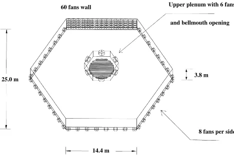
dome, before testing the aeroelastic model. The WindEEE dome, schematically shown in
Figure 2- 2, utilizes 106 individually controlled fans to simulate a variety of straight flows,
as well as axisymmetric flows like tornadoes and downbursts. Similar to conventional wind
tunnel methods, the turbulent component can be imposed using upstream flow modifiers
and about 1600 roughness blocks. The blocks are grouped into a number of sectors and
each sector can be individually controlled to reach a height between 0 and 12 inches to
3.8 m 25.0 m
14.4 m
8 fans per side Upper plenum with 6 fans
and bellmouth opening 60 fans wall
simulate target terrain exposure for a wide range of length scales. Simulation of the
downburst is performed by pressurizing the air in an upper room (called the upper plenum)
using a number of 6 fans, and then opening the vents between the upper room and the space
underneath to form the downdraft. The vents connecting the room to the space underneath
operate in a circular nozzle (called the bell mouth) as shown in Figure 2- 2. The bell mouth
allows for simulating downbursts with variable jet diameters (here it was set to 3.2 m) and
it has a height of 3.8 m from the ground. Although this leads to relatively small
diameter-to-height ratio of 1.2, such a small ratio was proven adequate for producing reliable
downburst wind field (Aboshosha et al. 2015 and Elawady et al. 2017). After
impingement, the flow convects radially until it reaches the lower peripheral, which act as
outlets by opening the louvers without the fans being operated. The downdraft speed
depends on the power input to pressurizing air in the upper plenum and it was estimated at
4-9 m/s.
A basic wind field was collected experimentally using 12 high-resolution cobra probes
distributed evenly on 2 towers as shown in Figure 2- 3 and operating at a sampling
frequency of 156 Hz. These probes were oriented towards the chamber’s centre to align the
downburst radial velocity component with the longitudinal component of the probes. Since
the flow field was characterized by only 2 towers, multiple downburst tests were conducted
while altering the tower locations. The location of the first tower is referred to as R1 and
the second tower location is referred to as R2 as shown in Figure 2- 3. The first tower was
consistently placed at the location of the maximum radial speed which was found to be at
R1=1.0 Dj. The second tower was placed at a variable distance R2 ranging between 0.7 Dj
and 3.0 Dj and at an angle theta ranging between -60 to +60 degrees. The measurements
were retaken to assess the repetitiveness of the profiles corresponding to certain fan power
and it was found satisfactory.
(a) (b)
Open and suburban terrain exposures were simulated by setting the roughness blocks at 6
and 9 inches respectively. The profiles of the mean radial velocities resulting from the
chosen block heights were compared with those simulated by Aboshosha et al. (2015) for
open and suburban exposures and have shown a good agreement as indicated in Figure 2-
4.
Highlighting the comparison discussed above, the mean component was extracted from the
time histories using a decomposition technique similar to that reported by Holmes et al.
(2008). The decomposition technique relies on the shedding frequency, where the cut-off
frequency, separating the mean and the fluctuating component, is taken as a multiple of the
shedding frequency. This technique will be discussed in more details in the following
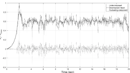
section. Figure 2- 5 shows the decomposed time history acquired using the mentioned
technique.
2.3
Numerical Model Setup
Computational Fluid Dynamic (CFD) simulations replicating the downbursts simulated at
the WindEEE dome are discussed in this section. First, details about the governing
equations and CFD solver are provided. This is followed by a description of the employed
model, boundary conditions and details of the simulation are presented.
2.3.1
LES Governing Equations
CFD models were conducted using Large Eddy Simulation (LES) due to its efficacy to
properly simulate the turbulent component and thus the transient details of the flow field.
Naiver-Stoke Equations presented by equations (2-1~2-5) are resolved at each time step
using ANSYS FLUENT solver (ANSYS Inc. 2016)) employing the dynamic sub-grid
model introduced by Germano et al. (1991) and then modified by Lilly (1992). In this
model, the model constant Cs (in equation 2-5) is computed dynamically based on the
resolved flow field and has proven to properly simulate the turbulence energy dissipation.
Pressure and velocity coupling was conducted using Pressure-Implicit with Splitting of
Operators (PISO) scheme. This scheme has proven to outperform for cells with relatively
high skewness. This usually proves worthy, although the computing time per iteration
might increase compared to the other coupling schemes. As for the spatial discretization,
the Least Squares Cell Based, Second Order and Bounded Central Differencing schemes
are used for gradient, pressure and momentum discretization respectively. Finally, for the
temporal discretization, second-order implicit time integration was chosen. These choices
were based on the recommendations and descriptions of all available schemes in the
𝜕𝑢̅𝑖 𝜕𝑡 + 𝑢̅𝑗 𝜕𝑢̅𝑖 𝜕𝑥̅𝑖 = − 1 𝜌 𝜕𝑃̅ 𝜕𝑥̅𝑖+ 𝜕
𝜕𝑥̅𝑗(−𝜏𝑖𝑗 + 2𝜈𝑆̅̅̅̅) 𝑖𝑗 (2-1)
𝜏𝑖𝑗 = 𝑢̅̅̅̅̅ − 𝑢𝑖𝑢𝑗 ̅̅̅̅̅𝑖𝑢𝑗 (2-5)
𝑆𝑖𝑗 ̅̅̅̅ = 1
2 ( 𝜕𝑢̅𝑖
𝜕𝑥̅𝑗
+𝜕𝑢̅𝑗 𝜕𝑥̅𝑖
) (2-3)
𝜏𝑖𝑗 −1
3𝛿𝑖𝑗𝜏𝑘𝑘 = −2𝜈𝑒𝑆̅̅̅̅𝑖𝑗 (2-4)
𝜈𝑒 = (𝐶𝑠Δ)2|𝐷| (2-5)
Where 𝒖, 𝒕, 𝝆, 𝑷, 𝝉, 𝝂 and 𝑺 stand for velocity, time, density, pressure, subgrid-scale
turbulent stresses, molecular viscosity coefficient and the strain rate tensor. The i, j and
k annotations represent the along, across and out-of-plane directions. 𝜈𝑒 is the eddy
viscosity, |𝑫| is the grid scale tensor, 𝚫 is the cell size and 𝑪𝒔 is the Smagronisky
constant.
2.3.2
Model Details
The computational domain was carefully constructed to include most of the elements
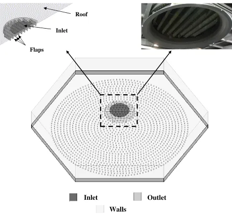
utilized in the experimental setup as shown in Figure 2- 6. This includes detailed modeling
of the inflow condition (i.e. the bell mouth with the opening flaps, roughness blocks and
the outflow condition). As shown in Figure 2- 6, the bell mouth was fully modelled with
its flaps (vents). The plenum on the other hand was spared, where a constant velocity with
synthesized turbulence inlet boundary condition with the jet diameter shall suffice to
resemble its physical role. Turbulence intensity of the downdraft was unknown during the
test since there was no cobra probe placed in the test near the bell mouth. To account for
considered and the simulation was repeated for each. It was found that the results for the
7% turbulence intensity led to the best match with the experiment as will be discussed later
in the following section.
The roughness blocks were simulated exactly as they were considered during the test. A
number of 1600 blocks was used with a block dimension of 4 x 4 inches (~10 cm x 10 cm) Roof
Inlet
Flaps
Inlet
Outlet
Walls
by either 6 or 9” (15 cm 22.5 cm) for open and suburban exposures. As for the outlet, the
geometric projection of the peripheral was modelled as a continuous surface throughout
the perimeter, where the louvers of the fans were not modelled due to their insignificance
on the flow features.
After constructing the model, ANSYS Mesher software was utilized to produce a
volumetric grid to resolve the flow. The mesh density distribution was chosen such that the
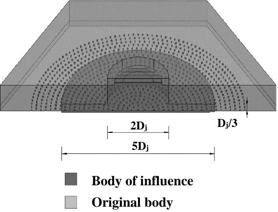
volume where the main flow develops shall have consistent grid size. Figure 2- 7 shows
the volumetric section where the influence zone was chosen. As demonstrated, the zone
was chosen to bound the core of the flow at a diameter of twice the jet diameter descending
from the inlet. Stretching beyond the jet diameter was decided to make sure the
development of vortices due to Kelvin-Helmholtz instability is fully captured within the
fine grid range. In addition, the lower segment of the domain, where the convective flow
is expected to occur, was also included in the fine grid zone. This zone was truncated at a
radial distance of 2.5 times the jet diameter for computational efficiency. Dj/3
2Dj
5Dj
Body of influence
Original body
Choosing polyhedral cells due to their efficiency in resolving rotational flows (ANSYS
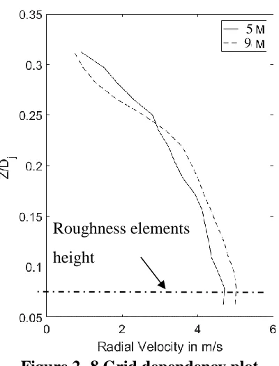
Inc. 2016), a total cell count of ~ 5 million for a cell size of Dj/64, and ~9 million for a cell
size of Dj/80 were obtained. A limited grid independence test was carried out for the two
grids based on the profiles of the maximum mean velocities. The resulting profile from
both grids is shown in Figure 2- 8, which demonstrates that both grids leads to compatible
profiles. It should be noted that the region beneath the dashed line in the figure has been
excluded from the plot, as it resembles the height that would be affected by the roughness
elements. The maximum difference between the two profiles was found less than 5%,
which indicates the grid independency of the results. It is worth to note that the coarser grid
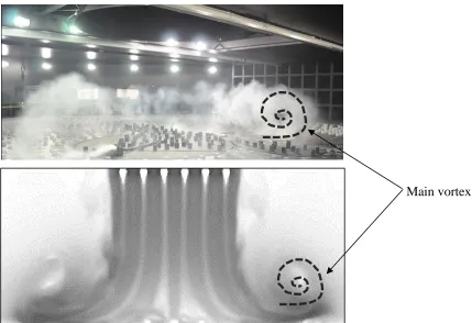
(i.e. 5 million cells) was utilized in presenting the results. Figure 2- 9 shows a comparison
between the CFD velocity contours and the experimental smoke visualization, showing the
relevance between the developed main vortex in both simulations. Roughness elements
height
Figure 2- 8 Grid dependency plot [
2.4
Results and Discussion
The CFD model described in the earlier section was utilized to obtain the wind field for the
downburst simulation and the resulting wind field is discussed in this section. First, an
overview of the transient nature of the wind field is presented, which is then followed by
describing the utilized technique to decompose the wind field into a non-stationary
“running” mean component and a turbulent component. Afterwards, a comparison between
mean and turbulent components of the wind field obtained from the CFD simulations with
those obtained from the experiment is provided.
2.4.1
Development of Wind Field
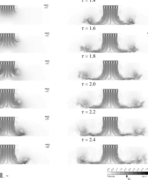
Snapshots of the velocity contours of different time instants showing how the wind field
gradually develops through the domain can be seen in Figure 2- 10. The snapshots are
Main vortex
calibrated in 𝝉, which is the time normalized by the peak radial velocity instant. At the
beginning of the simulation, when the flow is released from the inlet boundary, the
presence of the flaps with their considerable cross-section generally impacts the flow. This
can be deduced throughout the whole time range, where the flaps cause streaming of the
flow within the region of pre-impingement. The streaming limits the contribution of the
inner region of the descending downdraft to the interaction between the downdraft and the
ambient air. Such interaction can be seen in the first three time instances (i.e. 𝝉= 0.2, 0.4
and 0.6) where the Kelvin-Helmholtz instability is formed as a result of the shear between
the descending and the still air. After that, time instances beyond the impingement (𝝉 >0.8),
illustrate the radial convection mechanism, where the transported vortices are obstructed
by the roughness elements. The influence of the modelled elements can be generally
described as turbulence generators for the convecting flow. Yet, some important features
can be noticed from the figure. Firstly, the roughness elements right below the centre of
the jet can be clearly seen to entrap flow structures (𝝉> 0.6). The fact that the dimensions
of the modelled elements result in significant canopy zones can also be noted from the
displayed figure. Adding to the streaming caused by the flaps, this is believed to result in
preventing the inner core of the jet from contributing to the radial out flow after
impingement. This means that the main driving force of the outflow is generated by the
outermost part of the jet. Secondly, the main convecting vortex generally maintains its
structure throughout the monitored period, surpassing the main areas of interest located at
a jet diameter distance from the jet centre. The secondary vortex formed after impingement
due to separation, that was reported by Kim and Hangan (2007) and Aboshosha et al.
show that the newly formed structure fails to keep up with the flow and diminishes as it
encounters more roughness blocks. This can be again attributed to the size of the roughness
elements, as well as the spacing between them which is comparable to that of the formed
vortices, leading to destroying the structure of the secondary vortex. Accordingly, only the
main vortex is able to maintain its structure and carry the driving energy for the radial
convection. Thirdly, closely observing the development of the flow, secondary vortices
formed due to quasi-static Kelvin-Helmholtz instability reported by Kim and Hangan
(2007) can be noticed. These are the structures that follow the main vortex from the inlet,
later as the flow progresses. Finally, while the impact of the flaps is clearly observable in
Figure 2- 9, the roughness blocks also have a noticeable effect that can hardly be seen from
the elevation view. Figure 2- 11 representing a planar view at an elevation right above the
blocks height clearly demonstrates the effect they have on the flow. The unevenly
distributed shades are revealing the shedding, channeling and irregularity the blocks
impose on the flow. Noting that the block height is in the order of 5 and 7 percent of the
jet diameter for the open and suburban exposures respectively, the canopy zone over shades
𝜏
= 0.4
𝜏
= 1.6
𝜏
= 0.6
𝜏
= 1.8
𝜏
= 0.8
𝜏
= 2.0
𝜏
= 1
𝜏
= 2.2
𝜏
= 1.2
𝜏
= 2.4
Vj
Moreover, the plot shown in Figure 2- 12 illustrates the envelope of radial velocities
distribution throughout the entire simulation. The data plotted show that peak radial
velocities happen at a radial distance R of 1.0 Dj, a jet diameter measured from the jet
centre. Although the location of the peak wind speed happens at a closer distance to the
downdraft center compared with other simulations by Mason et al. (2009) and Aboshosha
et al. (2015a) (Rmax=1.0 Dj compared with 1.3 Dj), the obtained location well matches the
location of peak wind speed seen in the experiment.
After a close observations, it was found that the streaming effect imposed by the flaps is
the main reason that the peak radial velocity occurs at the closer radius to the center
(Rmax=1.0 Dj). Thisis relatively less than the values found in the literature, where studies
like Aboshosha et al. (2015b) and Kim and Hangan (2007) found Rmax to be in the order of
1.25~1.3. It is believed that simulating a model that follows the same physical conditions
as the previous simulations (i.e. no flaps and roughness elements with less significant
heights), Rmax would reach the same values reported by previous researchers.
2.4.2
Wind Field Decomposition
The wind field associated with downburst events is uniquely distinguished by its
non-stationarity which sets it apart from the conventional atmospheric boundary layer (ABL)
flow. While ABL is characterized by a constant mean and a zero average fluctuating
component, the downburst time history can only have a zero average fluctuating
component when the mean is itself fluctuating. This is widely agreed upon in literature,
where researchers like Holmes et al. (2008), Aboshosha et al. (2015a) and Solari et al.
(2015b) used a moving average technique to discretize the mean component from the time
history. The technique relies on an averaging window by which the time history is averaged
within the range of this moving average, resulting in a slowly varying mean, while the
residual is considered to be the zero average fluctuating component. The challenge here is
to decide upon the value of this moving average window. The chosen value shall result in
a mean component that resembles the main driving flow characteristics, without a
significant fluctuating component. Researchers like Holmes et al. (2008) and Solari et al.
(2015a) have tried different values of averaging periods, and relied on their judgement to
decide on which period could result in mean and fluctuating components that satisfy the
above criteria. Yet, researchers like Aboshosha et al. (2015a) relied on equation (2-6) to Rmax
Rmax
calculate the averaging period Tav as being a factor Xav , taken to be 0.67 in this study,
multiplied by the shedding period Tshedding. This technique with an averaging period less
than the shedding vortex assures that main vortex is included in the running mean. This
method was utilized in the current study to decompose running mean which was subtracted
from the overall wind field to obtain the turbulent component. Figure 2- 13 illustrates the
effect the factor Xav has on the mean value of the fluctuating component, which is expected
to have a near zero value for a representative fluctuating component. As shown, different
studies in the literature chose values generally smaller than unity. Although the current
study seems to yield a higher mean of the residuals, the chosen value of 0.67 still resulted
comparable results, where the mean of the fluctuating residuals is considerably small.
Furthermore, the chosen value is shown to maintain the mean characteristics as indicated
by Holmes et al. (2008) and Solari et al. (2015a), where the mean profile follows the
general characteristics of the flow as shown in Figure 2- 14. The calculated averaging
period is then applied to the velocity time history using a bi-directional moving average
filter to eliminate the lag that would shift the decomposed mean in case of uni-directional
averaging. The same technique was applied on the experimental results reported in the
previous section.
Applying the resulting moving average on the time history at a sample probe point, the
resulting time histories are shown in Figure 2- 14. As shown in the figure, the total time
history plotted contains fluctuation that was separated to a slowly varying mean, and a zero
mean fluctuation. The velocity time history data was collected using a 3 dimensional grid
of vertex averaging probes. Adding to the fact that polyhedral cells increase the accuracy
due to better approximation of gradients between neighbouring cells, averaging in between
vertices adds more confidence to the results monitored by probes.
𝑇𝑎𝑣 = 𝑋𝑎𝑣 ∗ 𝑇𝑠ℎ𝑒𝑑𝑑𝑖𝑛𝑔 (2-6)
Main vortex included
2.4.3
Mean Component of Wind Field
A comparison between the CFD and the experimental mean components of the flow is
shown in Figure 2- 15. The plot shows the decomposed mean profiles at a time instant
corresponding to the occurrence of the peak mean radial velocity. Comparison between the
CFD and the experimental data show satisfying agreement within the monitored range.
Yet, due to the impact of the roughness elements on the flow, shown in Figure 2- 11 and
discussed above, no probe points were taken below the height of the roughness blocks for
both the open and the suburban exposures. It was expected that, below the roughness
height, either shedding or channeling effects would yield misleading results. Therefore,
although being one of the key parameters for wind engineering, the height at which the
peak velocity occurs was not detected due to it being within the canopy zone of the
roughness blocks.
2.4.4
Turbulent Component of Wind Field
2.4.4.1
Turbulence Spectra
Power spectral density of the turbulence resulting from the decomposition technique
discussed earlier was generated and plotted in Figure 2- 16 at the location of the maximum
mean (i.e. Rmax=1.0 Dj) for the open and suburban terrains. Power spectral density function
of the turbulent speeds obtained from the experiment are also shown in the figure for
comparison purpose. As seen from the figure, both PSDFs are in a good agreement.
Match between CFD PSDF and experimental PSDF is up to a certain frequency, which is
the maximum frequency of the resolvable eddies by the employed computational mesh.
This maximum frequency was found equal to 7Hz. It is worth to mention that PSDF for
downburst speeds converged to the -5/3 power after a frequency of 5 (<7) Hz for both
experiential and numerical simulations. It is also important to note that the CFD predicted
Figure 2- 17 shows the area under the curve where the LES simulation could capture
frequencies (A1), compared to the area where the simulation could no longer detect
frequencies (A2). Although the current simulation used a relatively fine grid size, the ratio
between A1 to the total area (A1+A2) is about 40%. This is also evident from the plots
illustrated in Figure 2- 18, showing the turbulence intensity profiles for different turbulence
intensities specified at the inlet boundary conditions. It appears that the 7% profile gives
the best match, where the ratio between the experimental and the numerical turbulence
intensities is roughly 1.7~1.9. The plot also shows the corrected turbulence intensity profile
of the 7% inflow turbulence after correcting it with the factor of 1.8. Accordingly, the
2.4.4.2
Turbulence Intensity
Turbulence intensity (Iur) represents an important parameter that indicates the relation
between the mean and the peak values of turbulent flows. Following equation (2-7), the
turbulence intensity is generally defined as the ratio between the statistical root mean
square and the mean value of time history. Yet, the fact that the mean component of
downburst wind field is not a constant value, requires some adjustment to account for the
non-stationarity of downbursts. Accordingly, the statistical properties are calculated within
a certain range rather than the complete time history. Following Holmes et al. (2008) and
Aboshosha et al. (2015a), the turbulence intensities were calculated at time instants where
the maximum mean velocities occurred. With the time instant known, the clipped range at
which statistical properties were computed spreads one half of the averaging period before
and after the specified instance. As shown in equation (2-8), the value of the total
undecomposed velocity (𝒖(𝒕)) and the mean velocity corresponding to the considered time