Efficient implementation algorithm for a homogenized energy model with thermal relaxation

(1)

Efficient Implementation Algorithm for a

Homogenized Energy Model with Thermal Relaxation

Thomas R. Braun

∗

_{and Ralph C. Smith}

†

Center for Research in Scientific Computation / Department of Mathematics

North Carolina State University, Raleigh, NC 27695

ABSTRACT

In this paper, we present a new algorithm to implement the homogenized energy hysteresis model with thermal relaxation for both ferroelectric and ferromagnetic materials. The approach conserves most of the accuracy of the original algorithm, but enables all erfc and exp functions to be calculated in advance, thereby requiring that only basic mathematical operations be performed in real time. This is done without a significant increase in memory usage. Using this approach, execution time of the model has been seen to improve by a factor of 70 for some applications, whereas the error only increases by five ten thousandths (0.05%) of the saturation polarization/magnetization. The model with negligible relaxation is also given, as it is used to illustrate some optimizations. Emphasis is placed on the efficient computation of these models, and theoretical development is left to the references.

Keywords: Ferromagnetic, ferroelectric, thermal relaxation, thermal activation, real-time, homogenized energy, hysteresis model

1. BACKGROUND

The homogenized energy framework provides a powerful and flexible mechanism to model ferroelectric and ferromagnetic hysteresis. In this framework, Gibb’s energy minimization is considered at the lattice level, using the kernel

¯

P(E) = E

η +PRδ, (1)

whereE is the electric field, ¯P is the average polarization,PR is the polarization at remanence,η is the inverse

susceptibility,δ=₋1 for negatively oriented dipoles, andδ= 1 for those dipoles with positive orientation. For magnetic materials, the kernel is

¯

M(H) =H µ0

η +MRδ, (2)

where H is the magnetic field, M is the magnetization, MR is the magnetization at remanence, and µ0 is the

permeability. In practice, however, η is the result of a data fit, andµ0 is combined with η when performing

the parameter estimation for magnetic materials. This allows the same model to be used for both classes of materials. For simplicity, this paper refers solely to electric fields and polarizations, with the understanding that everything presented here applies not only to electric but also to magnetic materials.

To account for material nonhomogenuities and interactions between dipoles, both the coercive field value at which δ changes and the interaction field between dipoles are assumed to be manifestations of an underlying distribution. The requirements placed on these distributions are minimal: the coercive field distributionEc is

strictly non-nonnegative, the interactive field distributionEI is symmetric about 0, and both distributions are

bounded by a decreasing exponential. Including these distributions gives the model

P(E) =

Z ∞

0 Z ∞

−∞

vc(Ec)vi(EI) ¯P(E+EI;Ec)dEIdEc, (3)

(2)

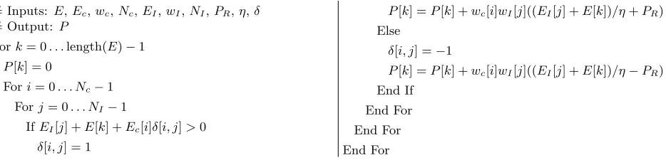
# Inputs: E,Ec,wc,Nc,EI,wI,NI,PR,η,δ

# Output: P

Fork= 0. . .length(E)₋1

P[k] = 0

Fori= 0. . . Nc−1 Forj= 0. . . NI−1

IfEI[j] +E[k] +Ec[i]δ[i, j]>0

δ[i, j] = 1

P[k] =P[k] +wc[i]wI[j]((EI[j] +E[k])/η+PR) Else

δ[i, j] =−1

P[k] =P[k] +wc[i]wI[j]((EI[j] +E[k])/η−PR) End If

End For End For End For

Algorithm 1.Algorithm used to implement the homogenized energy model with negligible thermal relaxation,

wherevc andvi represent the distributions of coercive and interaction fields, respectively. For computation, the

distribution of parameters is considered at a predetermined number of quadrature points, and in general the only restriction on the quadrature method is that an even number of quadrature points are needed on theEI

axis. This assures accurate modelling of the material in the depoled state. Implementing the quadrature method gives the model

P(E) =

Nc

X

i=1 NI

X

j=1

wc[i]wI[j] ¯P(E+EI;Ec), (4)

where Nc is the number of coercive field quadrature points, NI is the number of interaction field quadrature

points,wc=vc×coercive quadrature weights, andwI is defined similarly for the interaction field. The [ ] notation

represents array indexing. A complete discussion of the development of this model can be found in [1, 3, 2, 4], and a pseudocode implementation is given in Algorithm 1 and Table 1.

Algorithm 1 assumes the effects of thermal relaxation are negligible. Considering a material at absolute temperatureT with volumeV, the effect of thermal relaxation or activation depends on the ratiokT /V, where k is Boltzmann’s constant. When this value is very small (equivalently, when the relative lattice volume is sufficiently large), thermal relaxation is negligible and the previous model may be used. When this is not the

Name Type Description

E Vector Input electric field values – constant sampling rate assumed Ec Vector Quadrature points for coercive field distribution

wc Vector Quadrature weights times distribution levels forEc integration

Nc Scalar integer Number of coercive field quadrature points/weights

EI Vector Quadrature points for interactive field distribution

wI Vector Quadrature weights times distribution levels forEI integration

NI Scalar integer Number of interactive field quadrature points/weights

PR Scalar Polarization at remanence – determined from parameter estimation

∆t Scalar Time between successive samples ofE

η Scalar Determined from parameter estimation

β Scalar Determined from parameter estimation – Noteβ=√2kT /V

τ Scalar Determined from parameter estimation

² Scalar Small positive constant, on order of 1×10−3

f Scalar Extremely small positive constant, on order of machine accuracy limits δ Nc×NI matrix Initial state of the material – 1 if domain is positive; -1 if negative

x+ Nc×NI matrix Initial state of the material – 1 if domain is positive; 0 if negative

r Scalar integer Resolution increase for shifting operations

(3)

case, we consider the Boltzmann relation

µ(G) =Cexp

µ

−G(P)V kT

¶

, (5)

where G is the Gibb’s energy. The local average polarization is given by replacing ¯P in [4] with

¯

P(E) =x+P¯++x−P¯−, (6)

wherex+ andx− are the fraction of moments having positive and negative orientations, respectively. This can

be simplified slightly by realizing thatx− = 1−x+. The average polarizations are given by

P+= Z ∞

PI

P µ(G(P))dP, P−= Z PI

−∞

P µ(G(P))dP, (7)

wherePI is the inflection point. The moment fractions evolve according to the differential equation

˙

x+=−p+−x++p−+x−, (8)

wherep+−andp−+ represent the likelihood of dipoles switching from positive to negative and from negative to

positive, respectively. These likelihoods are given by

p+−= RPI+²

PI−² exp(−G(P)V /(kT))dP τR_P∞

I−²exp(−G(P)V /(kT))dP

, p−+=

R−PI+²

−PI−² exp(−G(P)V /(kT))dP τR−PI−²

−∞ exp(−G(P)V /(kT))dP

. (9)

Details regarding the development of these equations is given in [4], and the resulting model is implemented in Algorithm 2 with parameters as described in Table 1. Note that the calculation of these terms involves evaluating complementary error (erfc) and exponential (exp) functions. This significantly reduces the computational efficiency of the model when thermal relaxation is included.

# Inputs: E,Ec,wc,Nc,EI,wI,NI,PR,η,β,τ, ²,f,x+

# Output: P

Fori= 0. . . Nc₋1

PI[i] =PR−Ec[i]/η

End For

P[k] = 0

Fori= 0. . . Nc₋1 Forj= 0. . . NI−1

Pmin− = (E[k] +EI[j])/η−PR P+

min= (E[k] +EI[j])/η+PR

IfEc[i]−E[k]−EI[j]>0

p−+= (erfc((Pmin− +PI[i]−²)/β)−

erfc((Pmin− +PI[i] +²)/β))/

(τerfc((Pmin− +PI[i]−²)/β) +f)

Else

p−+= 1/τ

End If

IfEc[i] +E[k] +EI[j]>0

p+−= (erfc((PI[i]−²−Pmin+ )/β)−

erfc((PI[i] +²₋P+

min)/β))/

(τerfc((PI[i]−²−Pmin+ )/β) +f)

Else

p+−= 1/τ

End If

x+[i, j] =

x+[i, j] +p−+∆t

1 + ∆t(p+−+p−+)

¯

P−=−

βexp(−((−PI[i]−²−P−

min)/β)

2₎ √_πerfc₍₍_PI_[_i_{] +}_²₊_P−

min)/β) +f

+Pmin−

¯

P+=

βexp(−((PI[i] +²−Pmin+ )/β)2)

√

πerfc((PI[i] +²−P+

min)/β) +f

+P+

min

P[k] =P[k] +wc[i]wI[j](x+[i, j] ¯P++ (1−x+[i, j]) ¯P−)

End For

(4)

2. REPETITIVE OPERATIONS

In a first step to improve the efficiency of the model, several repetitive operations can be removed. For simplicity, consider first the model with negligible relaxation. For each iteration and each mesh point,

P[k] =P[k] +wc[i]wI[j] µ

EI[j] +E[k]

η ±PR

¶

(10)

must be calculated. Note thatEI does not change through the course of the algorithm, and thatdEis the same

for all mesh points in a given temporal iteration. Thus, each point inEI may be divided through byη as part

of algorithm setup, andE[k] divided just once per iteration (this division will later be removed). This process transforms (10) into

P[k] =P[k] +wc[i]wI[j](EI[j] +E[k]±PR)

=P[k] +wc[i]wI[j]EI[j] +wc[i]wI[j]E[k]±wc[i]wI[j]PR.

(11)

Note that each mesh point adds three terms toP[k]. The first,wc[i]wI[j]EI[j], is independent of the input field,

and a scalar value for P_iP_jwc[i]wI[j]EI[j] may be calculated and stored a priori. The second does depend

on the input field, but only as a scalar multiple. As such, this term can be simplified to one multiplication per temporal iteration by calculating the scalar term P_iP_jwc[i]wI[j] in advance. In actuality, we compute

(P_iP_jwc[i]wI[j]EI[j])/ηand (Pi P

jwc[i]wI[j])/η, to combine this simplification with the division mentioned

above. The final term is±wc[i]wI[j]PR, where the sign depends on the field level and the current state of the

material. This must still be done in iteration. However, we may pre-multiply eitherwc orwI byPr, and remove

a multiplication from the loop. Further, the multiplication bywc[i] need not be performed for every mesh point,

but only once per row (only when i changes). This requires accumulating the wI[j] terms into a temporary

register, but this action is typically much more efficient than a multiplication. Incorporating these optimizations into the negligible relaxation model yields Algorithm 3. While some of these changes would be done anyway by an optimizing compiler (exactly which ones depends on the compiler), most compilers would not perform all these steps, and making these changes can give a noticeable improvement in computational efficiency. We found that Algorithm 3 runs almost twice as quickly as Algorithm 1 when both were compiled under the gcc compiler with optimizations enabled. More performance comparisons may be found in Section 4.

# Inputs: E,Ec,wc,Nc,EI,wI,NI,PR,η,δ

# Output: P

# Initial Setup – not input field dependent

addit= 0

wsum= 0

Fori= 0. . . Nc−1 Forj= 0. . . NI₋1

addit=addit+wc[i]wI[j]EI[j]

wsum=wsum+wc[i]wI[j] End For

End For

addit=addit/η wsum=wsum/η

Forj= 0. . . NI−1

wI[j] =wI[j]PR

End For

# Begin Iteration

dE=E[k]₋E[0]

P[k] =addit+wsumdE

Fori= 0. . . Nc₋1

out= 0

Forj= 0. . . NI−1

IfEI[j] +dE+Ec[i]δ[i, j]>0

δ[i, j] = 1;

out=out+wI[j] Else

δ[i, j] =−1

out=out−wI[j] End If

End For

P[k] =P[k] +wc[i]out

End For End For

(5)

To remove repeated operations from the relaxation model, we do not calculate PI, Pmin− , and Pmin+ directly,

as in Algorithm 2. This change effects the equations forp−+,p+−, ¯P−, and ¯P+. For example,

p−+ =

erfc((P−

min+PI[i]−²)/β)−erfc((Pmin− +PI[i] +²)/β)

τerfc((Pmin− +PI[i]−²)/β) +f

= 1 τ

µ

1− erfc((E[k] +EI[j]−Ec[i])/(ηβ) +²/β)

erfc((E[k] +EI[j]−Ec[i])/(ηβ)−²/β) +f ¶

,

(12)

where the fact thatf is essentially 0 has been used to remove anerfccalculation. We now see that division by η andβ can be done in advance (for all terms exceptE[k]) or once per temporal iteration (forE[k]). The same holds forp+−. Further, let

¯

P−=Pb−+Pmin− =Pb−+

E[k] +EI[j]

η −PR,

b

P−=−

βexp(₋((Ec[i]−EI[j]−E[k])/(ηβ)−²/β)2) √

πerfc((−Ec[i] +EI[j] +E[k])/(ηβ) +²/β) +f

,

(13)

¯

P+=Pb++Pmin+ =Pb++

E[k] +EI[j]

η +PR,

b

P+=

βexp(₋((₋Ec[i]−EI[j]−E[k])/(ηβ) +²/β)2) √_π

erfc((−Ec[i]−EI[j]−E[k])/(ηβ) +²/β) +f

.

(14)

This allowsηandβto be divided through in advance for these equations, and simplifies the polarization relation to

P[k] =P[k] +wc[i]wI[j](x+[i, j] ¯P++ (1−x+[i, j]) ¯P−)

=P[k] +wc[i]wI[j] µ

x+[i, j] ³

b

P+−Pb−+ 2PR ´

+Pb−+ µ

EI[j]

η −PR

¶

+E[k] η

¶

. (15)

This in turn allows thewc[i]wI[j](EI[j]/η−PR) andwc[i]wI[j]E[k]/ηto be calculated in advance, as was done with

the negligible relaxation model. Incorporating these optimizations yields Algorithm 4. Numerical experiments demonstrate that Algorithm 4 runs about 15% to 20% faster than Algorithm 2 (again, more detailed results can be seen in Section 4). However, more significant then the speed increase given by Algorithm 4 is the framework it establishes for the more significant optimizations given in the next section. It should be noted that Algorithms 3 and 4 are equivalent (within numerical limits) to Algorithms 1 and 2, respectively; we have not lost any accuracy by making these changes.

3. CALCULATION OF LIKELIHOODS AND AVERAGE POLARIZATIONS

Whereas some improvement in the relaxation algorithm was gained in the previous section, Algorithm 4 is still many times slower than Algorithm 3. Much of this time is spent in calculating the erfc and exp functions, which occur in the equations for p−+, p+−, Pb−, and Pb+. Examining the equations for p−+ and Pb−, the only

non-constant terms are E[k], EI, and Ec, and these always occur together in the same pattern. As such, we

write them as a function of a single variable

Eµ =E[k] +EI[j]−Ec[i]. (16)

This givesp−+ andPb− as functions of a single variable, which are calculated as

b

P−=−

βexp(₋(₋Eµ−²)2) √

2erfc(Eµ+²) +f

(6)

# Inputs: E,Ec,wc,Nc,EI,wI,NI,PR,η,β,τ, ²,f,x+

# Output: P

²=²/β

Forj= 0. . . NI₋1

EI[j] =EI[j]/(ηβ) End For

addit= 0

wsum= 0

Fori= 0. . . Nc−1

Ec[i] =Ec[i]/(ηβ) Forj= 0. . . NI−1

End For

addit=β addit−PRwsum wsum=wsumβ

# Begin Iteration

E[k] =E[k]/(ηβ)

P[k] =addit+wsumE[k] Fori= 0. . . Nc−1

out= 0

Forj= 0. . . NI−1

tmp=erfc(E[k] +EI[j]−Ec[i] +²) IfEc[i]−E[k]−EI[j]>0

p−+=

1

τ(1−

tmp

erfc(E[k] +EI[j]−Ec[i]−²) +f)

Else

p−+=

1

τ

End If

b

P−=−

βexp(₋(₋E[k]₋EI[j] +Ec[i]₋²)2₎ √

π tmp+f tmp=erfc(₋E[k]₋EI[j]₋Ec[i] +²)

IfEc[i] +E[k] +EI[j]>0

p+−= 1

τ(1−

tmp

erfc(−E[k]−EI[j]−Ec[i]−²) +f)

Else

p+−= 1

τ

End If

b

P+=

βexp(−(−E[k]−EI[j]−Ec[i] +²)2₎ √_{π tmp}₊_f

x+[i, j] =

x+[i, j] +p−+∆t

1 + ∆t(p+−+p−+)

out=out+wI[j](x+[i, j](Pb+−Pb−+ 2PR) +Pb−) End For

End For

Algorithm 4.Implementation of the homogenized energy algorithm including thermal relaxation – repeated operations removed.

IfEµ>0

p−+=

1 τ Else

p−+=

1 τ

µ

1− erfc(Eµ+²)

erfc(Eµ−²) +f ¶

.

(18)

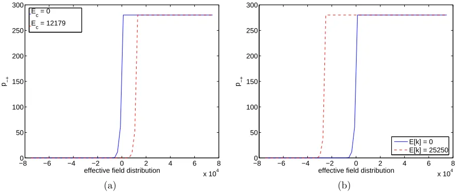
This fact is illustrated in Figure 1. Notice that changingEc,EI, orE[k] shifts the resulting likelihood function,

but does not otherwise change the shape of the function. If the solutions of (17) and (18) are known for all Eµ∈lR, then the loop iterations need only look up the the values ofp−+andPb−, rather than perform the complex

calculations on each iteration. The same process holds forp+− andPb+, except thatEµ=−E[k]−EI[j]−Ec[i].

Of course, it is impossible to calculate and store in memory the solution of (17) or (18) for all Eµ ∈ lR.

However, it is possible to bound both the range and resolution needed for Eµ, thereby obtaining a vector that

can be calculated and stored in memory. To bound the range, one of two options may be used. First, if the input field level is bounded by an arbitrary number, a minimum and maximum possibleEµ may be calculated. To

do this, we note that the minimum and maximum values of Ec and EI are known from the quadrature points.

The minima and maxima can be added together to boundEµ. A second approach to boundEµ is to recall that

the distribution forEc is bounded by a decaying exponential. As such, for Eµ > Ec[Nc−1], we may assume

(7)

−8 −6 −4 −2 0 2 4 6 8

x 104

0 50 100 150 200 250 300

effective field distribution

p−+

E_c = 0

E_c = 12179

−8 −6 −4 −2 0 2 4 6 8

x 104

0 50 100 150 200 250 300

effective field distribution

p−+

E[k] = 0 E[k] = 25250

(a) (b)

Figure 1. (a) Shift caused by a different coercive field value with 0 applied field. (b) Shift caused by different applied fields withEc= 0.

dipoles line up uniformly, the material acts as a single domain and behaves in a linear fashion as given by the kernel (1). Thus, we only need to know the values ofp−+ andPb− forEµ ∈[−Ec[Nc−1], Ec[Nc−1]]. Values

outside this range will simply give 0 forPb−andPb+ and either 0 or 1/τ forp−+ andp+− (depending on whether

the out of range value is positive or negative). The first approach yields a slightly simpler final model, but places an additional constraint on the input field level. The second approach requires no additional constraints, but does require checking for out-of-bounds values (which can never occur in the first approach). To maintain generality, the second approach is employed here, with one modification. To reduce the number of out-of-bounds calculations (at the expense of memory usage), we allowEµ∈[−Ec[Nc−1]−EI[NI−1], Ec[Nc−1] +EI[NI−1]].

As mentioned above, all the points just added to the range ofEµ will give repetitive values for the likelihoods

and average polarizations. However, given anE[k] andEc[i], we may now iterate over all values of EI, checking

only the first for an out of bounds condition. All other values that do not giveEµ ∈[−Ec[Nc−1], Ec[Nc−1]]

will receive the same out of bounds values as before, without additional conditional logic to check their bounds. We have limited the range ofEµ that must be considered, but that by itself still gives infinitely many possible

values. The resolution of Eµ must now be set. This problem should be familiar to anyone who has designed

numerical methods. The higher the resolution, the more accuracy is obtained, but the more memory is needed. If the resolution is set arbitrarily, a very large amount of memory is needed to give accurate results (potentially many tens to a couple hundred thousand points or more for each ofp−+,p+−,Pb−, andPb+). This is unacceptably

large for most real-time applications. To improve this, we must restrict the quadrature method overEI to one

of the Newton-Coates formulas (to maintain the even number of quadrature points, it must be an even degree formula such as trapezoid or Simpson’s 3/8 rule over an odd number of intervals). This restriction yields equally spaced quadrature points. The resolution can now be set as some positive integer divisorr of the EI stepsize.

Quantization error will still be introduced whenEc and E[k] are not zero; however, no additional quantization

is added by iterating overEI. This reduces the amount of error significantly. While the exact amount of error

depends on the parameters being used, in test cases we’ve run less than a thousand points need to be calculated and stored for p−+, p+−, Pb−, and Pb+ in order to limit the increased quantization error to values well below

(8)

# Inputs: E,Ec,wc,Nc,EI,wI,NI,PR,η,β,τ,², # f,x+,r

# Output: P

²=²/β addit= 0

wsum= 0

Fori= 0. . . Nc₋1 Forj= 0. . . NI−1

End For

addit=addit/eta−PRwsum wsum=wsum/eta

estep= (EI[1]−EI[0])/r Nr=NI r

IfEc[Nc₋1]> EI[EI₋1]

increase= ceil((Ec[Nc−1]−EI[NI−1])/estep) +Nr

Else

increase=Nr−floor((EI[NI−1]−Ec[Nc−1])/estep) End If

step=estep/(ηβ)

Nµ= 2increase+Nr ef f=EI[0]/(ηβ) Forj= 0. . . Nµ−1

Eµ=ef f₋step increase+step j tmp−=erfc(Eµ+²)

tmp+=erfc(−Eµ+²)

IfEµ>0

p−+[j] = 1/τ

p+−[j] = (1−tmp+/(erfc(−Eµ−²) +f))/τ

Else

p−+[j] = (1−tmp−/(erfc(Eµ−²) +f))/τ p+−[j] = 1/τ

End If

b

P−[j] =−βexp(−(Eµ+²)2)/(√π(tmp−+f)) b

P+[j] =βexp(−(−Eµ+²)2)/(√π(tmp++f))

End For

# Begin Iteration

Fork= 0. . .length(E)

P[k] =addit+wsumE[k]

kshif t=E[k]/estep

Fori= 0. . . Nc−1

ishif t=Ec[i]/estep

j−= round(increase+kshif t−ishif t) Ifj−<0 Thenj−= 0 End If

Ifj−+Nr ≥NµThenj−=Nµ−Nr−1 End If

j+= round(increase+kshif t+ishif t)

Ifj+<0 Thenj+= 0 End If

Ifj++Nr≥NµThenj+=Nµ−Nr−1 End If

out= 0

Forj= 0. . . NI₋1

j−=j−+r

j+=j++r

x+[i, j] =

x+[i, j] +p−+[j−] ∆t 1 + ∆t(p−+[j−] +p+−[j+])

out=out+wI[j](x+[i, j](P+[j+]−P−[j−] + 2PR)+

P−[j−]) End For

End For End For

Algorithm 5. Improved algorithm for the homogenized energy model with thermal relaxation.

depend on the parameters input and the compiler/hardware being used. Regardless, this is a vast improvement over the 100 times slower execution exhibited by Algorithm 4. It should also be noted that, while the EI

quadrature has been constrained to a Newton-Coates formula, Ec has not had any constraints placed on it,

other than those mentioned in Section 1. Finally, note that the choice of constraining and working alongEI is

arbitrary. An analogous model could be developed with constraints placed onEc instead.

4. PERFORMANCE AND ERROR COMPARISONS

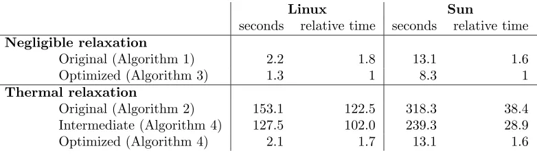
The exact performance of Algorithm 5 depends on the hardware and model parameters in use. Table 2 provides a performance comparison for an example ferroelectric material (from [3]). All five algorithms were tested with the same input of approximately 15000 field points, and used Simpson’s 3/8 rule on 21 quadrature intervals in both theEc and EI distributions (64 quadrature points). Models were compiled and run on two different platforms

(9)

Linux Sun

seconds relative time seconds relative time Negligible relaxation

Original (Algorithm 1) 2.2 1.8 13.1 1.6

Optimized (Algorithm 3) 1.3 1 8.3 1

Thermal relaxation

Original (Algorithm 2) 153.1 122.5 318.3 38.4

Intermediate (Algorithm 4) 127.5 102.0 239.3 28.9

Optimized (Algorithm 4) 2.1 1.7 13.1 1.6

Table 2.Execution time of five algorithms presented in this paper. Times are given for two different architectures.

files, and run from that environment. The first test machine used was a 1.7 GHz Pentium IV Xeon running Red Hat Enterprise Linux Workstation 3. Code on this machine was compiled with gcc 3.2.3. The other test machine was a Sunblade 100 with a 500 MHz Sparc processor. The Sun Workshop Compiler version 5.0 was used on this machine. For simplicity, these machines are referred to as linux and sun in the table.

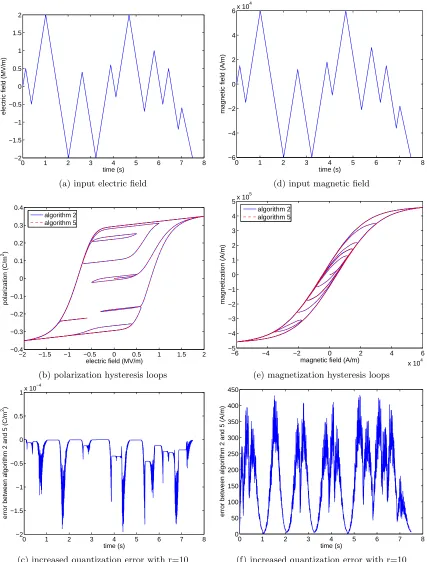
Table 2 makes it clear that Algorithm 5 is far superior computationally to a direct implementation of the homogenized energy model with thermal relaxation, as given in Algorithm 2. The test detailed in the table gives almost a 25 times improvement on the RISC-based SPARC processor, and over a 70 times improvement on the more CISC-designed Pentium IV. Tests with other parameters have yielded slightly less dramatic differences, but still give marked improvement. For example, the same Pentium IV machine gave a 25 times improvement for the computation speed of Algorithm 5 when run on an example ferromagnetic material (from [5]). The reason for this difference is believed to be related to the internal computer architecture, but is not yet fully understood. As noted before, the improved run time of Algorithm 5 is not free; increased quantization error has been in-troduced into the polarization/magnetization calculations. However, this quantization error is quite manageable. Figure 2 illustrates the input, output, and difference between the original relaxation algorithm (Algorithm 2) and the optimized one presented in this paper (Algorithm 5) for r= 10, and Table 3 gives the maximum and root mean square (RMS) error forrvalues between 1 and 64. Notice that in all cases, the maximum error introduced by the optimizations is less than 0.6% (1 part in 167) of the saturation polarization or magnetization. Further, note that error is inversely proportional tor. Thus, error can be roughly halved by doublingr. This should allow the faster algorithm to perform to almost any desired level of accuracy (when compared to the original model). A largerrhas very little effect on the computational speed of the algorithm, as it only requires accesses of larger constant arrays (p−+, p+−, Pb−, and Pb+). No significant computation difference was seen forr values of 1 to

16 in the ferroelectric example, and no significant difference was seen for anyrin Table 3 for the ferromagnetic example. However, the size of likelihood and average polarization/magnetization arrays is proportional tor, so more memory must be utilized for finer resolutions, but is still fairly small for moderater. Withr= 1, only 502

Ferroelectric Example Ferromagnetic Example

r max error RMS error max error RMS error

1 4.42_×10−4 _0.13% ₁_.₂₄_×₁₀−4 _0.035% ₂₀₀₇ _0.44% ₉₉₄ _0.22%

2 9.97_×10−4 _0.28% ₁_.₉₇_×₁₀−4 _0.056% ₂₆₆₈ _0.58% ₁₁₁₁ _0.24%

4 4.74_×10−4 _0.14% ₉_.₁₅

×10−5 _0.028% ₁₁₄₇ _0.25% ₅₀₂ _0.11%

8 2.64_×10−4 _0.075% ₄_.₇₂

×10−5 _0.013% ₅₆₁ _0.12% ₂₄₄ _0.053%

10 1.95×10−4 _0.056% ₃_.₇₃_×₁₀−5 _0.011% ₄₃₂ _0.094% ₁₉₄ _0.042%

16 1.47×10−4 _0.042% ₂_.₃₁_×₁₀−5 _0.0066% ₃₂₀ _0.070% ₁₂₁ _0.026%

32 9.30×10−5 _0.027% ₁_.₂₇_×₁₀−5 _0.0036% ₁₈₂ _0.038% _61.3 _0.013%

64 6.73×10−5 _0.019% ₇_.₇₈_×₁₀−6 _0.0022% ₁₃₆ _0.030% _33.0 _0.0072%

(10)

0 1 2 3 4 5 6 7 8 −2

−1.5 −1 −0.5 0 0.5 1 1.5 2

time (s)

electric field (MV/m)

0 1 2 3 4 5 6 7 8

−6 −4 −2 0 2 4

6x 10

4

time (s)

magnetic field (A/m)

(a) input electric field (d) input magnetic field

−2 −1.5 −1 −0.5 0 0.5 1 1.5 2

−0.4 −0.3 −0.2 −0.1 0 0.1 0.2 0.3 0.4

electric field (MV/m)

polarization (C/m

2)

algorithm 2 algorithm 5

−6 −4 −2 0 2 4 6

x 104

−5 −4 −3 −2 −1 0 1 2 3 4

5x 10

5

magnetic field (A/m)

magnetization (A/m)

algorithm 2 algorithm 5

(b) polarization hysteresis loops (e) magnetization hysteresis loops

0 1 2 3 4 5 6 7 8

−2 −1.5 −1 −0.5 0 0.5

1x 10 −4

time (s)

error between algorithm 2 and 5 (C/m

2)

0 1 2 3 4 5 6 7 8

0 50 100 150 200 250 300 350 400 450

time (s)

error between algorithm 2 and 5 (A/m)

(c) increased quantization error with r=10 (f) increased quantization error with r=10

(11)

values need to be stored for the ferroelectric example (64 quadrature points for each ofEc andEI). Atr= 10,

this value is up to 5006 values for each of the four arrays. The ferromagnetic example benefits from a maximum Ec less than the maximumEI and needs only 152 values for r = 1 and 1514 values forr= 10 (again with 64

quadrature points for each of Ec andEI). This suggests that memory (and in some cases speed as well) may

be optimized in the ferroelectric example by optimizing along Ec instead ofEI (as is mentioned at the end of

Section 3), but this is not further explored here. In either example, this level of memory is quite obtainable in most modern microprocessor or gate array devices.

The error figures were obtained by comparing the same quadrature routines in both Algorithms 2 and 5. While this provides a good measure for the quantization error introduced by the changes made herein, it does tend to ignore the biggest drawback to Algorithm 5: the restriction to Newton-Coates quadrature on the EI

distribution. The dominant factor influencing error is often the quadrature method in use. This is especially true around zero applied field where the accuracy is often most desired. Care in choosing a quadrature method is a general numerical necessity, and is not discussed in detail here. However, we note that the speed advantage of Algorithm 5 allows many more quadrature intervals to be considered while still giving a faster execution speed than Algorithm 2. More quadrature intervals do require more memory, and applications that need very high accuracy with memory constrains in the low kilobytes may need to stop their optimizations at Algorithm 4 (which uses less memory than Algorithm 2). For most applications, however, the accuracy lost in Algorithm 5 by requiring Newton-Coates quadrature may be recovered by increasing the number of quadrature intervals, while still maintaining a faster execution speed over the origin relaxation algorithm.

ACKNOWLEDGMENTS

This work supported by the United States Department of Education GAANN fellowship and the Air Force Office of Scientific Research under the grant AFOSR-FA 9550-04-1-0203.

REFERENCES

[1] A.G. Hatch, R.C. Smith and T. De, “Model development and control design for high speed atomic force microscopy,” Smart Structures and Materials 2004, Proceedings of the SPIE, Volume 5383, pp. 457–468, 2004.

[2] R.C. Smith, M.J. Dapino and S. Seelecke, “A free energy model for hysteresis in magnetostrictive transduc-ers,”Journal of Applied Physics, 93, pp. 458-466, 2003.

[3] R.C. Smith, A. Hatch, B. Mukherjee and S. Liu, “A homogenized energy model for hysteresis in ferroelectric materials: General desnity forumulation,” CRSC Technical Report CRSC-TR04-23; Journal of Intelligent Material Systems and Structures, to appear.

[4] R.C. Smith, “Smart Material Systems: Model Development,” SIAM, Philadelphia, 2005.