On the Derivation and Implementation of a Four Stage Harmonic Explicit Runge Kutta Method*

(1)

http://dx.doi.org/10.4236/am.2015.64064

How to cite this paper: Wusu, A.S., Akanbi, M.A. and Fatimah, B.O. (2015) On the Derivation and Implementation of a Four Stage Harmonic Explicit Runge-Kutta Method. Applied Mathematics, 6, 694-699. http://dx.doi.org/10.4236/am.2015.64064

On the Derivation and Implementation of a

Four Stage Harmonic Explicit Runge-Kutta

Method

*

Ashiribo Senapon Wusu

1

, Moses Adebowale Akanbi

1

, Bakre Omolara Fatimah

2

1_{Department of Mathematics, Lagos State University, Lagos, Nigeria}

2_{Department of Mathematics, Federal College of Education (Technical), Lagos, Nigeria} Email: [email protected], [email protected], [email protected]

Received 19 January 2015; accepted 22 April 2015; published 23 April 2015

This work is licensed under the Creative Commons Attribution International License (CC BY). http://creativecommons.org/licenses/by/4.0/

Abstract

In recent times, the derivation of Runge-Kutta methods based on averages other than the arith-metic mean is on the rise. In this paper, the authors propose a new version of explicit Runge-Kutta method, by introducing the harmonic mean as against the usual arithmetic averages in standard Runge-Kutta schemes.

Keywords

Explicit, Harmonic, Runge-Kutta, Autonomous

1. Introduction

During the last few decades, there has been a growing interest in problem solving systems based on the Runge- Kutta methods. Several methods have been developed using the idea different means such as the geometric mean, centroidal mean, harmonic mean, contra-harmonic mean and the heronian mean.

In previous papers [1] and [2], the authors presented a three stage method based on the harmonic mean and a multi-derivative method using the usual arithmetic mean respectively. Akanbi [3] developed a third-order me-thod based on the geometric mean. In [4] and [5], the concept of the heronian mean was introduced. Evans and Yaacob [6] introduced a fourth-order method based on the harmonic mean while Yaacob and Sanugi [7] also developed a fourth-order method which is an embedded method based on the arithmetic and harmonic mean. Wazwaz [8] presented a comparison of modified Runge-Kutta methods based on varieties of means. Using the

(2)

definition of the harmonic mean, a fourth-order Runge-Kutta method is developed and implemented.

2. Derivation of the 4sHERK Method

The schemes introduced by [7] and [9] respectively are

HM 1 2 2 3 3 4

1

1 2 2 3 3 4

2 3

n n

k k k k

k k

y y h

k k k k k k

+

 

= + _ + + _

+ + +

  (1)

where

(

)

1 n, n

k = f x y

2 1

1 1

,

2 2

n n

k = f x_ + h y + hk _

 

3 1 2

1 1 5

,

2 2 8

n n

k = f x_ + h y − hk + hk _

 

4 1 2 3

1 7 9

,

4 20 10

n n

k = f x_ +h y − hk + hk + hk _

 

and

AHM 1 2 3 4

1 2 3

1 2 3 4

1 1 2 2

6 6 3 3

n n

k k k k

y y h k k

k k k k

+

    

= +  + +  ₊ +  ₊ 

    

  (2)

where

( )

1 n

k = f y

2 1

1 2

n

k = f_y + hk _

 

3 1 2

1 5

2 8

n

k = f_y − hk + hk _

 

4 1 2 3

1 7 9

4 20 10

n

k = f_y − hk + hk + hk _

 

Scheme (2) was referred to as RK-HM-AM. Using the definition of harmonic mean, the following scheme is proposed in this paper:

(

)

1 ;

n n H n

y+ = y + Φh y h (3) where,

(

)

1 2 3 4

1 2 3 1 2 4 1 3 4 2 3 4

4 ;

H n

k k k k y h

k k k k k k k k k k k k

Φ =

+ + + (4)

( )

1 n

k = f y

(

)

2 n 21 1

k = f y +b hk (5)

(

)

3 n 31 1 32 2

k = f y +b hk +b hk (6)

(

)

4 n 41 1 42 2 43 3

k = f y +b hk +b hk +b hk (7) where b₂₁, , , , b₃₁ b₃₂ b₄₁ b₄₂ and b₄₃ are constants to be determined.

(3)

( )

2 2 2 3 3 3 4

2 21 21 21

1 1

2 6

y yy yyy

k = +f fhb f + f h b f + f h b f +O h (8)

(

)

(

)

(

)

(

)

( )

2

2 2 2

3 31 32 21 32 31 32

3

3 2 2 3 4

21 32 21 32 31 32 31 32

1 2

1 1

,

2 6

y y yy

y yy yyy

k f fh b b f h fb b f f b b f

h f b b b b b b f f f b b f O h

  = + + + _ + + _       + _ _ + + _ + + _+     (9)

(

)

(

)

(

)

(

)

2 2

4 41 42 43 21 42 31 43 32 43

2

2 2

2 41 42 43

41 42 41 43 42 43

3 3 2 2 2 2

21 32 43 21 42 31 43 32 43

21 42 41 42 43 32 43 41 42 43

31 43 32

2 2 2

1 1 1

2 2 2

y y

yy

y

k f fh b b b f h f b b b b b b f

b

b b

f b b b b b b f

h fb b b f f b b b b b b

b b b b b b b b b b

b b b b

= + + + + + +    +  + + + + +  _     + + _ + +  + + + + + +

+

(

+

)

3

(

)

3

( )

4

41 42 43 41 42 43

1

, 6

y yy yyy

b b f f f b b b f  O h

+ + + + + _+



(10)

Substituting (8), (9) and (10) into (4) and simplifying the resulting expression using MATHEMATICA (ver-sion 8.0.1) package, the coefficients of the powers of h in (4) are compared with that of the Taylors’ expan(ver-sion of ΦH

(

y hn;

)

and upon solving the resulting system of non-linear equations we have

21 31 32 41 42 43

1 1

; 0; 1; 0; 0;

2 2

b = b = b = b = b = b = ; (11) Thus, the incremental function (4) of the proposed scheme is

(

)

1 2 2 3 2 3 5 2 5 3

;

2 8 16 32 96

y yy yyy

H n y y y

ff f f f f

y h f fhf h   h  f f f 

Φ = + + _ + _+ _ + _

   

(12)

and the proposed scheme (3) is

1 2 3 4 1

1 2 3 1 2 4 1 3 4 2 3 4

4

n n

k k k k

y y h

k k k k k k k k k k k k

+ = + ₊ ₊ ₊ (13)

where

( )

1 n

k = f y

2 1

1 2

n

k = f_y + hk _

  (14)

(

)

3 n 2

k = f y +hk (15)

4 3

1 2

n

k = f_y + hk _

  (16)

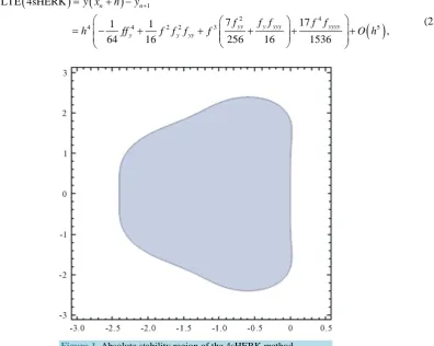
3. Stability of the 4sHERK Method

For the analysis of the absolute stability of the proposed 4sHERK scheme, the scalar test problem y′ =λy with solution y=eλy is used, where λ is a complex variable (see [10]). With the above test problem, we have

( )

1 n n

k = f y =

λ

y (17)

2 1 1 1 2 2 n n h k = f_y + hk _=λy _ + λ_

(4)

(

)

2 2

3 2 1

2

n n

h k = f y +hk =λy _ +hλ+ λ _

  (19)

2 2 3 3

4 3

1

2 2 2 4

n n

h h h

k = f_y + hk _=λy _ + λ+ λ + λ _

  _ _ (20)

Substituting (17)-(20) in (3) and simplifying the resulting expression results in,

2 2 3 3 5 5

1

1 1 1

2 8 64

n n n n n n

y₊ =y +h yλ + hλ y + hλ y − hλ y (21)

Letting z=λh and evaluating n1

n

y y

+ _{from (21), the stability polynomial of the proposed scheme is obtained as}

( )

1 1 2 1 3 1 5

( )

6

1

2 8 64

n

y

R z z z z z O z

y +

= = + + + − + (22)

The absolute stability region of the 4sHERK scheme is given inFigure 1.

4. Error Estimation

Definition: The local truncation error at x_n+₁ of the explicit one step method (3) is defined to be Tn+1 where

(

) ( )

(

( )

)

1 1 ;

n n n H n

T+ = y x+ −y x − Φh y x h

And y x

( )

_n is the theoretical solution(See [10]).

Using the above definition together with (12), the local truncation error (LTE) of the proposed scheme is given as

(

)

(

)

( )

1

2 4

4 4 2 2 3 5

LTE 4sHERK

7 17

1 1

,

64 16 256 16 1536

n n

yy y yyy yyyy

y y yy

y x h y

f f f f f

h ff f f f f O h

+

= + −

   

 

= _− + + _ + _+ _+

 

[image:4.595.134.531.400.716.2]

(23)

(5)

where y x

(

n+h

)

is obtained by Taylor series expansion.

5. Numerical Experiments

Consider the IVP

( )

1

, 0 1

y y

y

′ = = (24)

with the theoretical solution

2 1

[image:5.595.60.541.194.719.2]

y= x+ (25)

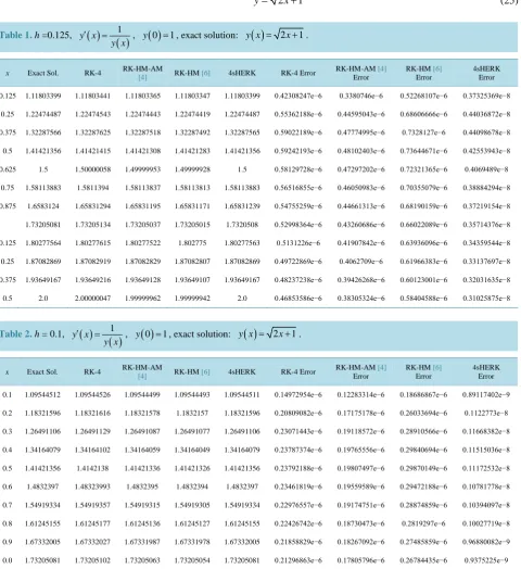
Table 1. h =0.125,

( )

1

y x y x

′ = , y

( )

0 =1, exact solution: y x

( )

= 2x+1.

x Exact Sol. RK-4 RK-HM-AM

[4] RK-HM [6] 4sHERK RK-4 Error

RK-HM-AM [4]

Error

RK-HM [6] Error

4sHERK Error 0.125 1.11803399 1.11803441 1.11803365 1.11803347 1.11803399 0.42308247e−6 0.3380746e−6 0.52268107e−6 0.37325369e−8

0.25 1.22474487 1.22474543 1.22474443 1.22474419 1.22474487 0.55362188e−6 0.44595043e−6 0.68606666e−6 0.44036872e−8 0.375 1.32287566 1.32287625 1.32287518 1.32287492 1.32287565 0.59022189e−6 0.47774995e−6 0.7328127e−6 0.44098678e−8 0.5 1.41421356 1.41421415 1.41421308 1.41421283 1.41421356 0.59242193e−6 0.48102403e−6 0.73644671e−6 0.42553943e−8 0.625 1.5 1.50000058 1.49999953 1.49999928 1.5 0.58129728e−6 0.47297202e−6 0.72321365e−6 0.4069489e−8 0.75 1.58113883 1.5811394 1.58113837 1.58113813 1.58113883 0.56516855e−6 0.46050983e−6 0.70355079e−6 0.38884294e−8 0.875 1.6583124 1.65831294 1.65831195 1.65831171 1.65831239 0.54755259e−6 0.44661313e−6 0.68190159e−6 0.37219154e−8 1.73205081 1.73205134 1.73205037 1.73205015 1.7320508 0.52998364e−6 0.43260686e−6 0.66022089e−6 0.35714376e−8 0.125 1.80277564 1.80277615 1.80277522 1.802775 1.80277563 0.5131226e−6 0.41907842e−6 0.63936096e−6 0.34359544e−8 0.25 1.87082869 1.87082919 1.87082829 1.87082807 1.87082869 0.49722869e−6 0.4062709e−6 0.61966383e−6 0.33137697e−8 0.375 1.93649167 1.93649216 1.93649128 1.93649107 1.93649167 0.48237238e−6 0.39426268e−6 0.60123001e−6 0.32031635e−8 0.5 2.0 2.00000047 1.99999962 1.99999942 2.0 0.46853586e−6 0.38305324e−6 0.58404588e−6 0.31025875e−8

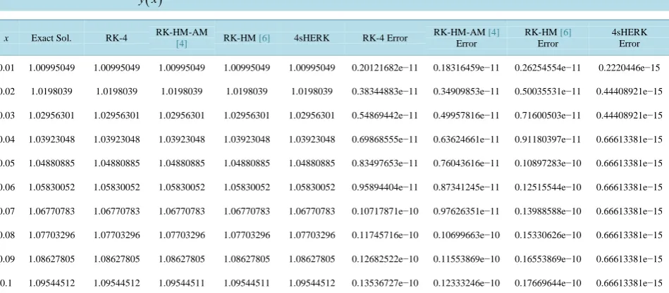
Table 2.h = 0.1,

( )

1

y x y x

′ = , y

( )

= 2x+1.

RK-HM-AM [4]

Error

RK-HM [6] Error

(6)

[image:6.595.62.537.105.313.2]

Table 3. h = 0.01,

( )

1

y x y x

′ = , y

( )

= 2x+1.

RK-HM-AM [4]

Error

RK-HM [6] Error

4sHERK Error 0.01 1.00995049 1.00995049 1.00995049 1.00995049 1.00995049 0.20121682e−11 0.18316459e−11 0.26254554e−11 0.2220446e−15 0.02 1.0198039 1.0198039 1.0198039 1.0198039 1.0198039 0.38344883e−11 0.34909853e−11 0.50035531e−11 0.44408921e−15 0.03 1.02956301 1.02956301 1.02956301 1.02956301 1.02956301 0.54869442e−11 0.49957816e−11 0.71600503e−11 0.44408921e−15 0.04 1.03923048 1.03923048 1.03923048 1.03923048 1.03923048 0.69868555e−11 0.63624661e−11 0.91180397e−11 0.66613381e−15 0.05 1.04880885 1.04880885 1.04880885 1.04880885 1.04880885 0.83497653e−11 0.76043616e−11 0.10897283e−10 0.66613381e−15 0.06 1.05830052 1.05830052 1.05830052 1.05830052 1.05830052 0.95894404e−11 0.87341245e−11 0.12515544e−10 0.66613381e−15 0.07 1.06770783 1.06770783 1.06770783 1.06770783 1.06770783 0.10717871e−10 0.97626351e−11 0.13988588e−10 0.66613381e−15 0.08 1.07703296 1.07703296 1.07703296 1.07703296 1.07703296 0.11745716e−10 0.10699663e−10 0.15330626e−10 0.66613381e−15 0.09 1.08627805 1.08627805 1.08627805 1.08627805 1.08627805 0.12682522e−10 0.11553869e−10 0.16553869e−10 0.66613381e−15 0.1 1.09544512 1.09544512 1.09544511 1.09544511 1.09544512 0.13536727e−10 0.12333246e−10 0.17669644e−10 0.66613381e−15

We apply the new 4sHERK method (13) to the above IVP and the results obtained are compared with the classical 4-stage fourth-order Runge-Kutta method and the methods of [6] and [4].

The results generated by the newly derived scheme in this paper evidently proved the extent of accuracy of the scheme in comparison with the other methods.

6. Conclusion

Evidently, the newly derived scheme is more accurate as seen from the computational results presented inTable 1,Table 2 andTable 3, since its absolute error is the least of all the methods presented in this paper. It therefore follows that the scheme is quite efficient. We therefore conclude that the 4sHERK method proposed is reliable, stable and with high accuracy in computation.

References

[1] Wusu, A.S., Okunuga, S.A. and Sofoluwe, A.B. (2012) A Third-Order Harmonic Explicit Runge-Kutta Method for Autonomous Initial Value Problems. Global Journal of Pure and Applied Mathematics, 8, 441-451.

[2] Wusu, A.S. and Akanbi, M.A. (2013) A Three-Stage Multiderivative Explicit Runge-Kutta Method. American Journal of Computational Mathematics, 3, 121-126.

[3] Akanbi, M.A. (2011) On 3-Stage Geometric Explicit Runge-Kutta Method for Singular Autonomous Initial Value Problems in Ordinary Differential Equations. Computing, 92, 243-263.

[4] Evans, D.J. and Yaacob, N.B. (1995) A Fourth Order Runge-Kutta Method Based on the Heronian Mean Formula. In-ternational Journal of Computer Mathematics, 58, 103-115.

[5] Evans, D.J. and Yaacob, N.B. (1995) A Fourth Order Runge-Kurla Method Based on the Heronian Mean. International Journal of Computer Mathematics, 59, 1-2.

[6] Evans, D.J. and Yaacob, N.B. (1993) A New Fourth Order Runge-Kutta Formula Based on Harmonic Mean. Depart-ment of Computer Studies, Loughborough University of Technology, Loughborough.

[7] Yaacob, N. and Sanugi, B. (1998) A New Fourth-Order Embedded Method Based on the Harmonic Mean. Matematica,

Jilid, 1998,1-6.

[8] Wazwaz, A.M. (1994) A Comparison of Modified Runge-Kutta Formulas Based on Variety of Means. International Journal of Computer Mathematics, 50, 105-112.

[9] Sanugi, B.B. and Evans, D.J. (1993) A New Fourth Order Runge-Kutta Method Based on Harmonic Mean. Computer Studies Report, Louborough University of Technology, UK.