Development of Vessel Lower Head Heat Transfer Analysis Capability for Evaluation of In-Vessel Retention Thermal Margin

(1)

ABSTRACT

COLMER, WILLIAM DONALD LOUIS. Development of Vessel Lower Head Heat

Transfer Analysis Capability for Evaluation of In-Vessel Retention Thermal Margin. (Under the direction of Dr. Nam Dinh).

In-vessel Retention (IVR) is a leading strategy for severe accident management (SAM) strategy in several advanced Light Water Reactor (LWR) designs. IVR strategy relies on maintaining coolability of molten corium and debris in a reactor pressure vessel lower head by external reactor vessel cooling (ERVC) by ensuring the thermal margin to critical heat flux (CHF) on the exterior. In this strategy, the integrity of the lower head is preserved and the molten corium material will remain contained in the pressure vessel, arresting

accident progression and mitigating consequences. Multiple studies have investigated boiling heat transfer on the vessel lower head exterior surface, the composition of corium layers inside the vessel, as well as the heat transfer driven by decay heating that occurs within.

The goal for this work is to develop an analytical capability to characterize heat transfer in the lower head of the corium pool layers, the vessel structure, and the heat removal on the vessel exterior. Previous work includes the FIBS model from UCSB,

followed by the VESPA revision model from INEEL and ERI IVRAM model. In this study, a lumped parameter approach is employed for heat transfer in a two-layer configuration, while the vessel lower head wall.is treated with angular segmentation to reflect large angular dependency of corium pool’s downward heat flux. This model enables thermal loading analysis in different vessel lower head geometries and input conditions, offers a vast improvement of computational time over high-resolution methods, and determines the thermal margin to vessel failure in a given scenario. The IVRAM calculations performed by Esmaili et al. are used for benchmarking the code developed in this work.

(2)

(3)

(4)

Development of Vessel Lower Head Heat Transfer Analysis Capability for Evaluation of In-Vessel Retention Thermal Margin

by

William Donald Louis Colmer

A thesis submitted to the Graduate Faculty of North Carolina State University

in partial fulfillment of the requirements for the degree of

Master of Science

Nuclear Engineering

Raleigh, North Carolina 2015

APPROVED BY:

_______________________________ ______________________________

Nam Dinh, Ph.D. Joseph M. Doster, Ph.D.

Committee Chair

________________________________ ________________________________

(5)

ii

DEDICATION

(6)

iii

BIOGRAPHY

The author graduated from Vanderbilt University in Nashville, Tennessee, with a Bachelor of Engineering degree in Mechanical Engineering in 2011. During his

(7)

iv

ACKNOWLEDGMENTS

I would like to first thank Dr. Nam Dinh for his constant guidance and support throughout our time working together. I have nothing but the deepest gratitude for your time and effort throughout the many ups and downs of this process. I would also like to thank my committee of Dr. Mike Doster, Dr. Igor Bolotnov, and Dr. Tiegang Fang for their

contributions in reviewing my work as well as two additional faculty members, Dr. John Mattingly and Dr. Steve Shannon for their advice and support throughout my graduate career. Additionally, I would like to thank the Babcock & Wilcox Company for their support and resources concerning the SMR applications of this project as well as the representatives from B&W and the Westinghouse Company who supplied aid, feedback, or additional resources used in this report.

(8)

v

TABLE OF CONTENTS

LIST OF TABLES ... vii

LIST OF FIGURES ... ix

LIST OF NOMENCLATURE ... xi

1 INTRODUCTION ...1

1.1 Background on SAM and IVR ... 1

1.2 IVR Metrics: Critical Heat Flux & Thermal Margin ... 4

1.3 Melt Pool Formation and Heat Transfer Overview ... 4

1.4 Example Safety Case & Role of IVR in SAM: Westinghouse AP1000® [3] [4] . 7 1.5 SMR Design, Safety, and Coolability ... 9

1.6 Motivations and Project Goals ... 11

2 MODEL DEVELOPMENT ...12

2.1 Literature Review ... 12

2.1.1 DOE Research, FIBS Model (Theofanous et al., 1996) [8] ...12

2.1.2 INEEL Revision, VESPA Model (Rempe et al., 1997) [9] ...13

2.1.3 ERI Study, IVRAM Model (Esmaili et al., 2005) [7] ...15

2.2 Equation Derivation ... 16

2.2.1 General Equation Derivation ...17

2.2.2 Oxide Pool ...18

2.2.3 Metallic Layer ...20

2.3 Model Equations and Parameters ... 23

2.3.1 General Parameters ...23

2.3.2 Oxide Pool ...24

2.3.3 Metallic Layer ...25

2.4 Modeling Assumptions ... 26

2.5 Correlations ... 27

(9)

vi

2.6.1 Material Properties & Geometry ...32

2.6.2 Dimensionless Numbers & Angular Position Correlation ...35

2.6.3 CHF Correlation ...37

2.7 Solution Procedure ... 38

3 VERIFICATION AND VALIDATION...41

3.1 V&V Importance and Benchmarks ... 41

3.1.1 Accuracy Verification ...42

3.1.2 Reliability Verification ...48

3.2 Model Comparison with IVRAM ... 51

3.2.1 Heat Flux and CHF Limit ...53

3.2.2 Crust and Vessel Thickness ...54

4 REACTOR APPLICATION ...55

4.1 AP1000 Results ... 55

4.1.1 Overview ...55

4.1.2 Selected Cases - Case H1 and E1 [Base Case] ...57

4.1.3 Selected Cases - Case H2 and E2 [Doubled Decay Heat] ...59

4.1.4 Selected Cases - Case H6 and E6 [Double Metallic Layer Failure] ...61

4.1.5 Selected Cases - Case H7 and E7 [Focusing Effect] ...63

4.2 SMR Results... 65

4.3 Quasi-Transient Results ... 66

4.3.1 Case QT-1 [Basic Metallic Mass Addition] ...69

4.3.2 Case QT-2 [Varied Mass Addition to Both Layers] ...70

4.3.3 Case QT-3 [Six Hour Post-Accident Timing] ...71

4.3.4 Case QT-4 [Six Hour Timing, Faster Mass Addition] ...72

4.4 Correlation Comparison ... 73

4.5 Future Work ... 78

5 CONCLUSIONS ...79

REFERENCES ...82

(10)

vii

LIST OF TABLES

Table 2-1: General parameter list ... 23

Table 2-2: Oxide pool parameter list ... 24

Table 2-3: Oxide pool equation list ... 24

Table 2-4: Metallic layer parameter list ... 25

Table 2-5: Metallic layer equation list ... 25

Table 2-6: List of correlations used ... 30

Table 2-7: Geometric equation set ... 34

Table 3-1: Summary of analytically derived values ... 44

Table 3-2: Input summary from one-layer analytic modelled case ... 47

Table 3-3: Results summary from one-layer analytic modelled case ... 48

Table 3-4: Analytic and model comparison with error calculation ... 48

Table 4-1: Base values and case parameter summary for AP1000 results ... 56

Table 4-2: Case H1 and E1 Parameters ... 57

Table 4-6: Run parameters for SMR geometry comparison study ... 66

Table 4-7: Quasi-transient parameter summary for case QT-1 ... 69

Table 4-11: Correlations used in comparison study ... 73

(11)

viii

Table 7-9: Material properties ... 95

(12)

ix

LIST OF FIGURES

Figure 1-1: AP1000 during core-coolant injection accident phase ... 2

Figure 1-2: AP1000 following core breakdown and containment cavity flooding ... 3

Figure 1-3: Decay heating curve following reactor trip... 5

Figure 1-4: Typical heat transfer scheme of stratified corium pool during ERVC ... 6

Figure 1-5: Integral SMR pressure vessel layout ... 10

Figure 2-1: Hemispherical lower head showing heat-flux and temperature profile ... 16

Figure 2-2: Generic conduction scenario ... 17

Figure 2-3: Chawla-Chan correlation visualization ... 29

Figure 2-4: Comparison of angular dependence correlations ... 36

Figure 2-5: Multipliers of ULPU configuration III CHF correlation ... 37

Figure 2-6: Sample Newton method (x0 = 2.5) ... 40

Figure 3-1: Hemispherical lower head showing heat-flux and temperature profile ... 43

Figure 3-2: Case H1 with 24 oxide pool nodes and 16 metallic layer nodes... 49

Figure 3-5: Comparison of IVRAM and NCSU heat flux to water results ... 53

Figure 3-6: Comparison of IVRAM and NCSU CHF margin results ... 53

Figure 3-7: Comparison of IVRAM and NCSU crust thickness results ... 54

Figure 3-8: Comparison of IVRAM and NCSU vessel thickness results ... 54

Figure 4-1: Results for cases H1 and E1 thermal margin to CHF ... 57

Figure 4-2: Results of case H1 heat flux to coolant by vessel position ... 58

Figure 4-3: Results for case H1 vessel thickness by vessel position ... 58

Figure 4-5: Results for case H2 heat flux to coolant by vessel position ... 60

Figure 4-6: Results of case H2 vessel thickness by vessel position ... 60

(13)

x

Figure 4-12: Results for case H7 vessel thickness by vessel position ... 64

Figure 4-13: Comparison of SMR geometries and respective thermal margins ... 65

Figure 4-14: Quasi-transient analysis of CHF ratio and layer masses for case QT-1 ... 69

Figure 4-18: Analysis of model sensitivity to Nusselt correlation ... 74

Figure 4-19: Upward facing Nusselt number in OX pool for various correlations ... 75

Figure 4-20: Downward facing Nusselt number in OX pool for various correlations ... 76

Figure 4-21: Energy splitting comparison for various correlations ... 77

Figure 4-22: Example minimum thermal margin progression over time for selected conditions ... 78

(14)

xi

LIST OF NOMENCLATURE

AP1000 – Westinghouse AP1000® Two-Loop, Generation III+ PWR (3415 MWt) AP600 – Westinghouse AP600® Two-Loop, Generation III PWR (1940 MWt) ATWS – Anticipated Transient without Scram

BWR – Boiling Water Reactor CDF – Core Damage Frequency CFP – Containment Failure Probability CHF – Critical Heat Flux

DCD – Design Control Document DNB – Departure from Nucleate Boiling ERVC – External Reactor Vessel Cooling FCI – Fuel-Coolant Interaction

HPME – High Pressure Melt Ejection HRA – Human Reliability Analysis IV(M)R – In-Vessel (Melt) Retention LERF – Large Early Release Frequency LOCA – Loss of Coolant Accident LRF – Large Release Frequency

MCCI – Molten Corium-Concrete Interaction PRA – Probabilistic Risk Assessment

PWR – Pressurized Water Reactor R(P)V – Reactor (Pressure) Vessel RCS – Reactor Coolant System SAM – Severe Accident Management

(15)

1

1 INTRODUCTION 1.1 Background on SAM and IVR

Following the nuclear accident at Fukushima Daiichi in March of 2011, the nuclear safety community has bolstered research into severe accident management and passive safety systems. This response is similar to how research into design basis accident response increased following the WASH-1400 report of 1975 and the Three Mile Island accident of 1979. The increased effort is necessary not only for preventing mistakes and oversights of the past but for determining the unrealized threats and providing a prevention strategy incorporating natural processes, risk assessment, and minimal human operator intervention. This work aims to support a small portion of that goal by characterizing a key physic during severe accident scenarios, heat transfer of molten core materials, and utilizing the results to inform the in-vessel retention severe accident management strategy.

Severe accident management strategies are often concerned with the protection of the integrity of the three basic barriers between radioactive core fission products and the general environment: the fuel rod cladding enclosures, the reactor pressure vessel, and finally the reactor containment structure. A SAM strategy changes priorities as these barriers fail in order to terminate the accident progression as soon as possible. The ultimate goal is to prevent a “large early release” of radioactive fission products into the

environment where large refers to an amount which may inflict a threshold level of casualties while early refers to a time scale that restricts or prevents evacuation or other emergency preparation efforts. Before a discussion of the varied strategies to achieve this goal, we must define a basic accident progression.

During an accident scenario excessive heat buildup, generally caused from a loss of local cooling, may cause core materials to exceed cladding melting temperatures. In order to prevent the failure of this first barrier, methods such as coolant injection into the pressure vessel may be utilized.

(16)

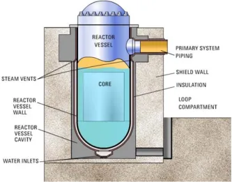
2 (corium) may continue to break down other internal structures leading to an accumulation of corium in the lower head of the RPV.

Figure 1-1: AP1000 during core-coolant injection accident phase

Following core breakdown, exposed fuel materials can react with coolant inside the pressure vessel in what is known as molten fuel-coolant interaction (MFCI). This process can generate excess heat which can further endanger the vessel structure. Inside the vessel, the molten corium collects and stratifies into distinct material layers. The main two layers to consider are the heavier ceramic and oxide materials and the lighter metallic materials from internal structures and other sources. The sole heat source in this example may be assumed as the volumetric heat generation in the oxide layer, and to a lesser extent the metallic layer, due to residual decay heat of the UO2 and subsequent fission products. This generated heat imposes a heat flux on the vessel exterior where convective cooling

(17)

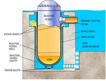
3 Figure 1-2: AP1000 following core breakdown and containment cavity flooding

At this stage, shown in Figure 1-2, successful cooling of the exterior leading to the termination of accident progression while containing all such molten corium materials within the reactor vessel is the criteria for the SAM strategy known as in-vessel melt retention. If, however, the corium remains inadequately cooled, the RPV integrity may be compromised, causing a deposit of core materials on the concrete containment basemat, the final defense between the hazardous fission products and the general environment. As IVR has failed, the next goal would be the successful cooling of the materials before the

containment barrier fails, known as ex-vessel melt retention. The focus of this document, however, is IVR and its success or failure in various accident scenarios.

NB: Figure 1-1 and Figure 1-2 are frames from an animation from the

Westinghouse Electric Company (LLC), used with permission from Mr. Jim Scobel,

(18)

4

1.2 IVR Metrics: Critical Heat Flux & Thermal Margin

In 1979, the Three Mile Island (TMI-2) accident showcased the possibility of partial or full core relocation during a loss of cooling scenario. Fortunately, only the first barrier was compromised in that accident and the progression was terminated with all materials still contained in the pressure vessel. Since the incident, however, IVR has become a key focus area for severe accident research as part of a total defense in depth strategy for facing emergency situations.

In order to adequately cool the core materials in the lower head, the containment structure must be flooded up to and exceeding the level of corium within the vessel. Once the containment and RPV have been depressurized, natural circulation provides the

convective cooling on the vessel exterior. At this point, the key physic in determining IVR success is the generated heat flux compared to the heat removal rate of the bulk fluid. In order to maintain nucleate boiling on the surface of the vessel, the heat flux value must remain below that of the critical heat flux (CHF). At this point, the system would undergo a boiling crisis, where vapor bubbles no longer detach from the vessel surface. These

bubbles, rather, accumulate into large bubble masses or entire vapor films which effectively insulate the vessel surface from the moving fluid coolant layer. Due to the inferior heat removal caused by the presence of the vapor layer, the surface temperature will rapidly rise. Once temperatures reach the melting point of the vessel, the RPV will fail locally, causing an egression of the melt and ending the IVR process. Therefore, accurate predictions of both CHF and vessel heat flux values are necessary for determining the

thermal margin or the disparity between the two values. This thermal margin will serve as the figure of merit for this project.

1.3 Melt Pool Formation and Heat Transfer Overview

As previously mentioned, as the melt pool relocates and continues to grow, it will stratify into different material layers as shown in Figure 2-1. There are important

(19)

5 however, and for the purposes of this document we shall continue to the case where the corium has begun to settle in the base of the vessel [1].

The heat in an IVR scenario may be assumed as purely decay heating of fission products contained in one or both of the stratified corium layers. Immediately following a reactor trip and control rod insertion, total decay heating drops to around 7% of previous operating levels. As is shown in Figure 1-3, heat generation drops logarithmically over time with typical accident scenarios occurring at around 0.5-1.5% of a plant’s thermal power rating. In the case of the AP1000 this accounts to approximately 15-50 MWt generated in the corium layers.

Figure 1-3: Decay heating curve following reactor trip

In the bulk of the oxide layer and in the entirety of the molten light metal layer, the primary heat transfer mechanism is natural convection driven by the internal heat

(20)

6 structures of the pressure vessel. The convection in both the oxide and metallic layers may be correlated based on the internal Rayleigh numbers and, occasionally, factor in the fluid Prandtl number when calculating the Nusselt number for the layer. Generally the heat transfer in these layers is divided into upward and downward (or sideways) facing heat fluxes. It has been shown that the sideways facing heat flux has an angular distribution, increasing as the angle from the bottom center of the vessel increases. Figure 1-4 shows a typical stratified melt pool and the associated heat transfer phenomena for the separate materials and locations. Graphic used with permission from Dr. R.R. Nourgaliev [2].

Figure 1-4: Typical heat transfer scheme of stratified corium pool during ERVC

(21)

7 fluxes may be observed at the corners of the layers. This trend is useful in predicting failure locations as well as qualitatively judging modeling results.

There are multiple uncertainties involved in the determination of the melt pool convection. The degree of stratification in the lower section of the pool determines the conduction dominant effects observed in the area. Meanwhile, the fluid properties drive the formulation of the internal Rayleigh number, which is indicative to the degree of

turbulence observed in the convective bulk of the pool. Therefore, the composition of the pool and the formation process become key physics in determining the convective flow in the layer. Uncertainties related to these physics are numerous and include the timing of the accident, the amount of coolant in the pressure vessel at the time of the first core relocation, and the method of relocation including possible jet diameter.

A separate phenomenon which occurs in the heat transfer model is that of the metallic layer focusing effect. A gross majority of the heat in the metallic layer has been received from the oxide pool as only a fraction of the corium decay heat is generated in the top layer. Since the lower thermal boundary of the metallic layer is entirely incoming heat, the transfer must occur either out of the top of the pool via radiation or through the vessel wall via conduction at the sides of the layer. When the metallic layer is fairly thin,

however, the low surface area on the sides of the pool create demonstrably higher heat fluxes than are generally seen elsewhere in the scenario. These adversely high heat fluxes can easily surpass CHF values and cut through the vessel wall if not accounted for

properly.

1.4 Example Safety Case & Role of IVR in SAM: Westinghouse AP1000® [3] [4]

The Westinghouse AP1000 is a base case example of a reactor design using similar ERVC procedures as part of its SAMG. Following is a summary of the probabilistic risk assessment (PRA) submitted by Westinghouse as part of the AP1000 DCD [5]. Also contained is an overview of the role of IVR in this safety case.

(22)

8 compiled, it is categorized based on various factors such as plant response or possible accident outcome. These initiating events then provide a basis for event trees documenting the possible accident progression. For the AP1000, 26 initiating events were categorized into three primary sections: LOCA-type events, transients, and ATWS events. Throughout the event tree process, probabilistic distributions provide likelihoods for multiple

progression factors ultimately resulting in effective expected values for each end-state in the PRA 1 process. These end-state probabilities are also subject to HRA tests in order to determine the effect of operators on stages of progression.

Once the end states have been determined through the PRA 1, the PRA 2 process takes over to determine the LRF of each PRA 1 end-state. Much like in PRA 1, the end results of PRA 2 can be classified into six main categories corresponding to the magnitude and type of release expected in each case. Not included in the LRF are scenarios resulting in a non-failed/non-bypassed containment; these cases are referred to as "no emergency action" cases. Throughout the PRA 2 process, additional probabilistic distributions and HRA tests are utilized in order to analyze pertinent severe accident phenomena. For the AP1000, the phenomena considered were: FCI/steam explosion, HPME, MCCI, and hydrogen combustion/detonation. Following the end results of PRA 2, the effects on environment, population, logistics for cleanup/evacuation, and long term effects are included in PRA level 3. In conclusion, the AP1000 PRA reported a total core damage frequency (CDF) value of 5.09x10-7/year and a total large early release frequency (LERF) of 5.94x10-8/year. Both of these values are between two to three orders of magnitude smaller than the safety goals presented by the NRC at the time of submission.

The role of IVR in the above safety case involves the mitigation of the accident progression during the PRA 2 phase. During this phase, core damage has been determined and certain event tree items such as successful depressurization of the vessel and flooding of the containment cavity signal the beginning of IVR methods. It is at that point where predictive modeling capability for key physics such as thermal margin, heat flux

(23)

9 the vessel during the IVR phase may be determined within a certain confidence. Therefore, the advancement of these methods and the improvement of the analytic capabilities for not only the single key physics but also the integrated effect allows higher confidence risk assessments and better understanding for the overall LERF.

1.5 SMR Design, Safety, and Coolability

Small modular reactor (SMR) designs focus on smaller form-factor, lower power reactor designs, typically designed with a fully passive safety system. These reactors are attractive to population areas where factors such as energy consumption, access to sufficient fresh water, or capital cost render larger plants such as the AP1000 infeasible. SMRs have also been offered as a means to retrofit coal power facilities and slowly reduce the dependence on coal in the power grid. The SMR to be examined in the project is the Babcock and Wilcox mPower design, currently in the design certification process with the USNRC. Data and information comes from publicly published sources such as Halfinger [6].

Numerous design features in the mPower reactor naturally prevent or greatly reduce key design basis accident scenarios. Reproduced in Figure 1-5, the mPower features a fully integral design where the core, once-through steam generator, control rod structure, and coolant pumps all reside within the pressure vessel housing. This structure has no

penetrations in the lower head, preventing failure modes associated with such penetrations such as instrumentation and guide tube failure (IGTF). There are also no steam or coolant lines below the level of the core, effectively preventing LOCA-type accidents.

Additionally, the control rod structures are located within the pressure vessel which prevents the pressure differential required for a rod ejection event. The plant uses standard fuel enrichment of <5% U235 and operates on a 4-year refueling cycle at which point all core materials are fully exchanged. The core balance for such a fuelling pattern produces lower average linear power densities than in conventional reactors, which improves thermal margins to CHF.

(24)

10 structure is flooded and the reactor is cooled via natural circulation for up to three days. Following a slow depressurization of the vessel, the core remains externally covered with coolant and, if the core begins to break down, the system follows an IVR strategy.

Differences in the reactor design that impact heat transfer characterization in the lower head during IVR include a lower thermal power rating of 530 MWt, lower total core and structure loading for melt pool formation, and an elliptical lower head geometry which creates a flatter and more evenly distributed platform for the corium pool.

Figure 1-5: Integral SMR pressure vessel layout Pressurizer Assembly

& Upper Head

Once – Through Steam Generator

(25)

11

1.6 Motivations and Project Goals

Previous sections discussed the necessity for accurately predicting the thermal margin to critical heat flux for the determination of IVR success. In order to obtain the most detailed and accurate view of the heat transfer scenario, high resolution methods may be used to model the lower head system. These methods are extremely computationally expensive, however, and, as a result, have exceedingly long runtimes to produce a solution for a single scenario. When considering the highly dynamic environment of a severe accident as well as the multitude of influencing factors for the heat transfer profile of the vessel, it is vital to have an accurate yet reconfigurable tool to perform multiple

calculations and simulations in a given time period. Therefore, the aim of this project is to develop a new analytic model to characterize the heat transfer in the lower head of a reactor vessel during IVR scenarios. The framework for the model is based on work performed by Esmaili et al. (IVRAM) [7] as well as previous work done by Theofanous et al. (FIBS) [8] at UCSB and Rempe et al. (VESPA) [9] at INEEL. Specifically, the model characterizes the heat transfer in a Westinghouse AP-1000 reactor undergoing natural circulation following a reactor cavity flood.

In order to provide new and useful additions to IVR analysis, there are certain characteristics desired of the final design. The goals of the model are:

1. Show a developed analytic capability for characterization of heat transfer throughout a developed corium pool and determination of the thermal margin to critical heat flux on the vessel exterior

2. Provide the above analysis for different plant properties and vessel

geometries, ultimately correlating to conventional and SMR reactor designs 3. Showcase alternative applications including quasi-transient behavior and

development of real-world tools and aids to SAMG research

4. Perform sensitivity analysis for example parameters or correlations to inform uncertainty and contribute to overall model uncertainty

(26)

12 Part of the novelty in this model’s approach concerns the geometric capabilities of the program. By switching readily between hemispherical and elliptical situations, including applying the appropriate correlations, immediate comparisons are able to be shown for thermal margin for both geometries. In addition, with flexibility for reactor parameters such as thermal power and core loading, the model is able to function not only for conventional, high power reactors such as the AP1000 but may also be used for exploring thermal margins in SMR types. Finally, with quasi-transient and fast running calculations, dimensionless number correlations may be compared for sensitivity analysis and uncertainty quantification. This method can be expanded for different distributed parameters to ultimately contribute to the overall uncertainty quantification of the model. Additionally, certain applications such as coolability maps or accident timing analyses may be performed or created for various reactors and conditions.

2 MODEL DEVELOPMENT

2.1 Literature Review

2.1.1 DOE Research, FIBS Model (Theofanous et al., 1996) [8]

Original research for in-vessel retention methods for the AP600 began in 1996 with work by Dr. Theofanous and his group at UCSB. The approach to the work was to develop a risk oriented model for failure modes involved in the IVR strategy. The quantification for said risk was derived from a combination of data sources including energy flow

calculations within the structure and molten corium pool, predictions of thermal loading, computer modeling to produce angular positional-based results, and structural work to validate the consideration of DNB as the figure of merit for failure. Certain assumptions for the state of the vessel and pool were made upfront to dictate future work. These

(27)

13 The presented geometry for the foundation of the research included a hemispherical lower head as was to be expected on the AP600. Inside the vessel, the natural convection research was based on a two-layer molten corium pool: a bottom oxide pool with a surrounding crust and a light metal layer resting on top. Certain assumptions had to be made regarding these layers and the heat transfer mechanisms therein. First, for the pool to be considered as in its most limiting case, the material must be assumed fully melted in order to lose no energy from state conversion. Second, the pool must be considered at its maximum temperature and, thus, at a thermal steady state. Finally, in order to maximize the outlet of heat to the vessel walls, the thermal resistance to the metal layer must be

maximized. These assumptions carry over into present analysis using the developed model. In the study, Theofanous was able to develop a failure criteria curve versus the angular position on the lower head. This CHF correlation for the AP600 was derived from experimental data drawn from the ULPU experiments at UC Santa Barbara. The boiling crisis curve showed that DNB was a viable failure option. In fact, compared to other possible failure criteria examined, the Theofanous group determined that DNB was the only viable failure mode to examine, that failure could in fact not occur without a boiling crisis event. The correlations used in the study ranged from previously established

correlations such as the Kulacki & Emara and the Mayinger correlation to newer data at the time from the Mini-ACOPO studies on the AP600.

A major conclusion of the work performed at UCSB was that a thermal failure of the vessel was physically unreasonable, i.e., external heat flux values would always remain below the CHF limit. While the study did observe that the thermal margin to CHF

decreased with increasing angular position from the vessel center, the levels were all deemed comfortable so long as the reactor depressurized and had adequate access to

cooling. This conclusion was later challenged and rejected by the INEEL review performed by Rempe et al.

2.1.2 INEEL Revision, VESPA Model (Rempe et al., 1997) [9]

(28)

14 assertions) made by the Theofanous group. The work at UCSB centered around two main assertions. First, the reactor vessel would not fail in the prescribed depressurized, saturation environment if the external heat fluxes remained below the CHF limit. Second, their

findings showed that the heat flux values never exceeded CHF values and, thus, the vessel had no threat of thermal-induced failure. The Rempe group at INEEL challenged the second assertion on the basis of a variety of factors. First, the UCSB group did not examine a sufficient set of geometric configurations for the molten corium layers. Second, the assumptions and input configurations and correlations used in the analyzed geometry were inaccurate or incomplete. Finally, the sensitivity studies presented by the UCSB group in an effort to address reviewer comments failed to incorporate the integral effects of multiple such factors simultaneously. Overall, the findings of the INEEL review were that the final conclusion that thermal-induced failure due to CHF was unlikely remained valid but the margin presented by the work at UCSB was overstated. While the impact of the findings were not quantified in the INEEL review, a bounding condition showed the long term risk to the reactor design still remained below design goals.

In order to test some of the issues the INEEL review considered, the panel

(29)

15 corroborate the overall finding of UCSB that failure due to insufficient cooling in the prescribed environment is a low probability event.

2.1.3 ERI Study, IVRAM Model (Esmaili et al., 2005) [7]

In 2005, H. Esmaili and his group were tasked by the US NRC through Energy Research Inc. (ERI) to develop a model (IVRAM) based on Westinghouse AP600 data and correlations which could predict failure likelihood in the AP1000 reactor. The developed model used previous one and two-dimensional heat transfer mathematical models as well as previously established correlations and relations. The IVRAM model represents a set of 29 equations which serve to define two different melt pool configurations as postulated in severe accident scenarios. The two melt configurations outlined in the report are a two-layer stratified model (Configuration I) and a three-two-layer model including a bottom heavy metal layer (Configuration II).

For the basis of the mathematical model presented in the IVRAM paper, three main assumptions were identified. First, there was assumed to be no heat generation in the vessel wall. Second, there is no crust formed on top of the light metal layer as the radiative heat flux from the surface was not viewed as great enough to do so. Lastly, no material

interaction was considered. In addition to these main, listed assumptions, additional points can be made regarding the presented model. First, the bottom heavy metal layer has been assumed to only direct heat downwards towards the vessel wall. The interface between the oxide pool and the heavy metal layer is seen as fully reflective. Next, there is no transfer of material between any such layers and, as such, this is a purely static, snapshot model. Finally, the model is limited to the hemispherical geometry of the AP600/1000 designs and develops no correlations for heat transfer.

(30)

16 however, provided the basis for a multiplication of the original AP600 values to account for the increased thermal power rating.

The results of the IVRAM analysis supported the findings of the FIBS and VESTA models. Overall IVRAM recognized the threat of the metallic layer focusing effect as a primary cause for vessel failure. In addition, the IVRAM results supported the relative probabilities of vessel failure based on melt configuration and corroborated the unlikelihood of vessel failure in the ceramic pool region. In addition, the IVRAM model showed that the addition of a heavy metallic layer (configuration II) did not adversely impact failure probabilities and exhibited the same improbable failure chance below the metallic layer.

Figure 2-1: Hemispherical lower head showing heat-flux and temperature profile

2.2 Equation Derivation

(31)

17 oxide/ceramic layer surrounded by an oxide crust with a lighter, metallic layer resting on top. The equation set encompasses the heat generated by the layers, convective transfer through the oxide and metallic layers, as well as conductive transfer through the crust and through the vessel. Finally, the boundaries are governed by a radiative condition above the metallic layer and a convective condition on the vessel exterior. The initial values and material properties were provided by the ERI input data used by Esmaili et al [7] in their

IVRAM study performed for the AP600 and AP1000 in 2005. The platform used to

implement our model was the Mathematica Computational Package (v9/v10), developed by Wolfram Research [12]. Table 2-1 outlines the general parameters found in the model.

2.2.1 General Equation Derivation

The equations solved in this model for the most part include derived equations for conductive heat transfer and general equations for convective heat transfer and total energy conservation. Figure 2-2 shows a generic conduction example with internal heat generation as seen in the heat transfer model.

Figure 2-2: Generic conduction scenario

In this example, the general heat balance equation is:

𝑘𝑘𝑑𝑑𝑑𝑑2

𝑑𝑑𝑑𝑑2+𝑄𝑄𝑣𝑣 = 0

Heat flux equations at the boundaries (x = 0 and x = δ) give the following conditions:

𝑑𝑑= 0 𝑞𝑞1 = −𝑘𝑘𝑑𝑑𝑑𝑑_{𝑑𝑑𝑑𝑑} 𝑑𝑑=𝑑𝑑1

𝑑𝑑= 𝛿𝛿 𝑞𝑞2 =𝑞𝑞1+𝑄𝑄𝑣𝑣 ∗ 𝛿𝛿 𝑑𝑑=𝑑𝑑2

(32)

18

1) 𝑑𝑑𝑑𝑑_{𝑑𝑑𝑑𝑑} =−𝑄𝑄_{𝑘𝑘 𝑑𝑑}𝑣𝑣 +𝐶𝐶1 ⟹ 𝑑𝑑𝑑𝑑_{𝑑𝑑𝑑𝑑�}

𝑥𝑥=0= 𝐶𝐶1 ⟹ 𝐶𝐶1 =−

𝑞𝑞1

𝑘𝑘

2) 𝑑𝑑𝑥𝑥 =−𝑄𝑄_𝑘𝑘𝑣𝑣𝑑𝑑

2

2 +𝐶𝐶1𝑑𝑑+𝐶𝐶2 = −

𝑄𝑄𝑣𝑣

𝑘𝑘 𝑑𝑑2

2 −

𝑞𝑞1

𝑘𝑘 𝑑𝑑+𝐶𝐶2 ⟹ 𝑑𝑑|𝑥𝑥=0 =𝐶𝐶2 ⟹ 𝐶𝐶2 = 𝑑𝑑1

The relationship for temperature solved at the far boundary yields:

𝑑𝑑𝑥𝑥 = 𝑑𝑑1−_{𝑘𝑘 �}𝑑𝑑 𝑄𝑄_{2 +}𝑣𝑣𝑑𝑑 𝑞𝑞1� ⟹ 𝑑𝑑|𝑥𝑥=𝛿𝛿 ⟹ −𝑘𝑘(𝑑𝑑2− 𝑑𝑑_𝛿𝛿 1)= 𝑞𝑞1+𝑄𝑄₂𝑣𝑣𝛿𝛿

Using the final boundary condition the final result for heat flux yields:

𝑞𝑞2 = 𝑞𝑞1+𝑄𝑄𝑣𝑣∗ 𝛿𝛿 ⟹ 𝑞𝑞2 =−𝑘𝑘(𝑑𝑑2− 𝑑𝑑_𝛿𝛿 1)+𝑄𝑄₂𝑣𝑣𝛿𝛿

2.2.2 Oxide Pool

The first constructed mathematical model was a one-layer molten corium pool thermal loading simulator. The design was initially based off of similar models for two and three-layer configurations presented by Esmaili et al (IVRAM) [7]. After difficulty

pertaining to adapting the framework of the referenced models, a new set of equations was derived for the one-layer case in order to provide the base of the current iteration of the model. The set of equations used for the one pool model has been presented below. Data concerning corium properties came from the ERI trials outlined in the IVRAM paper by Esmaili et al.

(33)

19 parameters and Table 2-3 the equations developed for the oxide pool; a short description of the derivation process is included below.

Heat balance equation for oxide pool:

𝑄𝑄̇𝑐𝑐∗ 𝑉𝑉𝑐𝑐𝑐𝑐𝑐𝑐 =𝑞𝑞𝑐𝑐,,,𝑢𝑢𝑢𝑢∗ 𝐴𝐴𝑐𝑐,𝑢𝑢𝑢𝑢+� 𝑞𝑞𝑐𝑐,,,𝑠𝑠𝑠𝑠,𝜃𝜃∗ 𝐴𝐴𝑐𝑐,𝑠𝑠𝑠𝑠,𝜃𝜃

𝜃𝜃 p10

The total generated heat in the pool is the volumetric decay heat multiplied by the pool volume (eq. p10). Due to conservation laws, the total heat leaving the pool at its boundaries must equal this generated decay heat. The boundaries of the pool have been divided into the top facing and side/down facing portions of the ceramic crust which forms around the edge of the oxide pool. Thus, the product of heat flux in these regions by their respective surface areas yields the total heat transfer out from the vessel.

Total heat transfer through the top of the oxide pool:

𝑞𝑞𝑢𝑢,,,𝑢𝑢𝑢𝑢 = ℎ𝑢𝑢,𝑢𝑢𝑢𝑢�𝑑𝑑𝑢𝑢𝑚𝑚𝑚𝑚𝑥𝑥− 𝑑𝑑𝑐𝑐𝑐𝑐𝑐𝑐� p1

𝑞𝑞𝑐𝑐,,,𝑢𝑢𝑢𝑢 =_𝛿𝛿𝑘𝑘𝑐𝑐

𝑐𝑐,𝑢𝑢𝑢𝑢�𝑑𝑑𝑐𝑐𝑐𝑐𝑐𝑐− 𝑑𝑑𝑐𝑐,𝑢𝑢𝑢𝑢�+

1

2𝑄𝑄̇𝑐𝑐∗ 𝛿𝛿𝑐𝑐,𝑢𝑢𝑢𝑢 p2

𝑞𝑞𝑐𝑐,,,𝑢𝑢𝑢𝑢 = 𝑞𝑞𝑢𝑢,,,𝑢𝑢𝑢𝑢+𝑄𝑄̇𝑐𝑐 ∗ 𝛿𝛿𝑐𝑐,𝑢𝑢𝑢𝑢 p3

𝑞𝑞𝑐𝑐,,,𝑢𝑢𝑢𝑢 =𝜎𝜎�𝑑𝑑𝑐𝑐,𝑢𝑢𝑢𝑢4− 𝑑𝑑𝑠𝑠4� ∗ �_𝜀𝜀1 𝑐𝑐 +

1− 𝜀𝜀𝑠𝑠

𝜀𝜀𝑠𝑠 ∗

𝐴𝐴𝑐𝑐,𝑢𝑢𝑢𝑢

𝐴𝐴𝑠𝑠 � −1

p4

The heat flux on the top pool surface, interfacing with the crust, is a convective transfer governed by the maximum temperature of the oxide pool. The interfacial

temperature of the crust is assumed to be the melting temperature of the corium. Thus, this temperature difference drives the convective transfer inside the pool (p1). The transfer through the crust itself is conductive with additional heat generation. This crust heat generation is the same magnitude as the bulk of the oxide pool and the driving temperature difference is that of the corium melting point and the upward crust boundary temperature (p2). However, this is equivalent to saying the crust outward heat flux is the sum of the input flux and the heat generation multiplied by the thickness (p3). Finally, with no

(34)

20 Total heat transfer through the side of the oxide pool:

𝑞𝑞_𝑢𝑢,,_,_{𝑠𝑠𝑠𝑠}_,_𝜃𝜃 =ℎ𝑢𝑢,𝑠𝑠𝑠𝑠,𝜃𝜃�𝑑𝑑𝑢𝑢𝑚𝑚𝑚𝑚𝑥𝑥 − 𝑑𝑑𝑐𝑐𝑐𝑐𝑐𝑐� p5

𝑞𝑞_𝑐𝑐,,_,_{𝑠𝑠𝑠𝑠}_,_𝜃𝜃 = 𝑘𝑘𝑐𝑐

𝛿𝛿𝑐𝑐,𝑠𝑠𝑠𝑠,𝜃𝜃�𝑑𝑑𝑐𝑐𝑐𝑐𝑐𝑐− 𝑑𝑑𝑐𝑐,𝑠𝑠𝑠𝑠,𝜃𝜃�+

1

2𝑄𝑄̇𝑐𝑐∗ 𝛿𝛿𝑐𝑐,𝑠𝑠𝑠𝑠,𝜃𝜃 p6

𝑞𝑞_𝑐𝑐,,_,_{𝑠𝑠𝑠𝑠}_,_𝜃𝜃 =𝑞𝑞,,_𝑢𝑢_,_{𝑠𝑠𝑠𝑠}_,_𝜃𝜃+𝑄𝑄̇𝑐𝑐 ∗ 𝛿𝛿𝑐𝑐,𝑠𝑠𝑠𝑠,𝜃𝜃 p7

𝑞𝑞_𝑐𝑐,,_,_{𝑠𝑠𝑠𝑠}_,_𝜃𝜃 = _𝛿𝛿𝑘𝑘𝑣𝑣

𝑣𝑣,𝜃𝜃�𝑑𝑑𝑐𝑐,𝑠𝑠𝑠𝑠,𝜃𝜃− 𝑑𝑑𝑣𝑣,𝜃𝜃

𝑐𝑐𝑢𝑢𝑜𝑜_� _p8

𝑞𝑞_𝑐𝑐,,_,_{𝑠𝑠𝑠𝑠}_,_𝜃𝜃 = 𝐶𝐶𝑏𝑏𝑐𝑐𝑏𝑏𝑏𝑏�𝑑𝑑𝑣𝑣𝑐𝑐𝑢𝑢𝑜𝑜,𝜃𝜃 − 𝑑𝑑𝑠𝑠𝑚𝑚𝑜𝑜�3 p9

Similar to the top section of the crust, the side sections undergo convection driven by the bulk pool and conduction through the ceramic crust including additional heat generation (p5, p6, p7). Heat is then conducted through the vessel wall driven by the temperature difference of the crust boundary and the externally cooled vessel surface (p8). With no heat lost to phase changes or other sinks, the heat flux may also be defined as the convective transfer to the coolant bulk fluid, controlled by an empirical boiling constant [13] (p9). These equations are repeated for each of the angular segments created in the model. The convective heat transfer coefficient in (p5) is multiplied by an angular correlation (Park & Dhir) [10] in order to increase values, and thus heat transfer, with increasing angular position along the vessel.

2.2.3 Metallic Layer

The light metal layer which forms on top of the oxide pool is the second layer to be characterized by our model. Results from this layer may provide insight as to the likelihood of different failure modes as well as the position of maximum failure likelihood. Much of the speculation surrounding these phenomena stems from the proposed focusing effect resulting from a thin light metal layer amplifying heat flux values at the interface with the oxide pool and vessel wall.

(35)

21 together. The current 6 equations cover 8 variables. However, two of these variables are shared with the oxide pool and the height of the light metal layer should be deterministic for all cases. This leaves 5 variables for the 6 equations, but since the radiation heat transfer equation has been removed from the oxide pool solution and placed into this model, when combined the equation/unknown count will balance. When computing the light metal layer the radiative heat transfer equation is reassigned to describe the upper surface of the metal layer as opposed to the top crust of the oxide pool.

The model progression for the light metal layer included a separate model for simple, uniform heat loading on side walls (one node), spatial discretization of the side wall area with uniform heat flux (multi-node), and finally multi-node non-uniform heat flux distribution on side walls. These three iterations allow for a complete characterization of the layer and will then transition to a two-pool combined model. Table 2-4 contains the calculated parameters and Table 2-5 the equations developed for the metallic layer; a short description of the derivation process is included below.

Heat balance equation for metallic layer:

𝑄𝑄̇𝑚𝑚∗ 𝑉𝑉𝑚𝑚+𝑞𝑞𝑚𝑚,, ,𝑠𝑠𝑑𝑑∗ 𝐴𝐴𝑚𝑚,𝑠𝑠𝑑𝑑 =𝑞𝑞𝑚𝑚,, ,𝑢𝑢𝑢𝑢∗ 𝐴𝐴𝑚𝑚,𝑢𝑢𝑢𝑢+𝑞𝑞𝑚𝑚,, ,𝑠𝑠𝑠𝑠∗ 𝐴𝐴𝑚𝑚,𝑠𝑠𝑠𝑠 m6

The generated heat in the metallic layer is much smaller and is approximated as 10% of the volumetric heat generation of the oxide pool. The bulk of the input heat to the metallic layer comes from the below oxide pool. Similar to the oxide pool, this heat is released through the top and sides of the layer (m6). Note that when a metallic layer exists, the radiative equation from the oxide pool no longer applies and that heat flux parameter is instead re-equated to the “downward” heat flux of the metallic layer, creating the influx. Total heat transfer through the top of the metallic layer:

𝑞𝑞𝑚𝑚,, ,𝑢𝑢𝑢𝑢 =ℎ𝑚𝑚,𝑢𝑢𝑢𝑢�𝑑𝑑𝑚𝑚,𝑠𝑠𝑑𝑑− 𝑑𝑑𝑚𝑚,𝑢𝑢𝑢𝑢� m4

𝑞𝑞𝑚𝑚,, ,𝑢𝑢𝑢𝑢 =𝜎𝜎�𝑑𝑑𝑚𝑚,𝑢𝑢𝑢𝑢4− 𝑑𝑑𝑠𝑠4� ∗ �_𝜀𝜀1 𝑜𝑜+

𝐴𝐴𝑚𝑚,𝑢𝑢𝑢𝑢

(36)

22 Similar to the oxide pool, heat transfer in the metallic layer is a convective process driven by the temperature difference between the top and bottom of the layer (m4). At the top of the metallic layer, heat is radiated to the reactor interior structures (m5).

Total heat transfer through the sides of the metallic layer:

𝑞𝑞_𝑚𝑚,, _,_{𝑠𝑠𝑠𝑠} = ℎ𝑚𝑚,𝑠𝑠𝑠𝑠�𝑑𝑑𝑚𝑚,𝑠𝑠𝑑𝑑− 𝑑𝑑𝑣𝑣𝑣𝑣𝑠𝑠� m1

𝑞𝑞_𝑚𝑚,, _,_{𝑠𝑠𝑠𝑠} = _𝛿𝛿𝑘𝑘𝑣𝑣

𝑣𝑣,𝑚𝑚�𝑑𝑑𝑣𝑣𝑣𝑣𝑠𝑠 − 𝑑𝑑𝑣𝑣,𝑚𝑚

𝑐𝑐𝑢𝑢𝑜𝑜_� _m2

𝑞𝑞_𝑚𝑚,, _,_{𝑠𝑠𝑠𝑠} = 𝐶𝐶𝑏𝑏𝑐𝑐𝑏𝑏𝑏𝑏�𝑑𝑑𝑣𝑣𝑐𝑐𝑢𝑢𝑜𝑜,𝑚𝑚 − 𝑑𝑑𝑠𝑠𝑚𝑚𝑜𝑜�3 m3

(37)

23

2.3 Model Equations and Parameters 2.3.1 General Parameters

Table 2-1: General parameter list

Variable Description Units

𝑄𝑄̇𝑐𝑐 Volumetric decay heat generated in oxide pool W/m3

𝑄𝑄̇𝑚𝑚 Volumetric decay heat generated in metallic layer W/m3

𝐻𝐻𝑐𝑐𝑐𝑐𝑐𝑐 Height of oxide pool, including crust thickness m

𝑉𝑉𝑐𝑐𝑐𝑐𝑐𝑐 Volume of corium pool and crust m3

𝑉𝑉𝑚𝑚 Volume of metallic layer m3

𝐴𝐴𝑐𝑐,𝑢𝑢𝑢𝑢 Surface area of upward facing oxide crust layer m2

𝐴𝐴𝑐𝑐,𝑠𝑠𝑠𝑠,𝜃𝜃 Surface area of side & downward facing oxide crust w.r.t angular position m2

𝐴𝐴𝑚𝑚,𝑢𝑢𝑢𝑢 Surface area of upward facing metallic layer m2

𝐴𝐴𝑚𝑚,𝑠𝑠𝑑𝑑 Surface area of downward facing metallic layer m2

𝐴𝐴𝑚𝑚,𝑠𝑠𝑠𝑠 Surface area of side facing metallic layer m2

𝐴𝐴𝑠𝑠 Total surface area of interior structures m2

𝑘𝑘𝑢𝑢 Thermal conductivity for oxide pool W/m/K

𝑘𝑘𝑐𝑐 Thermal conductivity for crust material W/m/K

𝑘𝑘𝑣𝑣 Thermal conductivity for vessel W/m/K

𝜀𝜀𝑠𝑠 Emissivity of reactor internal structures --

𝜀𝜀𝑐𝑐 Emissivity of oxide crust --

𝜀𝜀𝑜𝑜 Emissivity of metallic layer --

𝑑𝑑𝑐𝑐𝑐𝑐𝑐𝑐 Melting temperature for oxide pool materials K

𝑑𝑑𝑣𝑣𝑣𝑣𝑠𝑠 Melting temperature for vessel wall K

𝑑𝑑𝑠𝑠 Temperature of internal structures K

𝑑𝑑𝑠𝑠𝑚𝑚𝑜𝑜 Saturation temperature of coolant K

ℎ𝑢𝑢,𝑢𝑢𝑢𝑢 Upward facing heat transfer coefficient from oxide pool W/ m2/K ℎ𝑢𝑢,𝑠𝑠𝑠𝑠,𝜃𝜃 Side & downward facing heat transfer coefficient from oxide pool w.r.t W/ m2/K ℎ𝑚𝑚,𝑢𝑢𝑢𝑢 Upward facing heat transfer coefficient from metallic layer W/ m2/K ℎ𝑚𝑚,𝑠𝑠𝑠𝑠 Side & downward facing heat transfer coefficient from metallic layer W/ m2/K

𝐶𝐶𝑏𝑏𝑐𝑐𝑏𝑏𝑏𝑏

Boiling constant [13]

𝐶𝐶𝑏𝑏𝑐𝑐𝑏𝑏𝑏𝑏 = �𝑔𝑔�𝜌𝜌𝑙𝑙𝑙𝑙𝑙𝑙_𝜎𝜎_{𝑙𝑙𝑙𝑙𝑙𝑙}−𝜌𝜌𝑣𝑣𝑣𝑣𝑣𝑣�� 0.5

� 𝐶𝐶𝑢𝑢𝑙𝑙𝑙𝑙𝑙𝑙

𝑃𝑃𝑐𝑐𝑙𝑙𝑙𝑙𝑙𝑙∗1000∗ℎ𝑓𝑓𝑓𝑓∗𝐶𝐶𝑠𝑠𝐶𝐶�

3

�𝜇𝜇𝑏𝑏𝑏𝑏𝑙𝑙∗1000∗ ℎ𝐶𝐶𝑔𝑔�

W/m2_/K3

(38)

24

2.3.2 Oxide Pool

Table 2-2: Oxide pool parameter list

𝑞𝑞𝑢𝑢,,,𝑢𝑢𝑢𝑢 Upward facing heat flux from oxide pool to crust W/m2

𝑞𝑞_𝑢𝑢,,_,_{𝑠𝑠𝑠𝑠}_,_𝜃𝜃 Side & downward facing heat flux from oxide pool to crust W/m2

𝑞𝑞𝑐𝑐,,,𝑢𝑢𝑢𝑢 Upward facing heat flux from oxide crust to RV internal structures W/m2 𝑞𝑞_𝑐𝑐,,_,_{𝑠𝑠𝑠𝑠}_,_𝜃𝜃 Side & downward facing heat flux from oxide crust to vessel wall W/m2

𝑑𝑑𝑢𝑢𝑚𝑚𝑚𝑚𝑥𝑥 Maximum temperature of molten oxide pool K

𝑑𝑑𝑐𝑐,𝑢𝑢𝑢𝑢 Temperature of upper oxide crust surface K

𝑑𝑑𝑐𝑐,𝑠𝑠𝑠𝑠,𝜃𝜃 Temperature of oxide crust/vessel wall interface w.r.t. angular position K

𝑑𝑑_𝑣𝑣𝑐𝑐𝑢𝑢𝑜𝑜_,_𝜃𝜃 _{Temperature of cooled exterior of vessel wall w.r.t. angular position} _K

𝛿𝛿𝑐𝑐,𝑢𝑢𝑢𝑢 Thickness of oxide crust above oxide pool m

𝛿𝛿𝑐𝑐,𝑠𝑠𝑠𝑠,𝜃𝜃 Thickness of oxide crust to the side and below oxide pool m

𝛿𝛿𝑣𝑣,𝜃𝜃 Thickness of vessel wall w.r.t. angular position m

𝐻𝐻𝑢𝑢 Height of oxide pool (excluding crust thicknesses) m

Table 2-3: Oxide pool equation list

𝑞𝑞𝑢𝑢,,,𝑢𝑢𝑢𝑢 = ℎ𝑢𝑢,𝑢𝑢𝑢𝑢�𝑑𝑑𝑢𝑢𝑚𝑚𝑚𝑚𝑥𝑥− 𝑑𝑑𝑐𝑐𝑐𝑐𝑐𝑐� p1

𝑞𝑞𝑐𝑐,,,𝑢𝑢𝑢𝑢 =_𝛿𝛿𝑘𝑘𝑐𝑐

𝑐𝑐,𝑢𝑢𝑢𝑢�𝑑𝑑𝑐𝑐𝑐𝑐𝑐𝑐− 𝑑𝑑𝑐𝑐,𝑢𝑢𝑢𝑢�+

1

2𝑄𝑄̇𝑐𝑐∗ 𝛿𝛿𝑐𝑐,𝑢𝑢𝑢𝑢 p2

𝑞𝑞𝑐𝑐,,,𝑢𝑢𝑢𝑢 = 𝑞𝑞𝑢𝑢,,,𝑢𝑢𝑢𝑢+𝑄𝑄̇𝑐𝑐 ∗ 𝛿𝛿𝑐𝑐,𝑢𝑢𝑢𝑢 p3

𝑞𝑞𝑐𝑐,,,𝑢𝑢𝑢𝑢 =𝜎𝜎�𝑑𝑑𝑐𝑐,𝑢𝑢𝑢𝑢4− 𝑑𝑑𝑠𝑠4� ∗ �_𝜀𝜀1 𝑐𝑐 +

𝐴𝐴𝑐𝑐,𝑢𝑢𝑢𝑢

p4

𝑞𝑞_𝑢𝑢,,_,_{𝑠𝑠𝑠𝑠}_,_𝜃𝜃 = ℎ𝑢𝑢,𝑠𝑠𝑠𝑠,𝜃𝜃�𝑑𝑑𝑢𝑢𝑚𝑚𝑚𝑚𝑥𝑥− 𝑑𝑑𝑐𝑐𝑐𝑐𝑐𝑐� p5

𝑞𝑞_𝑐𝑐,,_,_{𝑠𝑠𝑠𝑠}_,_𝜃𝜃 = _𝛿𝛿𝑘𝑘𝑐𝑐

𝑐𝑐,𝑠𝑠𝑠𝑠,𝜃𝜃�𝑑𝑑𝑐𝑐𝑐𝑐𝑐𝑐− 𝑑𝑑𝑐𝑐,𝑠𝑠𝑠𝑠,𝜃𝜃�+

1

2𝑄𝑄̇𝑐𝑐 ∗ 𝛿𝛿𝑐𝑐,𝑠𝑠𝑠𝑠,𝜃𝜃 p6

𝑞𝑞_𝑐𝑐,,_,_{𝑠𝑠𝑠𝑠}_,_𝜃𝜃 =𝑞𝑞_𝑢𝑢,,_,_{𝑠𝑠𝑠𝑠}_,_𝜃𝜃+𝑄𝑄̇𝑐𝑐∗ 𝛿𝛿𝑐𝑐,𝑠𝑠𝑠𝑠,𝜃𝜃 p7

𝑞𝑞_𝑐𝑐,,_,_{𝑠𝑠𝑠𝑠}_,_𝜃𝜃 = _𝛿𝛿𝑘𝑘𝑣𝑣

𝑣𝑣,𝜃𝜃�𝑑𝑑𝑐𝑐,𝑠𝑠𝑠𝑠,𝜃𝜃− 𝑑𝑑𝑣𝑣,𝜃𝜃

(39)

25

𝑞𝑞_𝑐𝑐,,_,_{𝑠𝑠𝑠𝑠}_,_𝜃𝜃 =𝐶𝐶𝑏𝑏𝑐𝑐𝑏𝑏𝑏𝑏�𝑑𝑑𝑣𝑣𝑐𝑐𝑢𝑢𝑜𝑜,𝜃𝜃 − 𝑑𝑑𝑠𝑠𝑚𝑚𝑜𝑜�3 p9

𝑄𝑄̇𝑐𝑐 ∗ 𝑉𝑉𝑐𝑐𝑐𝑐𝑐𝑐= 𝑞𝑞𝑐𝑐,,,𝑢𝑢𝑢𝑢∗ 𝐴𝐴𝑐𝑐,𝑢𝑢𝑢𝑢+� 𝑞𝑞𝑐𝑐,,,𝑠𝑠𝑠𝑠,𝜃𝜃∗ 𝐴𝐴𝑐𝑐,𝑠𝑠𝑠𝑠,𝜃𝜃

𝜃𝜃 p10

𝐻𝐻𝑐𝑐𝑐𝑐𝑐𝑐 =𝐻𝐻𝑢𝑢+𝛿𝛿𝑐𝑐,𝑢𝑢𝑢𝑢+𝛿𝛿𝑐𝑐,𝑠𝑠𝑠𝑠|0 p11

2.3.3 Metallic Layer

Table 2-4: Metallic layer parameter list

𝑞𝑞𝑚𝑚,, ,𝑢𝑢𝑢𝑢 Upward facing heat flux from light metal layer to internal structures W/m2 𝑞𝑞_𝑚𝑚,, _,_{𝑠𝑠𝑠𝑠} Heat flux from light metal layer to surrounding side vessel wall W/m2

𝑞𝑞_𝑚𝑚,, _,_{𝑠𝑠𝑑𝑑} Heat flux from upper oxide crust into bottom of light metal layer W/m2

𝑑𝑑𝑚𝑚,𝑢𝑢𝑢𝑢 Temperature of upper surface of light metal layer K

𝑑𝑑𝑚𝑚,𝑠𝑠𝑑𝑑 Temperature of oxide crust/light metal layer interface K

𝑑𝑑𝑣𝑣𝑐𝑐𝑢𝑢𝑜𝑜,𝑚𝑚 Temperature of cooled exterior of vessel wall next to light metal layer K

𝛿𝛿𝑣𝑣,𝑚𝑚 Thickness of vessel wall surrounding light metal layer m

𝐻𝐻𝑚𝑚 Height of light metal layer m

Table 2-5: Metallic layer equation list

𝑞𝑞_𝑚𝑚,, _,_{𝑠𝑠𝑠𝑠} = ℎ𝑚𝑚,𝑠𝑠𝑠𝑠�𝑑𝑑𝑚𝑚,𝑠𝑠𝑑𝑑− 𝑑𝑑𝑣𝑣𝑣𝑣𝑠𝑠� m1

𝑞𝑞_𝑚𝑚,, _,_{𝑠𝑠𝑠𝑠} =_𝛿𝛿𝑘𝑘𝑣𝑣

𝑣𝑣,𝑚𝑚�𝑑𝑑𝑣𝑣𝑣𝑣𝑠𝑠− 𝑑𝑑𝑣𝑣,𝑚𝑚

𝑐𝑐𝑢𝑢𝑜𝑜_� _m2

𝑞𝑞_𝑚𝑚,, _,_{𝑠𝑠𝑠𝑠} =𝐶𝐶𝑏𝑏𝑐𝑐𝑏𝑏𝑏𝑏�𝑑𝑑𝑣𝑣𝑐𝑐𝑢𝑢𝑜𝑜,𝑚𝑚 − 𝑑𝑑𝑠𝑠𝑚𝑚𝑜𝑜�3 m3

𝑞𝑞𝑚𝑚,, ,𝑢𝑢𝑢𝑢 =ℎ𝑚𝑚,𝑢𝑢𝑢𝑢�𝑑𝑑𝑚𝑚,𝑠𝑠𝑑𝑑− 𝑑𝑑𝑚𝑚,𝑢𝑢𝑢𝑢� m4

𝑞𝑞𝑚𝑚,, ,𝑢𝑢𝑢𝑢 =𝜎𝜎�𝑑𝑑𝑚𝑚,𝑢𝑢𝑢𝑢4− 𝑑𝑑𝑠𝑠4� ∗ �_𝜀𝜀1 𝑜𝑜+

𝐴𝐴𝑚𝑚,𝑢𝑢𝑢𝑢

m5

(40)

26

2.4 Modeling Assumptions

Similar to the approach presented in Theofanous (FIBS) [8], certain pre-conditions are assumed of the current model. First, the pool is well formed and fully relocated to the lower head. Second, the vessel has been depressurized to be even with the 2 bar

containment scenario. Next, it is assumed the flow surrounding the reactor vessel is uniform and unhindered. As well, the formation of the melt pool did not cause any jets or other imbalanced attacks on the interior of the reactor vessel. The well-formed assumption also dictates a solid crust with full contact against the vessel wall. This last assumption allows for conduction to be the dominant heat transfer mechanism through the ceramic crust and into the vessel wall.

Overall the model calculates steady state values of a given core loading, decay heat (time dependent) and lower head geometry. Derivation methods utilize static layer geometries and material properties for the moment and the model maintains a two-directional division of heat fluxes in both the oxide pool and light metal layers.

Furthermore, it is assumed that the crust interfacial temperatures in the oxide pool remain at the melting point of corium throughout our calculations. Specifically, in the light metal layer the assumed behavior is that of no volumetric heat generation, i.e. heat transfer in the layer is driven solely by the rising heat flux from the oxide pool. However, a volumetric heat generation value in the light metal layer equal to about 10% of that of the oxide pool is utilized.

Another consequence of a steady state assumption is considered when deriving the heat transfer equations for the model. Generally, heat transfer between two surfaces includes a term for phase change such as 𝑞𝑞_{𝑐𝑐𝑐𝑐𝑑𝑑𝑠𝑠}′′ = −𝑘𝑘𝑠𝑠𝑑𝑑

𝑠𝑠𝑥𝑥+𝜌𝜌𝐻𝐻𝐶𝐶𝑣𝑣𝑚𝑚𝑏𝑏𝑏𝑏 where 𝑣𝑣𝑚𝑚𝑏𝑏𝑏𝑏 represents the ablation velocity. Since the developed model calculates steady state values, any phase changes in the crust or vessel structure are assumed to have occurred, rendering the

(41)

27 In order to achieve the desired calculation times, the model must maintain a lumped parameter view of the scenario. However, the informational output is increased by

subdividing the two layers into separate entities. In the oxide pool the body is divided angularly measured up from the lowest point. This allows an angular parameter distribution as well as a basis for tracking failure locations. In the light metal layer there exist

horizontal nodes in order to better characterize the wall heat transfer using the chosen correlation set. These segments act independently of one another and have been modeled by a repetition of certain portions of the equation set per segment.

2.5 Correlations

The correlations used in this study are the ACOPO [14] correlations for the oxide pool, both the upward and side facing heat transfer, for hemispherical scenarios and the COPO (Kymäläinen) [15] [16] correlation for elliptical geometries. The Globe-Dropkin [17] model was used for the top of the metallic layer and the Chawla-Chan [18] correlation for the heat transfer from the side of the metallic layer. Table 2-6 outlines the equations for the correlations used in the model.

When choosing convective heat transfer correlations it is important to understand the conditions on which they were based and the implications of their ranges of applicability. Convective flow is the dominant heat transfer mechanism in the oxide pool. As such, temperature differences from the center of the pool to the boundaries drives movement of both material and heat within the lower head. The convective motion creates a churning effect where material moves from the middle of the pool up upwards towards the boundary and then falls off to the side nearest the vessel wall where the heat removal due to the surrounding coolant cools the fluid as it returns to the bottom of the vessel. Many

correlations have been developed by using water as an experimental fluid. Water can have a Prandtl number of up to 7 which is significantly higher than the values for corium of approximately 0.5 as seen in this model. Lower Prandtl numbers �𝑃𝑃𝑃𝑃= 𝐶𝐶𝑢𝑢∗𝜇𝜇

(42)

28 fluid due to the lower resistance. This ultimately leads to a trend towards lower heat transfer in the bottom regions of a vessel head filled with lower-Prandtl number fluid.

Regardless of the Prandtl number, it has been shown (Nourgaliev & Dinh) [19] that the effect of Prandtl number on Nusselt number results is minimized in lower Rayleigh number regions (~1010_{). Uncertainties can increase dramatically, however, when moving to} higher Rayleigh number ranges, especially when departing from the original correlation’s development range. Therefore, in order to minimize uncertainty it is important to not only consider the Prandtl number range of applicability but, if developed for water, the Rayleigh number range in order to stay within tolerance. If the correlation was developed using high Rayleigh number tests (1014_-1016_{) then the uncertainty will be further minimized.}

To that effort, the ACOPO range of applicability includes high Rayleigh numbers and is as such suitable for use in the oxide pool of this model for hemispherical situations. Since the COPO (Kymäläinen) correlation was specifically developed for elliptical cavities as well as for high Rayleigh number ranges, it is the correlation of choice for elliptical scenarios. The Rayleigh number observed in the light metal layer is less than that of the oxide pool and as such the Globe-Dropkin is not only suitable on Rayleigh number but for Prandtl range as well.

The Chawla-Chan correlation was developed in 1982 for convection in vertical, straight-sided containers. Since the metallic layer largely exists in vertical sections of the reactor vessel, the correlation was chosen to model the Nusselt number for this layer. The correlation is based off of the modified Rayleigh number, similar to the other metallic layer correlation, Globe-Dropkin. In the heat transfer coefficient derived from the Chawla-Chan correlation, however, the height used is replaced with a factor y. This y factor is, in fact, the total height of the metallic layer minus the height of the location of the heat transfer. Figure 2-3 demonstrates the resultant coefficient values for a sample scenario with a simulated segmented metallic layer to the right. As is shown, the value of the heat transfer is

(43)

29 shown by the dashed line and represents an approximation made in the current model. Instead of using segment maximum heights to determine the y factor, local averages are computed, further splitting the segment into subsections and determining a characteristic coefficient value for the total segment. This process replicates the behavior of the boundary layer and prevents unrealistic infinite heat transfers at the top of the metallic layer.

Figure 2-3: Chawla-Chan correlation visualization

In the development of the Chawla-Chan correlation, it was determined that in order for the scaling analyses made to be valid, the following relation had to be satisfied:

𝜖𝜖 =_[(_{𝛽𝛽 ∗ Δ𝑑𝑑}𝜈𝜈1/3

𝑚𝑚+ 3𝛼𝛼)𝑔𝑔]2/3

𝑄𝑄𝑚𝑚

𝜌𝜌𝐶𝐶𝑢𝑢Δ𝑑𝑑𝑚𝑚 ≪1⟹1.5∗10

−7_∗ 𝑄𝑄𝑚𝑚

(44)

30 By substituting in material properties for the metallic layer (Appendix B), the relation is reduced above where Qm is the heat generated in the metallic layer and ΔTm is the vertical temperature difference in the layer. By assuming low volumetric heat

generation values in the metallic layer as compared to the oxide pool, approximately 10%, and recognizing a temperature difference on the order of 102_{, this relation is satisfied.}

Table 2-6: List of correlations used

Type Direction Correlation & Equation

Oxide Pool Hemispherical

Upward ACOPO: 𝑁𝑁𝑁𝑁= 0.3∗ 𝑅𝑅𝑅𝑅0.233∗ 𝑃𝑃𝑃𝑃0.064

Side/Down ACOPO: 𝑁𝑁𝑁𝑁= 0.3∗ 𝑅𝑅𝑅𝑅0.22

Oxide Pool Hemispherical

Upward INEEL: 𝑁𝑁𝑁𝑁= 2.4415∗ 𝑅𝑅𝑅𝑅0.1772

Side/Down INEEL: _{𝑁𝑁𝑁𝑁}_{= 0.1857}_{∗ 𝑅𝑅𝑅𝑅}0.2304_�𝐻𝐻 𝑅𝑅�

0.25

Oxide Pool Elliptical

Upward COPO: 𝑁𝑁𝑁𝑁= 0.345∗ 𝑅𝑅𝑅𝑅0.233 (Kymäläinen)

Sideways COPO:𝑁𝑁𝑁𝑁= 0.85∗ 𝑅𝑅𝑅𝑅0.19 (Kymäläinen)

Downward COPO:𝑁𝑁𝑁𝑁= 0.54∗ 𝑅𝑅𝑅𝑅_𝑐𝑐0.182�𝐻𝐻𝑐𝑐 𝑅𝑅𝑐𝑐∗∗�

0.25

(Kymäläinen)

Metallic Layer

Upward Globe-Dropkin: 𝑁𝑁𝑁𝑁= 0.069∗ 𝑅𝑅𝑅𝑅𝑢𝑢0.333∗ 𝑃𝑃𝑃𝑃0.074

Side/Down Chawla-Chan: _{𝑁𝑁𝑁𝑁}_{= 0.508}_{∗ 𝑅𝑅𝑅𝑅}_𝑢𝑢′0.25_{∗ 𝑃𝑃𝑃𝑃}0.25_�20 21+𝑃𝑃𝑃𝑃�

−0.25

Angular

Position Side/Down

Park & Dhir: 𝑓𝑓_𝜃𝜃=� 𝑏𝑏1∗sin

2₍_𝜃𝜃_{) +}_𝑏𝑏

2, 𝜃𝜃<𝜃𝜃0 𝑏𝑏1∗sin2(𝜃𝜃0) +𝑏𝑏2, 𝜃𝜃 ≥ 𝜃𝜃0, 𝑏𝑏1=₈₋9.12(1_{9 cos(}_𝜃𝜃−_{) + cos(3}cos(𝜃𝜃))_𝜃𝜃_{) ,}𝑏𝑏2 = 0.24

CHF Side/Down

ACOPO: 𝑞𝑞_𝑐𝑐,,_,_{𝑢𝑢𝑢𝑢}=𝐴𝐴_{𝐶𝐶𝐻𝐻𝐶𝐶}+𝐵𝐵_{𝐶𝐶𝐻𝐻𝐶𝐶}𝜃𝜃+𝐶𝐶_{𝐶𝐶𝐻𝐻𝐶𝐶}𝜃𝜃2+𝐷𝐷_{𝐶𝐶𝐻𝐻𝐶𝐶}𝜃𝜃3+𝐸𝐸_{𝐶𝐶𝐻𝐻𝐶𝐶}𝜃𝜃4 𝐴𝐴𝐶𝐶𝐻𝐻𝐶𝐶= 4.9∗105,𝐵𝐵𝐶𝐶𝐻𝐻𝐶𝐶 = 3.02∗104,𝐶𝐶𝐶𝐶𝐻𝐻𝐶𝐶=−8.88∗102, 𝐷𝐷𝐶𝐶𝐻𝐻𝐶𝐶= 13.5,𝐸𝐸𝐶𝐶𝐻𝐻𝐶𝐶 =−6.65∗10−2

Rayleigh Number

𝑅𝑅𝑅𝑅 𝑅𝑅𝑅𝑅=𝑔𝑔 ∗ 𝛽𝛽 ∗ 𝑄𝑄̇ ∗ 𝐻𝐻𝑣𝑣𝐶𝐶𝐶𝐶

5 _{∗ 𝜌𝜌}

𝛼𝛼 ∗ 𝜇𝜇 ∗ 𝑘𝑘 , 𝐻𝐻𝑣𝑣𝐶𝐶𝐶𝐶 =𝑒𝑒𝑓𝑓𝑓𝑓𝑒𝑒𝑒𝑒𝑒𝑒𝑒𝑒𝑣𝑣𝑒𝑒𝑝𝑝𝑝𝑝𝑝𝑝𝑝𝑝ℎ𝑒𝑒𝑒𝑒𝑔𝑔ℎ𝑒𝑒 𝑅𝑅𝑅𝑅𝑐𝑐 𝑅𝑅𝑅𝑅=𝑔𝑔 ∗ 𝛽𝛽 ∗ 𝑄𝑄̇ ∗ 𝐻𝐻𝑐𝑐

5_{∗ 𝜌𝜌}

𝛼𝛼 ∗ 𝜇𝜇 ∗ 𝑘𝑘 , 𝐻𝐻𝑐𝑐∗∗=𝑅𝑅𝑐𝑐ℎ𝑒𝑒𝑒𝑒𝑔𝑔ℎ𝑒𝑒=𝑃𝑃𝑅𝑅𝑑𝑑𝑒𝑒𝑁𝑁𝑟𝑟𝑝𝑝𝑓𝑓𝑝𝑝𝑝𝑝𝑝𝑝𝑝𝑝𝑝𝑝𝑓𝑓𝑒𝑒𝑁𝑁𝑃𝑃𝑣𝑣𝑅𝑅𝑒𝑒𝑁𝑁𝑃𝑃𝑒𝑒𝑒𝑒𝑁𝑁𝑃𝑃𝑣𝑣𝑅𝑅𝑒𝑒𝑁𝑁𝑃𝑃𝑒𝑒 𝑅𝑅𝑅𝑅𝑢𝑢 𝑅𝑅𝑅𝑅𝑢𝑢=𝐺𝐺𝑃𝑃 ∗ 𝑃𝑃𝑃𝑃=𝑔𝑔 ∗ 𝛽𝛽 ∗ 𝐻𝐻

3_{∗ Δ𝑑𝑑} (𝜇𝜇/𝜌𝜌)2 ∗

𝐶𝐶𝑝𝑝 ∗ 𝜇𝜇 𝑘𝑘 𝑅𝑅𝑅𝑅𝑢𝑢′ 𝑅𝑅𝑅𝑅_𝑢𝑢′ =𝑔𝑔 ∗ 𝛽𝛽 ∗ 𝑦𝑦

3_{∗ Δ𝑑𝑑} (𝜇𝜇/𝜌𝜌)2 ∗

(45)