PARIKH, NEHAL NILESH. Effect of Nonlinear System with Time Delayed Feedback Generating Flicker Noise in Oscillators. (Under the direction of Dr. Michael Steer.)
Oscillator phase noise is presented for a simple microwave Colpitts oscillator. This model consists of a nonlinear system with time delayed feedback. It is found that the origin of oscillator phase noise is chaos which derives from the dynamics of nonlinear system with time delayed feedback. Such a system produces long term memory effects. The dynamics of chaos are evident as a long duration autocorrelation characteristic. Baseband white noise affects the dynamics of chaos presenting what is analogous to upconversion of baseband white noise to the oscillation frequency.
This approach presents a first attempt at using quad precision to simulate phase noise in oscillators. This places minimal error and high accuracy on the magnitude and the nature of noise present in a circuit. Such an effort captures the effect of nonlinear interactions between signal and noise. This work introduces associate discrete modeling, a novel technique for modeling of discrete elements in circuit simulators. This technique is implemented using Finite difference time domain method of numerical simulation. Such an implementation has the advantage to simulate as a standalone C++code, instead of incorporating with existing circuit simulators. Backward euler form is employed for solving numerical integrations.
Even though, there are no noise sources incorporated in the oscillator, results show clearly differentiated phase noise regions with slopes of 1/∆f, 1/∆f3, where∆f is the frequency offset from the carrier.. These slopes suggests presence of flicker noise in oscillators. Addition of baseband white noise causes 1/∆f2slope to be added to the spectrum. Contrary to the conventional thinking that this represents up conversion, the baseband noise affects the dynamics of chaos.
As has been experimentally observed, phase noise is affected by the oscillatorQ. Increase in quality factor, causes a decrease in the level of phase noise of the oscillator. The delay added to the oscillator, causes an increase in the long term memory of the oscillator output. The magnitude of delay governs the intermittency of the system. An increase in delay causes the phase noise level to decrease. The level of baseband white noise added to the system causes the magnitude of phase noise to increase proportionately.
by
Nehal Nilesh Parikh
A thesis submitted to the Graduate Faculty of North Carolina State University
in partial fulfillment of the requirements for the Degree of
Master of Science
Electrical Engineering
Raleigh, North Carolina
2015
APPROVED BY:
Dr. Jacob Adams Dr. Mohammed Zikry
To my mother Dharmistha Parikh, my father Nilesh Parikh and my mentors, Jenyl Shah and Bijal Shah who provided me with the opportunity to make something of my life.
I would like to express my gratitude to my advisor, Dr. Michael Steer, for his support, patience, and encouragement throughout my research. His technical and editorial advice was essential to the completion of this thesis and has taught me innumerable lessons and insights on the workings of academic research in general. Above all and the most needed, he provided me with unflinching encouragement and support in various ways. His truly scientist intuition has made him a constant oasis of ideas and passions in science, which exceptionally inspire and enrich my growth as a student, a researcher and a scientist want to be. I am highly indebted to him.
I would also like to thank Dr. Jacob Adams, Dr. Mohammed Zikry and Dr. M. B. Steer for serving on my committee.
LIST OF TABLES . . . vii
LIST OF FIGURES. . . .viii
CHAPTER 1 INTRODUCTION . . . 1
1.1 Objectives . . . 1
1.2 Motivation . . . 1
1.2.1 Treatment of Flicker noise is oscillators . . . 3
1.3 Original Contributions . . . 5
1.4 Overview . . . 5
1.5 Summary . . . 6
CHAPTER 2 LITERATURE REVIEW . . . 7
2.1 Introduction . . . 7
2.2 Thermal Noise . . . 7
2.3 Shot Noise . . . 10
2.4 Flicker Noise . . . 12
2.4.1 A 1/fαresponse deriving from the superposition of relaxation processes . . . 14
2.4.2 Transmission line model of 1/f noise . . . 15
2.4.3 Noise in diffusion processes . . . 16
2.5 Phase Noise . . . 17
2.5.1 Importance of phase noise . . . 21
2.5.2 Observations of Oscillator noise in the Frequency Domain . . . 23
2.5.3 Leeson Model . . . 24
2.5.4 Hajimiri and Lee Model . . . 30
2.5.5 Unified theory of oscillator phase noise . . . 37
2.6 Summary . . . 40
CHAPTER 3 DESCRIPTION OF SIMULATION. . . 41
3.1 Introduction . . . 41
3.2 Architecture . . . 42
3.2.1 Introduction . . . 42
3.2.2 Preliminaries . . . 42
3.2.3 Colpitts Oscillator . . . 43
3.2.4 Summary . . . 46
3.3 Implementation-Intelligent Model . . . 47
3.3.1 Introduction . . . 47
3.3.2 Numerical Integration of Ordinary Differential Equations . . . 50
3.3.3 Associated Discrete Modelling using the Backward Euler form . . . 51
3.3.4 Summary . . . 53
3.4 Oscillator modeling . . . 53
3.5 Summary . . . 56
CHAPTER 4 PHASE NOISE SIMULATION. . . 58
4.1 Introduction . . . 58
4.2 Oscillation start-up . . . 58
4.3 Autocorrelation . . . 60
4.4 Phase Noise characteristics . . . 61
4.4.1 Introduction . . . 61
4.4.2 Fourier transform implementation . . . 63
4.4.3 Effect of initial transients . . . 64
4.4.4 Phase noise with delay . . . 67
4.5 Impact of Simulation Precision . . . 67
4.6 Conclusion . . . 69
CHAPTER 5 EFFECT OF Q AND DELAY. . . 70
5.1 Introduction . . . 70
5.2 Effect of Delay . . . 71
5.3 Effect of Q . . . 74
5.3.1 Derivation of Quality factor . . . 74
5.4 Summary . . . 77
CHAPTER 6 BASEBAND WHITE NOISE . . . 79
6.1 Introduction . . . 79
6.2 White Noise Properties . . . 80
6.3 Baseband RC Filter . . . 82
6.4 Implementation . . . 84
6.5 Observations . . . 85
6.6 Summary . . . 88
CHAPTER 7 CONCLUSION. . . 90
BIBLIOGRAPHY . . . 92
APPENDICES . . . 96
Appendix A Source Code . . . 97
A.1 Source code for oscillator simulation . . . 97
A.1.1 Source Code . . . 98
Appendix B Data files . . . 114
Figure 1.1 Measured phase noise of a 50 MHz BJT varactor-based VCO[32]. Three phase noise regions are identified asf−3(having a slope of−9 dB/octave),f−2(having a slope of−6 dB/octave), and f−1(having a slope of−3 dB/octave) Figure is
taken from[32]. . . 2
Figure 2.1 Thermal noise equivalent circuits. Figure is reproduced from[31]. . . 8
Figure 2.2 Lumped RC transmission line excited by a white noise current source. Figure is reproduced from[29]. . . 16
Figure 2.3 1D Brownian motion realization. Figure is taken from[16] . . . 17
Figure 2.4 Uncertainty in carrier frequency due to phase noise. . . 18
Figure 2.5 Components of noise. . . 19
Figure 2.6 Varactor tuned VCO. Figure is taken from[38] . . . 20
Figure 2.7 Transmitter. Figure is taken from[38] . . . 21
Figure 2.8 Receiver interference. . . 22
Figure 2.9 Constellation Diagram. Figure is taken from[1]. . . 22
Figure 2.10 Measured phase noise of low-frequency oscillators: (a) instrument noise floor; (b) HP 5087A frequency distribution amplifier at 5 MHz (used to drive the external reference input of several test instruments using a single high-quality oscillator); (c) TADD-1 frequency distribution amplifier at 10 MHz; (d) TADD-1 frequency distribution amplifier at 5 MHz; (e) Spectracom 8140T frequency distribution amplifier at 10 MHz. Five phase noise regions are identified as f−5,f−4,f−3,f−1, and white noise. The spurious signals are related to injected harmonics of the 60 Hz power mains[56]. . . 23
Figure 2.11 A typical plot of the phase noise of an oscillator having low Q versus offset from the carrier. Figure is taken from[35]. . . 26
Figure 2.12 Negative Resistance model. Figure is taken from[38]. . . 26
Figure 2.13 Equivalent circuit. . . 27
Figure 2.14 (a)Impulse Injected at the peak, (b) Inpulse injected at zero crossing, and (c) effect of nonlinearity on amplitude and phase of the oscillator in state-space. Figure is taken from[21]. . . 31
Figure 2.15 Impulse injection at differnt time instants. Figure is taken from[38]. . . 32
Figure 2.16 ISF for different VCO output waveforms. Figure is taken from[38]. . . 33
Figure 2.17 Conversion of noise to phase fluctuations and phase-noise sidebands. Figure is taken from[21]. . . 35
Figure 2.18 Convolving in Frequency domain. Figure is taken from[38]. . . 36
Figure 2.19 Frequency contributions. Figure is taken from[38]. . . 36
Figure 2.20 Vector-based description of an oscillator0s field under noise perturbation. Figure is taken from[36]. . . 38
Figure 3.1 Block model. Figure is reproduced from[44]. . . 43
Figure 3.2 Basic oscillator. . . 44
Figure 3.6 Nodal analysis of a generic circuit. . . 48
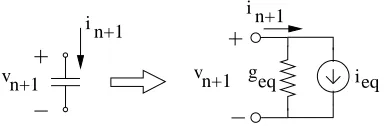
Figure 3.7 Associated Discrete Model for a Conductance . . . 49
Figure 3.8 Associated discrete model for a linear capacitor based on the BE form. . . 52
Figure 3.9 Associated discrete model for a linear inductor based on the BE form. . . 53
Figure 3.10 Discretized Oscillator model using associate discrete modeling. . . 54
Figure 3.11 Transient start up for Oscillator. . . 56
Figure 4.1 Transient start up for Oscillator, with time step 2.5 ps. . . 59
Figure 4.2 Autocorrelation for normally distributed white noise. There is an impulse of amplitude 1 at lag=0. . . 61
Figure 4.3 Autocorrelation of the oscillator output for delay,τ=100p s (time step is set to 2.5 ps). . . 62
Figure 4.4 Auto correlation of the oscillator output for zero delay,τ=0 (time step is set to 2.5 ps). . . 62
Figure 4.5 Phase noise including transient effects. The phase noise at 100 Hz offset from the carrier is 9.8 dB below the level of the carrier (Q=400, time step=2.5 ps). . . 65
Figure 4.6 Number of cycles skipped to minimize error due to transient. . . 66
Figure 4.7 Phase noise of Colpitts oscillator withQ=15 noiseless circuit elements (L= 28 nH,C1=9.3 pF andC2=1 pF ). 0 db corresponds to -9.8 dBc. . . 66
Figure 4.8 Phase noise implemented using double precision. 0 db corresponds to -9.8 dBc. 69 Figure 5.1 Phase noise of oscillator with delay 100 ps andQ=400 (L=25 nH,C1=1 pF,C2 =1.26 nF). 0 dB corresponds to -9.8 dBc. . . 72
Figure 5.2 Effect of Delay on phase noise,Q=400 (L=25 nH,C1=1 pF,C2=1.26 nF). . . . 73
Figure 5.3 Autocorrelation of the oscillator output with a delay of 200 ps (time step=2.5 ps). 73 Figure 5.4 Equivalent circuit for the oscillator loop gain with simplifying assumptions, no transistor feed-back and resistive loading across the output terminals only. . . . 74
Figure 5.5 Effect of Q on phase noise. 0 dB is considered as -9.8 dBc . . . 77
Figure 6.1 Statistical properties of white noise. Figure is taken from[15]. . . 80
Figure 6.2 Autocorrelation vs PSD of white noise. Figure is reproduced from[3]. . . 81
Figure 6.3 Simple first order low pass RC filter,R=5 KΩandC =1 pF. . . 82
Figure 6.4 Bode plot and pole-zero plot for RC filter, withR=5 KΩ,C =1 pF (implemented in Maple 18). . . 83
Figure 6.5 Baseband noise model. FIgure is taken from[48]. . . 83
Figure 6.6 Baseband discretized model. . . 84
Figure 6.7 Phase noise with addition of baseband white noise,Q=3.7, carrier-to-noise ratio=100 dB (L=30.4 nH,C1=1 pF andC2=10 pF). 0 dB is considered as −9.8 dBc. . . 85
Figure 6.8 Phase noise withQ=17.8, with and without white noise (SNR=88 dB). 0 dB is considered as−9.8 dBc. . . 87
1
INTRODUCTION
1.1
Objectives
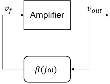
In this thesis, simulation of oscillator phase noise is reported. A simple model of an oscillator is analyzed in time and the frequency domain. The phase noise characteristics of the oscillator are calculated.
The purpose of the research described is to present a very simple model of an oscillator that presents the observed characteristics of flicker noise. The work demonstrates that flicker noise originates from a very simple process: time-delayed feedback of a weakly nonlinear system. The same process that describes chaos and long memory effects.
1.2
Motivation
noise is associated with the random motion of carriers in a material and the extent of the motion is proportional to the resistance of the material and its temperature. Shot noise is generally found in junction semiconductors, although it was originally observed in vacuum tubes, its existence is attributed to the motion of charges across a junction formed by joining two semiconductor materials with opposite charge concentrations.
The origin of flicker noise, also referred to as 1/∆f noise where∆f is the frequency offset from the carrier, is still somewhat ambiguous in the sense that there is no general agreement on its sources. Flicker noise is a more general form of power law noise or a 1/∆fαnoise whereαis considered to have discrete integer values between 0 and 5. Its various manifestations are found not just in electrical circuits but also in a wide spectrum of scientific situations which is perhaps the biggest reason for there being no unified explanation on the origins of such a noise source. Examples of flicker noise that have been observed includes vacuum tubes[52], height of the floods of the river Nile[18], self-organized criticality and sandpile slides[4], fluctuations in neuro-membranes[45], sunspot numbers in a 11 or 22 year period of the solar cycle[50]. Other examples can be found in [53].
100 Hz 1 kHz 10 kHz 100 kHz
Phase noise (dBc/Hz)
3
f −
f 0
1
f −
2
f −
∆f
0
−50
−100
−150
Figure 1.1Measured phase noise of a 50 MHz BJT varactor-based VCO[32]. Three phase noise regions are identified asf−3(having a slope of−9 dB/octave),f−2(having a slope of−6 dB/octave), andf−1(having a
slope of−3 dB/octave) Figure is taken from[32].
offset from the carrier (i.e., the average oscillation signal). For example, the phase noise spectrum of a 50 MHz BJT varactor-based VCO is shown in Figure 1.1 has regions with slopes of∆f−1,∆f−2, and∆f−3. The phase noise of oscillators and also of amplifiers have been observed to have slopes of∆f−4,∆f−5as well[55].
1.2.1 Treatment of Flicker noise is oscillators
The first substantial treatment of flicker noise in electronic oscillators was due to Leeson[35]. Leeson determined that the oscillator phase noise has a region with∆f−3dependence that is due to low-frequency∆f−1noise, a∆f−2region due to white noise in the bandwidth of the oscillator’s tank circuit, and also a white noise region outside the bandwidth of the tank circuit. He provided an important observation that increasing theQof an oscillator feedback path reduces phase noise.
The next advance that influenced and lead to improvements in oscillator design was the phase noise model introduced by Hajimiri and Lee[21]. In essence this model identified a source of flicker noise as white noise converted from harmonics of the oscillation frequency. Their time-invariant model provides a richer description of phase noise, but it does not describe∆f−1noise or∆f−n, n>3, noise that is observed with oscillators.
Various physical theories have proposed that flicker noise originates from nonlinear dynamics and chaos[10, 17, 32, 54, 61, 62]. In this model flicker noise derives from a nonlinear process with delayed feedback. In this research, we show that this is correct and we present an easily understood model of a microwave oscillator.
A common approach to the analysis of noise in oscillator circuits, and indeed to circuits with periodicity, is a perturbation analysis[36, 37]. In this analysis, a free–running oscillator described by
˙
x(t) =f(x(t)) (1.1)
wherex(t)and ˙x(t)areN–dimensional independent variables of the circuit of oscillation frequency f0, is perturbed by a small, zero-mean Gaussian noise sourcen(t)to modify the analysis equation to
˙
x(t) =f(x(t)) +B(x(t))n(t). (1.2)
the second term gives rise to phase modulation (PM) of the response. This analysis is performed by the Floquet theory of linear time-periodic differential equations, and under the restrictive conditions imposed on the nature of the noise, it can be used effectively to model the noise in a circuit simulation environment. However, if the circuit has larger levels of noise or if the noise has multiplicative effects on the state variables so as to violate the linearity condition, this method of analysis breaks down [48].
Other approaches to modeling oscillator circuits with flicker noise are based on replacing the ordinary differential equations in a circuit simulator by stochastic differential equations and using intermittency-based noise sources[32, 33], with intermittency being a characterization of chaotic behavior. A key feature of any chaotic intermittent function is that it exhibits regular laminar sections separated by intermittent bursts of seemingly random behavior and this response can be generated using a simple nonlinear iterative deterministic function. Certain intermittent chaotic functions have been used to generate sequences with long memory characteristics. These sequences have slowly decaying correlations, which is an essential property of flicker noise. When these intermittent functions are used as sources of flicker noise in circuits, the differential equations representing the circuit are now stochastic. One of the main differences between Ordinary Differential Equations (ODEs) and Stochastic Differential Equations (SDEs) is that when integrating an SDE to find a solution, the point in the interval where the integral is evaluated matters. For a random function h:[0,T]→ ℜwith intervals 0=t0<t1<t2. . .<tN =T, evaluating a integral at the starting point of each interval (the so-called Itô form), gives a different result if the evaluation occurs at the midpoint of each interval (the so-called Stratonovich form). While the interpretive nature of SDEs can seem troubling at first, it has been shown[11]that when a stochastic function involves multiplications of stochastic functions – the more general case – the Stratonovich interpretation is the correct one. Another upside of using the Stratonovich form is that conventional rules of calculus can be used to solving a system of SDEs (the Itô form requires modified calculus rules), which makes it easy to implement these ideas in a circuit simulator. While this accurately models the flicker noise observed in microwave oscillators down to very low frequencies, the complexity of the approach does not lend itself to the development of intuition.
1.3
Original Contributions
This work represents a first attempt at using quad precision to simulate phase noise in microwave oscillators. It is found that flicker noise has one of its sources lying in the dynamics of a nonlinear system with time delayed feedback. Such a system is inherently chaotic in nature and possesses long term memory effects. The dynamics of chaos are evident as a long duration autocorrelation char-acteristic. As has been experimentally observed, phase noise is affected by oscillatorQ. Baseband white noise affects the nonlinear dynamics of chaos presenting what is analogous to upconversion of baseband white noise to the oscillation frequency. The phase noise of a microwave oscillator is presented as being the result of a chaotic process.
The oscillator model developed to implement such a system is illustrated in Chapter 3. The corresponding frequency domain results clearly shows 1/∆f3and 1/∆f slopes where∆f is the frequency offset from the carrier. Varying theQof the oscillator tank circuit, causes a change in the dynamics of the nonlinear system. An increase in delay causes the phase noise level to decrease. Such an increase also causes the intermittency and hence long term memory of the system to increase. This has not been observed and analyzed by previous phase noise models. Baseband white noise changes the dynamics of the system. It leads to 1/∆f2slope in the spectrum of the oscillator.
1.4
Overview
Chapter 2 is a concise review of a large body of literature on noise in systems. The attempts of various researchers to provide physical explanations for the noise phenomenon has been explored and a brief overview on these efforts is provided. Also reviewed are the approaches to modeling noise and in particular, phase noise in oscillators.
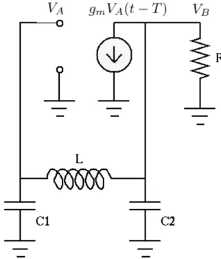
Chapter 3 introduces a simple model of a microwave Colpitts oscillator. This model is imple-mented using a nonlinear function with time delayed feedback. The oscillator is tuned to operate at 1 GHz. Its lumped element components are modeled using an associate discrete modeling technique and implemented using backward euler form. The different tools and software used to simulate are briefly reviewed.
In chapter 4, the various trade-offs implemented for simulation of phase noise are discussed. Time domain properties of the oscillator are illustrated by its autocorrelation function. Impact of the usage of quad precision over double precision for phase noise simulation is illustrated. The importance of omission of the initial transient and the corresponding effect on phase noise is presented.
factor of the oscillator is derived using the conventional definition of Q factor. Intermittency variation with delay is briefly discussed with corresponding impact on phase noise of the oscillator.
Chapter 6 adds baseband white noise to the modeled oscillator. White noise is generated using the normal distribution function in C++. This noise is passed through a first order low pass RC filter to generate baseband white noise. The effect of addition of baseband white noise on phase noise level of oscillator is discussed.
Finally Chapter 7 summarizes this work and provides guidelines to design oscillators with low phase noise.
1.5
Summary
2
LITERATURE REVIEW
2.1
Introduction
This chapter is a brief survey of the vast amount of literature available on the history of the under-standing of noise and noise processes. This chapter is by no means comprehensive but it makes an attempt to mention a fair number of references on the subject ranging from the historical origins of noise to some more recent approaches to phase noise modelling.
Section 2.2 is a brief introduction to thermal noise found in electrical circuits followed by Section 2.3 which is an introduction to shot noise. Section 2.4 surveys theories of the physical origin of flicker noise and various mathematical models to describe flicker noise processes. Section 2.5 describes phase noise in oscillators. It covers various topics ranging from importance in practical systems, negative effects due to it, various observation in practical oscillator systems. In the end it covers major literature on various models aimed to describe phase noise in electronic oscillators.
2.2
Thermal Noise
Figure 2.1Thermal noise equivalent circuits. Figure is reproduced from[31].
random voltage or current generated across the the terminals of the conductor, with resistanceR, as in Figure 2.1
The power spectral density (PSD) ofVn(t)andIn(t)are related as:
SVn(f) =R
2S
In(f). (2.1)
We can derive the Power Spectral Density (PSD) of the voltage spectrum using the principles of thermodynamics in accordance with the developments of Nyquist in 1928,[46]. This development is briefly discussed below and yields find the amount of thermal noise power in a signal. The results is dependent, to a good approximation, only on the temperatureT, and the bandwidth of the receiver.
Suppose then that the receivers bandwidth isBHz, and consider that the noisen(t)is restricted to the time interval[t1,t2]. By the sampling theorem, this signal can be represented by its samples spaced 1/(2B)seconds apart, and so the entire signal can be represented by 2B∆t samples, where ∆t =t2−t1. We can say that the noise signal has 2B∆t degrees of freedom. Now there is a theorem from statistical mechanics (Boltzmanns Law) that for any motion, for every degree of freedom, there is an average kinetic energy of12kBT joules, wherekB is the Boltzmanns constant, i.e., 1.38×10⁻²³ J/K. Thus the (average) energy in our noise signal isB∆t kBT joules and the power (energy per unit time) isB kBT watts. The bandwidthB is arbitrary, so we can divide it out and conclude that the power per unit of bandwidth iskBT watts. This value is called the power spectral density of thermal noise, and is usually denoted by the symbolN0. In summary, the power spectral density of thermal noise is
N0is sometimes called the one-sided noise spectral density, since only positive frequencies are considered.
We stated above that the average kinetic energy per degree of freedom in any motion is 12kBT, a result due to Boltzmann. But Boltzmanns law in fact gives not only the average energy of the motion, but the distribution of the energy as well. Indeed, the probability density function for the energy in a single oscillator at temperatureT is the exponential density,
p(x) = 1 kBT
e −x
kBT (2.3)
That is, the probability that the energy lies between the limitsx1andx2is
P r x1≤E ≥x2=
Z x2
x1
p(x)d x. (2.4)
It is an easy exercise in calculus to show that 2.4 implies that the average energy iskBT, i.e.,
〈E〉=
Z ∞
0
x p(x)d x=kBT (2.5)
Here the notation ’〈x〉’ indicates the ensemble average ofx. The energyE is the total energy, i.e., the sum of the potential and kinetic energies. On average they are equal, so by Equation (2.5) the average kinetic energy is 12kBT, just as we stated above.
Planck showed that the distribution of the energy is not given by the exponential density 2.3 but rather by a discrete density of a similar form. He showed thatE can assume only the discrete set of values 0,E1,2E1,3E1,..., whereE1=h f, wheref is the frequency of motion, andhis Plancks constant,h=6.62×10⁻³⁴J sec. There are two important differences from Boltzmanns density: the possible values for the energy are discrete, and the distribution is dependent on the frequency. The exact form of Plancks density function is the geometric density,
pn=P r E=n E1=αe−n E1/kBT, (2.6)
which should be compared to the Boltzmann density in Equation (2.3). The constantαin 2.6 is determined by the condition P
n≥0
pn=1, and it turns out to be,
α= (1−e−h f/kBT). (2.7)
〈E〉=X n≥0
n E1pn=kBT x
ex−1, (2.8)
wherex=h f/kBT. If we recall that〈E〉is the sum of the average kinetic energy and the average potential energy, and that the thermal noise is due to the kinetic energy of the electrons in the receiver, it follows that for every degree of freedom in the motion there is an average kinetic energy of,
1 2kBT
x
ex−1 (2.9)
Hence the power spectral density of thermal noise is,
N0=kBT
h f/k
BT eh f/kBT−1
(2.10)
which has the SI units of W/Hz.
Finally, we should add that while the power spectral density as given by Equation (2.10) tells us about the variance of thermal noise, (its mean is zero), it does not tell us more about what kind of distribution the noise has. However, since thermal noise is caused by the independent contributions of many identical particles, the central limit theorem suggests, and experiment verifies, that thermal noise is a Gaussian process[15]. Thus we may say that thermal noise is a mean-zero, gaussian random process with power spectral density given by Equation (2.10).
For a more thorough examination of thermal noise in a resistor the reader is refered to Nyquists original work[46].
With inductors and capacitors, thermal noise is mainly attributed to noise contribution from its parasitic resistances. There has been some recent advanced discussion in[19]and[41].
The power spectrum is simply related to the autocorrelation function by the Wiener - Khinchin theorem, found by taking the inverse fourier transform of the power spectrum. This suggests that regardless of the probability distribution function of the signal, a flat power spectrum will correspond to an autocorrelation of a delta function. Hence we can say that thermal noise has zero correlation with its past events, and therefore forms a memoryless system.
2.3
Shot Noise
Electrical current do not flow uniformly and does not vary smoothly in time like the standard water flow analogy. Current flow is not continuous, but results from the motion of charged particles (i.e. electrons and/or holes) which are discrete and independent. At some (supposedly small, presumed microscopic) level, currents vary in unpredictable ways. It is this unpredictable variation that is called shot noise.
The carrier entering the junction (or channel) must do so as a purely random event and indepen-dent of any other carrier crossing this point. If the carriers are not constrained in this manner then the resultant thermal noise will dominate and the Shot Noise will not be observed. A physical system where this constraint holds is a pn- ˆjunction. The passage of each carrier across the depletion region of the junction is a random event, and because of the energy barrier the carrier may travel in only one direction. Every carrier that crosses the depletion region generates a pulse. This arrival rate of pulses can be modelled by a Poisson arrival process of rateλ. The power spectral density can be derived using Van der Ziels technique discussed in[64], which is briefly discussed below.
In order to find the fluctuation, first defineN as the number of carriers passing a point in a time intervalτat a raten(t). Then
N=
Z τ
0
n(t)d t (2.11)
¯
N =n¯τ (2.12)
Where ¯N =〈N〉and ¯n=〈n〉are ensemble averages and this results follows from the fact that time averages equal ensemble averages (the Ergodic theorem). If we define a new random variable ∆N such that
∆N=N−N¯ (2.13)
Then we have removed the d.c. term leaving only the fluctuation. If we also define the random processXτthen for sufficiently largeτwe have
Xτ=∆N
τ (2.14)
Note that for a Poisson process ¯N=varN =∆N¯ 2and ¯n=varn[20], where var is the variance of the process, therefore
¯
Xτ2=∆N¯ 2 τ2 =
varN τ2 =
¯ N τ2=
¯ nτ
τ2 = varn
τ (2.15)
v a r n=τX¯τ2 (2.16)
Now applying the Wiener-Khinchin theorem yields,
Sn(0) =τlim
→∞2τ
¯
Xτ2=2varn (2.17)
To convert to current we prove Schottkys theorem. The spectral intensity of the fluctuating currentI(t)of average ¯I is
SI(0) =2qI¯ (2.18)
WhereSI(0)is the spectral density of the current fluctuations.
This derivation can be enhanced by assuming a time-varying rate for the Poisson process and that successive pulses have a degree of overlap, but in all cases it can be shown that the shot noise process has a white PSD and follows Gaussian distribution[15].
Thus, we can see that Shot noise has its autocorrelation, a delta function (similar to thermal noise). Hence, shot noise also forms a memoryless system.
2.4
Flicker Noise
Flicker noise, or 1/f, noise in electrical circuits has generally been accredited to charge trapping and detrapping in conductors or transistors. Unlike other noise sources, a widely accepted explanation of the source of 1/f noise has eluded scientists. The first spectral density measurement of 1/f noise was published by J. B. Johnson[28]. In his 1925 paper Johnson was experimentally studying Schottky0s prediction of shot noise in vacuum tubes. He found that at high frequencies the measured
noise agreed with prediction but at lower frequencies its deviation from prediction was substantial. The magnitude of this excess spectral density varied as the current squared and, although he made no comment on the frequency dependence, his published data show the excess noise to be proportional tol/f. He ascribed the effect to irregular temporal changes in the cathode emissivity. Since then this type of low-frequency noise has been observed in a variety of engineering and scientific situations and perhaps the only thing that is universally agreed upon is the ubiquity of the phenomenon. Forms of 1/f noise are observed in many of areas in[25],[59]
• Voltages or currents of:
Vacuum tubes, diodes, transistors.
carbon microphones semiconductors metallic thin-films aqueous ionic solutions
• the frequency of quartz crystal oscillators
• average seasonal temperature
• annual amount of rainfall
• rate of traffic flow
• the voltage across nerve membranes and synthetic membranes
item the rate of insulin uptake by diabetics[13]
• economic data[39]
• the loudness and pitch of music[61]
The presence of 1/f noise in such a diverse group of systems (plus others not mentioned) has led researchers to speculate that there exists some profound law of nature that applies to all nonequilibrium systems and results in 1/f noise. Numerous specific models have been proposed, but not one can account for the presence of 1/f noise in even most of the systems listed. Perhaps the only similarity among these systems is the mathematical description that leads to 1/f noise.
Many attempts has been made to understand the characteristics of 1/f noise[9]. Let us discuss some major statistical properties of 1/f noise.
2.4.0.1 Is1/f noise presence at equilibrium?
The work of many physicist and in particular that of F. N. Hooge and collaborators[24], produced several empirical formulas for 1/f noise in resistors, and in particular Hooge[23]showed that the 1/f voltage spectral density can be parametrized by the formula
Sv(f) =γ
VD C2+β Ncfα
(2.19)
2.4.0.2 Is the1/f noise process Gaussian?
There are two important reasons to answer this question: in the first place a Gaussian process is completely characterized by its average value and by the spectral density; secondly linear processes, like simple diffusion, are always Gaussian, therefore Gaussianity is an important indicator of linearity at the microscopic level.
To demostrate linearity Voss[58]proved that 1/f noise showed linearity and Gaussianity in several conductors. However, it was later demonstrated that the noise processes observed by Voss were reasonably Gaussian and did not show linearity. Later several groups reported non-Gaussian signals, but Gaussianity can always be recovered at the macroscopic level from the superposition of many microscopic processes (this is a manifestation of the central limit theorem). From the theoretical point of view linearity is not expected, since many attempts to understand 1/f noise are based on the behavior of nonlinear processes.
Notice that the properties that we have discussed in this section have been tested on conductors only, i.e. on one very special subset of the systems that display 1/f noise, therefore we cannot draw any general conclusion from these observations.
There are several mathematical models in the literature that have been proposed for modeling 1/f noise. While some of them use physical intuition to explain this phenomenon, others use a broad array of mathematical functions to produce a model for 1/f noise. Below we briefly discuss some of these models.
2.4.1 A1/fαresponse deriving from the superposition of relaxation processes
Schottky[52]developed a simple explanation of 1/fαnoise in vacuum tubes. His explanation is that a free carrier is immobilized or trapped when it falls into a recombination center (trap). When several such carriers are trapped, it means that they are not available for conduction and as a result, the resistance of the semiconductor is modulated. If in the simplest case, a single trap is considered, then the kinetics of the fluctuation are characterized by a single relaxation time or time constantτz. If this trapping process obeys a Poissonian statistic, then the correlation of this process is purely exponential and its spectrum is Lorentzian. The contribution to the vacuum tube current from the cathode surface trapping sites, which release the electrons according to a simple exponential relaxation lawN(t) =N0e−λt fort ≥0 andN(t) =0 fort <0
The Fourier transform of a single exponential relaxation process is[52]:
F(ω) =
Z ∞
−∞
N(t)e−ιωtd t=N0
Z ∞
−∞
e−λ+ιωd t = N0
therefore for a train of such pulsesN(t,tk) =N0e−λ(t−tk)fort ≥tk andN(t,tk) =0 fort <tk, we find
F(ω) =
Z ∞
−∞
N(t,tk)e−ιωtd t =N0
X
ke
ιωtk
Z∞
0
e−λ+ιωd t = N0 λ+ιω
X
ke
ιωtk (2.21)
and the spectrum is
S(ω) = lim T→∞
1 T |F(ω)|
2= N 2 0
λ2+ω2Tlim→∞ 1 T|
X
ke
ιωtk|2= N
2 0n
λ2+ω2 (2.22) where n is the average pulse rate and the triangle brackets denote an ensemble average. This spectrum is nearly flat near the origin, and after a transition region it becomes proportional to 1/ω2 at high frequency. This was sufficient for Schottky, who had found such a dependence in Johnsons data and provided a crude explanation of the frequency slopes existing in the plots. Later, he found that a single relaxation process was not enough and that there had to be a superposition of such processes, with different relaxation ratesλ[7]. Thus, using this theory three characteristic regions: a white noise region at very low frequency, a 1/f noise intermediate region and a 1/f2region at high frequency were predicted.
2.4.2 Transmission line model of1/f noise
The author in[29]introduced a simple RC transmission line model which when fed with white noise produced 1/f noise at its output. The circuit is shown in Figure 2.2.
The circuit consists of an infinitely long transmission line and fed with a white noise current source of magnitudeI at its input. The impedance of this line is
Z(f) =
v
t R
2πf C (2.23)
where R and C are the resistance and capacitance per unit length respectively. The PSD of the voltage at the output of the line is
SX(f) =I2 R
2πf C. (2.24)
Assuming a line of infinite length,SX(f)is proportional to 1/f down to zero frequency. On the other hand, if the line is of finite length, then there will exist a lower frequency below whichSX(f)is white and its value is
flow= 1
White Noise
RC line
R R R R
C C
C
Figure 2.2Lumped RC transmission line excited by a white noise current source. Figure is reproduced from[29].
with`being the length of line. Keshner went on to derive an autocorrelation function for this model and proved that it consists of a sum of two terms: a nonstationary one and a stationary one, making the overall function nonstationary. Keshner also showed that if the time of observation was much smaller than the time elapsed since the system was turned on, then this autocorrelation function could be considered almost stationary.
2.4.3 Noise in diffusion processes
Most of the early noise studies were carried out on resistors, operational amplifiers or other electronic equipment and systems. A special emphasis was placed on resistors, and thus it was quite natural to identify simple random processes like the simple random walk and more general diffusion processes as possible origins of 1/f noise. Let us start with the simple stochastic differential equation for the Wiener process
d x
d t =n(t) (2.26)
that describes Brownian motion in one space dimension, wherex(t)is the position of the Brownian particle, andn(t)is a Gaussian white noise process with standard deviationσ, so that autocorrelation ofn(t) =σ2δ(τ). The spectral density ofn(t)is justσ2/2π, and since Equation (2.26) implies the following relation between the Fourier TransformsX(ω)andN(ω)of the two processes
−ιωX(ω) =N(ω) (2.27)
We see that the spectral density ofxis
Sx= σ2
Figure 2.31D Brownian motion realization. Figure is taken from[16]
And thus we conclude that Brownian motion has a 1/f2spectrum. An example of a sample realization of a 1D brownian motion is shown in Figure 2.3. Brownian motion is considered scale invariant. Intuitively this means that a sample path realization as in Figure 2.3 looks the same in a probabilistic sense under any resolution. If the same simulation is run with a different timestep, the resulting sample path will have identical random statistical properties. These formulas show that neither Brownian motion in position space nor Brownian motion in velocity space can adequately describe 1/f noise, at least in one space dimension only the spectrum falls off too fast. In[16]it is shown that using a random driving term in the diffusion equation can lead to a 1/fαspectra.
2.5
Phase Noise
Figure 2.4Uncertainty in carrier frequency due to phase noise.
about the carrierfc.
Phase noise has many definitions of which the most widely accepted is based on single-sideband phase noise, relative to carrier. This is stated as the power realtive to the carrier in 1 Hz bandwidth at some frequency offset from the carrier. This definition will be used to quantify phase noise in all cases described here.
The instantaneous output of an oscillator can be represented by the equation
Voutput(t) =V0cos[2πfct +φn(t)] (2.29)
The functionφn(t)affects the phase of the output signal and its random nature with respect to time, gives rise to phase noise. The PSD of the oscillator can be related to the PSD of the phase noise according to:
Soutput(f) = P
2[Sφ(f +fc) +Sφ(f −fc)] (2.30) whereP is the power of the carrier. Pragmatically, the oscillator would contain amplitude noise (not modelled in the Equation (2.29) and phase noise. The amplitude noise can be added by modifying the equation above as:
Voutput(t) =V0[1+α(t)]cos[2πfct+φn(t)]. (2.31)
Figure 2.5Components of noise.
saturated or limited, the oscillator circuit rejects amplitude noise and thus phase noiseφn(t)is the relevant source of noise in oscillator circuits.
We can express Equation (2.31) in the phasor domain by the transformation
Voutput(t) =V0[1+α(t)]cos[2πfct +φn(t)] =R e[(A+α(t)]e ω0te φn(t)]. (2.32)
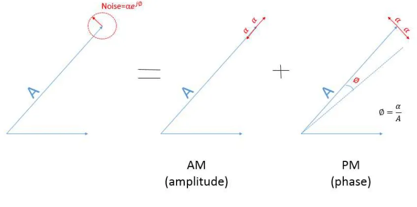
A corresponding phasor diagram is shown in Figure 2.5 where the noise is decomposed as its phase and amplitude vector components.
In Figure 2.5,Arepresents the amplitude of the desired signal rotating at an angular frequency ω0. Noise signal,αe φn is superimposed on the original signal. This noise signal has its own random amplitudeαand random phaseφn. The amplitude noise is in phase with the desired signal, whereas the phase noise is orthogonal to it. Due to limiting mechanism of the oscillator, the amplitude is going to be saturated resulting in amplitude fluctuations being rejected. A point to be made here is that the orthogonal component has a phase variation,φ≈α/A, hence we can say that the phase variation is going to be related to the amplitude fluctuations. Another insight one can gain form this is that by increasing the original amplitudeAof the desired signal the phase noise can be reduced.
of this is explained using the circuit in Figure 2.6.
Figure 2.6Varactor tuned VCO. Figure is taken from[38]
Figure 2.7Transmitter. Figure is taken from[38]
2.5.1 Importance of phase noise
It is important to study phase noise and to understand its origins so that we can predict its effect on signals, mitigate the negative effects due to it, and in the end build higher performance systems.
To understand the importance of phase noise, suppose we have a transmitter as shown in Figure 2.7(a) in which an oscillator is used to upconvert the baseband signal to the desired high frequency RF signal. If the VCO used here has large sidebands due to high phase noise, this noise gets modulated onto the baseband signal. Due to this the output would contain a spectrum in which signal components appear in adjacent channels as shown in Figure 2.7(b). This leads to adjacent channel interference. To control the level of interference stringent spectral masks have been established for transmit signals. Thus oscillator phase noise must be very low.
In the case of receivers, if we are trying to detect a small desired signal with center radian frequency,ωR F, next to a large blocker as shown in Figure 2.8(a). After passing through the mixer, the signals are down converted to an intermediate frequency using a VCO, having bad phase noise. The phase noise gets modulated onto the signals leading to masking of the desired signal, shown in Figure 2.8 (b), causing self-interference. In order to avoid this, we need to minimize the phase noise of the oscillator. One might think, that such a blocker can be removed using bandpass filters, but as these signals are extremely close to one another we would need a very high Q filter which is not realizable. Another solution might be to use a phase locked loop, to achieve some filtering within the band.
Figure 2.8Receiver interference.
elliptical shape of the smeared demodulated data shows only phase noise. If instead we had a circular smearing of demodulated data, it would correspond to amplitude noise in addition to phase noise.
Figure 2.9Constellation Diagram. Figure is taken from[1].
2.5.2 Observations of Oscillator noise in the Frequency Domain
[56]presented a discussion on the observations of phase noise. The presentation in this section follows that discussion. The most puzzling noise observed with oscillators is the noise observed at a small frequency offset from the carrier (i.e. the average oscillation signal). To develop an ap-preciation for the breadth of observations, the signals produced by several different oscillators will be considered. First, Figure 2.10 is a plot of the phase noise observed at the output of several
Figure 2.10Measured phase noise of low-frequency oscillators: (a) instrument noise floor; (b) HP 5087A frequency distribution amplifier at 5 MHz (used to drive the external reference input of several test instru-ments using a single high-quality oscillator); (c) TADD-1 frequency distribution amplifier at 10 MHz; (d) TADD-1 frequency distribution amplifier at 5 MHz; (e) Spectracom 8140T frequency distribution amplifier at 10 MHz. Five phase noise regions are identified asf−5,f−4,f−3,f−1, and white noise. The spurious
signals are related to injected harmonics of the 60 Hz power mains[56].
oscillators and amplifiers operating at 5 MHz and 10 MHz. Curve (a) is the noise floor of the noise measurement instrument and spurious tones are observed at multiples of 60 Hz, the power mains frequency. Curves (b), (c), (d), and (e) show phase noise varying in straight-line segments. Being a log-log plot, these curves show phase noise varying as f−5, f−4, f−3, f−1and f0. None of the phase noise plots here show a region with anf−2dependence, although this is observed with other oscillators[56].
accepted models are: 1) Leesons model (where, flicker noise near DC is upconverted to oscillation freqeuncy), 2) Hajmiri and Lee model ( where flicker noise away from the carrier get up converted due to nonlinearities in the oscillator loop, and 3) Unified Theory of Oscillator phase noise model (where phase noise depends only on the oscillating power, injected noise, and round-trip delay). A brief summary for these theories has been provided in next sections.
2.5.3 Leeson Model
Leeson in his paper[35]tried to explain the relationships among four commonly used spectral descriptions of oscillators short-term stability or noise behavior. He provided a heuristic derivation, presented without formal proof, the expected spectrum of a feedback oscillator in terms of the known oscillator parameters. Leeson assumed thatφ(t) in the Equation 2.29, is a zero-mean stationery random process, describing the deviations of the phase from the ideal. Leeson stated that for a feedback oscillator in which the feedback path contains an ideal resonator with a large quality factor Q, free from frequency fulctuations, the relazation time of the resonator is given by[51]:
τ=QT0
π =
2Q ω0
(2.33)
According to the oscillator equation stated above, in the case of slow fluctuations ofϕ(t), slower than the inverse of the relazation timeτ, the phaseϕ(t) can be treated as a quasi-static perturbation. The fractional frequency offset introduced by the static phaseφat a timetis
∆ω ω0
=∆f f0
= ϕ 2Qf o r
∆ω
ω
1
2Q (2.34)
This equation tells us that the oscillator would respond to the perturbation with a frequency fluctuation:
∆f(t) = f0ϕ(t)
2Q (2.35)
with associated power spectral density as:
S∆f(f) =
f
0 2Q
2
Sϕ(t) (2.36)
Thus the instantaneous output phase is:
φ(t) =2π
Z
The time-domain integration corresponds to a multiplication by 1/( ω) = 1/(2 πf)in the Fourier spectrum, thus into a multiplication by 1/(2πf)2in the spectrum. The factor 2πin above Equation (2.37) cancels with the 2πin 1/(2πf). Consequently, the oscillators slow phase fluctuation spectrum is
Sφ(f) = 1 f2
f
0 2Q
2
Sϕ(f) (2.38)
For the fast components ofϕ(t), i.e. those faster than the inverse of the relaxation timeτ, the resonator is a flywheel that steers the signal. Loosely speaking, the resonator would not respond to fast phase fluctuations; its output signal would be a pure sinusoid. Accordingly, the fluctuationϕ(t) goes through the amplifier and shows up at its output without being fed back to the input. No noise regeneration would take place in this condition, thus
ϕ(t) =φ(t) and Sϕ(t) =Sφ(t) (2.39)
By adding the effect of the fast and slow fluctuations of Equations (2.39) and (2.38), we get the Leeson formula relating the oscillators output phase spectrum to the amplifiers phase fluctuations:
Sφ(t) =
1+ 1 f2(
f0 2Q)
2S
ϕ(t). (2.40)
The above is the Leeson formula, in this formula, the noise contributed by the resonator is not considered. A typical plot for such a model is shown in Figure 2.11:
Another method for deriving the Leeson equation uses a Negative Resistance model (Figure 2.12). This model specifically shows that how white noise in the oscillator gets transformed to 20 dB/decade filtered noise at the output signal. The transistors in the oscillator is modeled as a negative resis-tance and that this transistor introduces some noisein Rn, shown in Figure 2.12. A resonator (RLC tank), shown in shunt configuration, has a positive resistanceRp(corresponding to the loss in the resonator) has a thermal noise associated with it. The active circuit and the tank resistance both inject uncorrelated noise into the tank.
In order to obtain sustained oscillations, the negative resistance of the transistor should balance out the positive resistance of the resonator. Hence, we can remove the two resistances and the circuit obtained is shown in Figure 2.13. In this equivalent circuit we would have only the noise current flowing through the LC circuit.
Figure 2.11A typical plot of the phase noise of an oscillator having low Q versus offset from the carrier. Figure is taken from[35].
Figure 2.13Equivalent circuit.
Yt a n k= ωC− 1
ωL (2.41)
Quality factor,Q=ω0C R =R/(ω0L), is introduced in the Equation (2.41), asQ can capture the slope of susceptance near resonance. Hence, Equation (2.41) becomes;
Yt a n k= Q0
R
ω
ω0 −ω0
ω
(2.42)
Let us evaluate the Equation (2.42) at an angular frequency ofω=ω0+∆ω, where∆ωis an offset from the carrier frequency. Hence,
Yt a n k= Q0
R
ω
0+∆ω
ω0 −
ω0 ω0+∆ω
(2.43)
Yt a n k=Q0 R
1+∆ω ω0
− 1 1+∆ωω
0
(2.44)
Using Taylor series we know that; 1+1x ≈1−x. Hence Equation (2.44) becomes;
Yt a n k= Q0
R
1+∆ω ω0
−
1−∆ω ω0
= Q0 R
2∆ω ω0
(2.45)
Equation (2.45) says that for very small ∆ωω
oscillation frequency.
As we are looking at uncorrelated noise sources, we would use mean square currents instead of instantaneous values to get the noise response from the tank circuit.
V02=
(in Rn
2+i n Rp
2)
|Yt a n k|2
= (in Rn
2+i n Rp
2)R2 ω0 2Q∆ω
2
(2.46)
Equation (2.46) looks like some noise multiplied by ω0
2Q∆ω
2
. We can say that the noise going in the tank is being filtered by the resonator, hence at the output we get filtered noise at around resonance. As we know the noise contributed by the resistor as opposed to the noise fro the active device. Leeson simplified the equation so as to compare the noise from active device to that from the tank. He defined this ratio, by introducingF term which is the ratio of the total phase noise injected into the tank divided by the noise coming from the finite tank resistance (this is NOT noise factor, despite the nomenclature).
F =1+in Rn
2
in Rp
2 (2.47)
The thermal noise contribution is given as
in Rp
2=4kBT R
1 2=
2kBT
R (2.48)
The factor of 1/2 appears as thermal noise from the tank is going to have amplitude and phase deviation and as we know that for an oscillator only the phase deviation remains. Thus, from the equipartition theorem one-half of the thermal noise is attributed to phase noise[34].
From Equations (2.46), (2.47) and (2.48) we get;
V02= 2kBT
R (F)R
2 ω0 2Q∆ω
2
(2.49)
The single-sideband phase noise is the sideband (phase) noise power divided by the total signal power. Here it is given as,
L(∆ω) =
V02/R Ps i g
=2F kBT Ps i g
ω
0 2Q∆ω
2
(2.50)
would go down by 30 dB/decade. This model explains both the slopes observed in phase noise of oscillators.
To summarize Leeson effect, initially it was observed that nearly every physical system has fluc-tuations that vary as 1/f at low frequencies. This includes electrical devices such as the amplifier in an oscillator feedback loop. This leads to equal amplitude phase and amplitude noise superimposed on the oscillation. Amplitude fluctuations are suppressed by the saturation of the active device so that the only noise observed in good designs is phase noise. Leeson determined that the oscillator phase noise has a region with∆f−3dependence that is due to low-frequencyf−1noise, a∆f−2 region due to white noise in the bandwidth of the oscillators tank circuit, and also a white noise region outside the bandwidth of the tank circuit. The development of Leesons oscillator phase noise model is shown in Figure 2.11. Mathematically, the single sideband phase noise is given as,[35],
L(∆f) =L(∆ω) =2F k T P0
1+
f
0 2Q∆f
2
1+ k3 ∆ω
, (2.51)
whereQis the loadedQfactor of the oscillators tank circuit andF is an empirical factor.L has the units of radians2/Hz, or in decibels,
L |dB(∆f) =10 log
2F k T P0
1+
f
0 2Q∆f
2
1+ k3 ∆f
, (2.52)
which has the units of dB/Hz or more usually as "decibels below the carrier" of powerP0, or dBc/Hz. It shows that the phase noise reduces by the square ofQ. Also there is a frequency range where the phase noise level reduces as 20 dB/decade as the carrier offset∆f increases. It also explains the effect of the power of oscillator signalP and the oscillation frequencyf0on phase noise. We can observe that for the case of a highQoscillator the term f0
2Q∆f
2
diminishes and hence the spectrum exhibits a 1/∆f slope. This explain crossover of corner frequencies such that level of 1/f2slope is reduced. We call the slope of 20 dB/decade as the region where white noise dominates. In the 1/∆f3region the slope of 30 dB/decade ia taked as indicating that low frequency flicker noise in the amplifier is being upconverted to the oscillation frequency.
2.5.4 Hajimiri and Lee Model
This theory overcomes the drawbacks of the Leeson model which made restrictive assumptions, which were applicable to only a limited class of oscillators. This model was based on a linear time invariant (LTI) system assumption and suffer from not considering the complete mechanism by which electrical noise sources, such as device noise, become phase noise. In particular, it took an empirical approach in describing the upconversion of low frequency noise sources, such as 1/f noise, into close-in phase noise. These models were also reduced-order models and therefore were incapable of making accurate predictions about phase noise in many types of oscillators.
In Leeson0s model, we combined the noise sources from the active device as well as from the resonator. In general, the noise contributed from the active devices will consist of noise from transistors, thermal noise from parasitic resistances. The transistors are switched hard from on to off and hence its noise contribution will be a function of the operating point of the transistor. This operating point is changing as the oscillator goes through its entire cycle, generating time-dependent noise in the oscillator. Likewise, we have frequency conversions of noise, i.e. noise being modulated onto the oscillation frequency from different harmonics. These contributions are not pointed out by Leesons model.
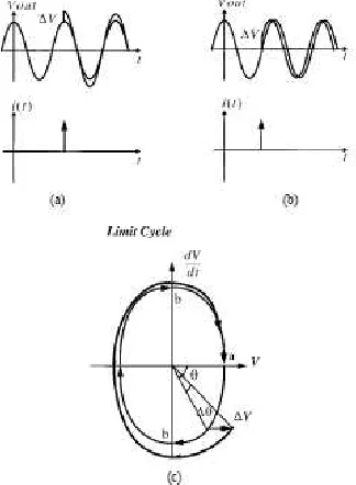
The time variant model proposed by Hajimiri and Lee in[21]is capable of proper assessment of the effects on phase noise of both stationary and even of cyclostationary noise (time-dependent noise) sources. Incorporating the time variant and cyclostationary model, Hajimiri and Lee stated that assuming the noise sources to be impulse functions, the magnitude of phase change would be dependent on the time at which the impulse is applied. If the impulse is applied when the voltage is at its peak, there will be no phase shift and only an amplitude change will result (proportional to the magnitude of the input impulse noise). However if the impulse is applied at the zero crossing, it has maximum effect on the phase and minimum on the amplitude. An impulse thus applied at a time in between will have both amplitude and phase changes. The amplitude changes can be minimized using limiters, which would cause the oscillator to follow a closed trajectory, called a limit cycle, irrespective of the starting point,[49],[43]and[14], this is illustrated in Figure 2.14. Thus only a phase fluctuation would persist indefinitely.
Figure 2.14(a)Impulse Injected at the peak, (b) Inpulse injected at zero crossing, and (c) effect of nonlin-earity on amplitude and phase of the oscillator in state-space. Figure is taken from[21].
going to be dependent on the amount of charge and capacitance of the tank. The oscillator settles after this impulse injection, but as we can see that the phase is shifted significantly. In case when impulse is injected at timet2, right at the maximum or minimum of the oscillation cycle, the voltage is increased but there is minimal change in phase (zero crossing) of the oscillator. Hence depending upon where the charge in injected, the oscillator is more or less sensitive. Intutively, the circuit is highly susceptible to variations at the zero crossovers, where the transistors are switching from on to off and undergoing a phase (state) change.
Figure 2.15Impulse injection at differnt time instants. Figure is taken from[38].
of ISF indicates where the VCO waveform is most sensitive to noise current into tank with respect to creating phase noise. We can speculate that the ISF is somewhat realted to the derivative of the output voltage (Vo u t). At the maximum or the minimum the derivative is zero (due to limit), whereas at the crossover points the derivative is maximum. Hence, ISF∝∂Vo u t/∂t. Two examples are presented to understand this, Figure 2.16, on the left a sinusoidal oscillation cycle and on the right a clipped oscillation cycle. The two ISF for both the cases is presented. Example 1 looks like a sine to cosine transformation through derivation. Example 2 has impulses only during rising or falling transitions.
In practice, the ISF is derived from the simulation of the VCO.
Suppose the impulse is injected at a timeτ, the unit impulse response for excess phase can be expressed as:
hφ(t,τ) =Γ(ω0,τ) qm a x
u(t−τ). (2.53)
Figure 2.16ISF for different VCO output waveforms. Figure is taken from[38].
at time t=τ. Thus one can calculate the excess phase noise as:
φ(t) = 1 qmax
Z t
−∞
Γ(ω0t)i(τ)dτ, (2.54)
wherei(τ)is the noise current injected in the oscillator. The ISF is periodic and is hence expanded as a Fourier series as:
Γ(2πf0τ) =pc0 2+
∞
X
n=1
(cncosn2πf0τ+θn) (2.55)
φ(t) =
c0Rt
−∞i(τ)dτ+
P∞
m=1cn
Rt
−∞i(τ)cos(nω0τ)dτ
qmax , (2.56)
wherecn are coefficients of the Fourier series. As seen above, it has got a DC component added to a number of harmonics, where the fundamental is the oscillator frequency.
The first term with thec0coefficient indicates noise that is up-converted from baseband, while the term in the summation is the contribution to the oscillator phase noise due to down-conversion of noise near the harmonic frequencies. Suppose that we inject a low frequency sinusoidal pertur-bation currenti(t)into the node of interest at a frequency of∆ωω:
i(t) =I0cos(∆ωt) (2.57)
c0. Therefore, the only significant term inφ(t) will be
φ(t) =I0c0sin(∆ωt)
2qmax∆ω (2.58)
Thus we get two impulses at±∆ωin the PSD ofφ(t).
More generally, if the applied current isi(t) =Incos[(nω0+∆ω)t], the excess phase is given as:
φ(t) =Incnsin(∆ωt) 2qm a x∆ω
(2.59)
Calculating the PSD of the output voltageSv(ω) by using linear time variant, current to phase con-vertor (discussed above), and a non linear system that represents phase modulation(PM)(transfroms phase to voltage), the injected current atnω+∆ωwould thus result in a pair of equal sidebands at ω0±∆ω, assuming these noise sourcces to be white with mean square currenti2n, then the noise spectral density is[21]:
L(∆ω) =10 log
¯
in2 ∆f
P∞
m=0cn2 4q2
max∆ω2
. (2.60)
Thus we see that, the noise at higher frequencies are down converted to the ones near the oscillation frequency. As can be seen from 2.60 and the foregoing discussion, noise components located near integer multiples of the oscillation frequency are transformed to low frequency noise sidebands for Sφ(ω) , which in turn become close-in phase noise in the spectrum ofSv(ω), this is illustrated in Figure 2.17
It can be seen that the total is given by the sum of phase noise contributions from device noise in the vicinity of the integer multiples ofω0, weighted by the coefficientscn. Thus by using the Γ(x) function and adjusting the weights ofcnwe get different slopes 1/f3,1/f2, 1/f in the PSD. In addition to the periodically time-varying nature of the system itself, another complication is that the statistical properties of some of the random noise sources in the oscillator may change with time in a periodic manner. These sources are referred to as cyclostationary. This is incorporated in this model by modifying the ISFΓ(x) by anotherΓ(eff ) function, which incorporates the cyclostationary noise sources.
![Figure 2.3 1D Brownian motion realization. Figure is taken from [16]](https://thumb-us.123doks.com/thumbv2/123dok_us/1381802.1170861/28.612.157.464.110.333/figure-d-brownian-motion-realization-figure-taken.webp)
![Figure 2.6 Varactor tuned VCO. Figure is taken from [38]](https://thumb-us.123doks.com/thumbv2/123dok_us/1381802.1170861/31.612.248.383.149.383/figure-varactor-tuned-vco-figure-taken.webp)
![Figure 2.11 A typical plot of the phase noise of an oscillator having low Q versus offset from the carrier.Figure is taken from [35].](https://thumb-us.123doks.com/thumbv2/123dok_us/1381802.1170861/37.612.140.493.421.623/figure-typical-oscillator-having-versus-offset-carrier-figure.webp)
![Figure 2.15 Impulse injection at differnt time instants. Figure is taken from [38].](https://thumb-us.123doks.com/thumbv2/123dok_us/1381802.1170861/43.612.96.541.102.351/figure-impulse-injection-differnt-time-instants-figure-taken.webp)
![Figure 2.18 Convolving in Frequency domain. Figure is taken from [38].](https://thumb-us.123doks.com/thumbv2/123dok_us/1381802.1170861/47.612.179.447.404.647/figure-convolving-frequency-domain-figure-taken.webp)