Finite Element Implementation of Advanced Constitutive Model Emphasizing on Ratcheting

(1)

18th International Conference on Structural Mechanics in Reactor Technology (SMiRT 18) Beijing, China, August 7-12, 2005 SMiRT18-B03-4

FINITE ELEMENT IMPLEMENTATION OF ADVANCED CONSTITUTIVE

MODEL EMPHASIZING ON RATCHETING

Guozheng Kang

Department of Applied Mechanics and Engineering, Southwest Jiaotong University,

Chengdu 610031, China

Phone: 86-28-87600793(o); 86-28-87601287(h) Fax: 86-28-87600797

E-mail:

;

Two visco-plastic constitutive models for simulating cyclic deformation of cyclic stable and cyclic hardening materials, respectively, were implemented into finite element code. The existed constitutive models were first extended to simulate the ratcheting and cyclic stress relaxation of the materials more reasonably by introducing a combined kinematic hardening model. In finite element implementation, new nonlinear scalar equations of implicit stress integration algorithm and new expressions of consistent tangent modulus matrix for the two discussed models were formulated by using radial return method and backward Euler integration schedule. Some numerical examples are given to verify the advantage of the implementation and the capability of the models in simulating the ratcheting, cyclic stress relaxation, and strain cyclic behavior of the materials and structure components.

Key words: Ratcheting, cyclic plasticity, constitutive model, finite element method.

1. INTRODUCTION

Ratcheting, a cyclic plastic strain accumulation, is important in designing the structure components subjected to cyclic loading, and had been studied by many researchers in last two decades for some stainless steels and ordinary carbon steels (Chaboche and Nouailhas, 1989; Ohno and Wang, 1993; McDowell, 1995; Delobelle et al, 1995; Ohno, 1997; Jiang and Sehitoglu, 1996). Recently, the capability of constitutive model to simulate uniaxial and multiaxial ratcheting has been remarkably improved, especially for the cyclically stable materials (Abdel-Karim and Ohno, 2000; Bari and Hassan, 2002; Kang et al, 2002a; b). However, the cyclic hardening feature of some materials was not taken into account reasonably, especially in the case of multi-stepped loading. It had been observed that some structure materials, such as SS304, 316 and SS316L stainless steels, exhibit significant strain-range-dependent cyclic hardening (Oyamada and Kaneko, 1993; Kang et al, 2001; 2002c), and it cannot be simply assumed that the cyclic hardening is determined by accumulated plastic strain, since a permanent stabilization of cyclic hardening will be caused, regardless of its variation with various strain ranges. Based on the Chaboche (Chaboch et al, 1979) and Ohno model (Ohno, 1982), Kang et al(2003) had constructed a new constitutive description for the strain-range-dependent cyclic hardening successfully; however, the model cannot describe the ratcheting and cyclic stress relaxation behaviours reasonably due to the choice of the Ohno-Wang nonlinear kinematic hardening model I (Ohno and wang, 1993).

To an accurate stress-strain analysis for some engineering structures subjected to cyclic loading, the implementation of advanced constitutive model into a finite element code is demanded urgently. It had been done for the rate-independent and rate-dependent plasticity, and successful simulation for inelastic deformation behaviours of some materials and structures had been obtained (Chaboche and Cailletaud, 1996; Hartmann et al, 1997; Saleeb et al, 1998; Lubarda and Benson, 2002). However, the ratcheting and cyclic stress relaxation of the material had not been discussed reasonably in aforementioned references. To solve this issue, Kobayashi and Ohno(2002) implemented a cyclic plasticity model with a general-formed kinematic hardening rule into finite element code, and obtained reasonable description for the ratcheting behaviour of some structures, where only the rate-independent plasticity was involved and the strain range dependent cyclic hardening was not discussed.

(2)

relaxation more reasonably by using a combined kinematic hardening rule similar to the Abdel-Karim-Ohno model (Abdel-Karim and Ohno, 2000). Then, the revised models are implemented into a finite element code (eg. ABAQUS(2001)) so as to describe the ratcheting and cyclic mean stress relaxation of some structures. New implicit stress integration algorithms and new expressions of consistent tangent modulus are derived for the revised models by using the radial return and backward Euler integration method. Finally, some numerical examples are given to verify the reasonability and necessity of this work.

2. CONSTITUTIVE MODELS

Since the previous model proposed by Kang et al (2002b) for cyclic stable material has a serious non-linearity caused by the high value of

m

(k)(=6), it is difficult to obtain accurate back stress integration by using the radial return method. Thus, the model is revised by using a combine kinematic hardening rule, and the revised is called as Model I hereafter. As aforementioned, the model developed by Kang et al (2003) for cyclic hardening material cannot describe the ratcheting and cyclic stress relaxation behaviours reasonably due to the choice of Ohno-Wang model I (Ohno and wang, 1993). This model is also revised to simulate the ratcheting and stress relaxation by using a combined kinematic hardening rule, and the revised one is called as Model II hereafter.

Model I. The main constitutive equations are the same as those inKang et al (2002b):

e p

_ε

ε

=

+

(1a)

σ

D

ε

e

=

−1

:

(1b)

α

s

α

s

ε

−

=

n y p

K

F

2

3

(1c)

Q

F

_y

=

1 .

5 (

s

−

α

)

:

(

s

−

α

)

−

(1d)

where

ε

,

ε

p,

ε

eand

ε

p are second-order tensors for total strain, inelastic strain, elastic strain and inelastic strain rate with respect to time, respectively;

D

is the fourth-order tensor of Hook’s elasticity. K and n are material parameters reflecting rate-dependence.

s

and

α

are second-order deviatoric stress and back stress tensors, respectively.

Q

is isotropic deformation resistance and is assumed as a constant

Q

0in Model I for cyclic stable

material. is Macauley bracket, i.e., as x≤0,

x

=

0

; as x＞0,

x

=

x

. Hereafter, bold capital letters

represent fourth-order tensors and other bold letters indicate second-order tensors. The nonlinear kinematic hardening rule is revised as

∑

=

M k

k k

r

1

) ( ) (

b

α

(2)

where, total back stress is divided into M parts denoted as

r

(k)

b

(k)(k=1, 2, …, M);

r

(k)is also assumed as a

constant

r

₀(k)in Model I. The evolution rule of

b

(k) is adopted as

⎭

⎬

⎫

⎩

⎨

⎧

₋

=

( ) ( ) ( ) )

(

3

2

p k k

k k

p

_ε

_b

b

ζ

(3)

( )

( )(

)

p

f

H

p

(k)

=

[

μ

k

+

(k)

1 −

μ

(k)

]

(4)

where,

ζ

(k)and

μ

(k)are material constants, and the critical state of dynamic recovery is reflected by a surface

0

1

2 ) ( )

(k

=

k

−

=

b

f

. Here,

b

(k)

=

(

₂3

b

(k)

:

b

(k)

)

1/2,

p

=

(

₃2

ε

p

:

ε

p

)

1/2. It is noted that

p

, rather than )

(

:

k

p

b

(3)

Model II. This model is suitable for the cyclic hardening materials, and its main constitutive equations are similar to those of Model I (Eqs. (1)), except that the isotropic deformation resistance

Q

varies with the evolution of cyclic hardening here.

The nonlinear kinematic hardening rule is also similar to Model I, except that

r

(k) is variable due to cyclic hardening and

p

f

H

p

(k)

=

μ

(k)

+

(

(k)

)

ε

In

:

b

(k)

−

μ

(k)

. (5)

In Kang et al (2003), evolution of cyclic hardening was assumed to be controlled by the same inelastic strain rate as that of back stress. However, in Model II, to avoid the evolution of cyclic hardening to be directly influenced by ratcheting factor

μ

(k), an new inelastic strain rate

p

′

(k), rather than

p

(k) is used for the evolution of cyclic hardening, i.e.,

) ( )

( )

(

:

)

(

k In k

k

f

H

p

′

=

ε

b

. (6)

Further, as an alternative description for the strain-range-dependent cyclic hardening discussed by Kang et al (2003), the cyclic hardening is decomposed as nonlinear and linear parts represented as

R

NL(k) and

)

(k

L

R

respectively, and the following evolution rules are assumed:

(

( ) ( )

)

( ) )

( )

(k NLk NLS k NLk k

NL

p

R

C

R

=

−

′

(7a)

) ( ) ( )

(k Lk k

L

p

C

R

=

′

. (7b)

Where

C

NL(k) and

C

L(k) are material constants representing the evolution rates of cyclic hardening variables.

R

NLS(k)is the saturated value of

R

NL(k). Finally,

)

)(

1 (

( ) ( ) ( )

) ( 0 )

(k k k NLk L k

R

r

=

+

−

ω

+

(8)

(

)

∑

=

+

=

M

k

k L k NL k

R

Q

1

) ( ) ( ) (

0

ω

(9)

where,

r

₀(k),

ω

(k)and

Q

₀ are material constants and can be determined by experiment.

ω

(k)is introduced to describe the Bauschinger effects of the material.

3. FINITE ELEMENT IMPLEMENTATIONS

In this section, finite element implementations of revised model I and II are elaborated on the basis of radial return method(Hartmann et al, 1997; Kobayashi and Ohno, 2002) and backward Euler integration schedule.

3.1 Discretization of Constitutive Equations

Considering the interval from step n to n+1, the backward Euler method enables us to discretize the revised constitutive models as follows:

e n p n

n+1

=

ε

+1

+

ε

+1

ε

(10)

p n p n p

n+1

=

ε

+

ε

+1

ε

Δ

(11)

)

(

:

₁ ₁

1

p n n n+

=

D

ε

+

−

ε

+

σ

(12)

1 1 1

2

3

+ +

+

=

n n

p

n

p

n

ε

Δ

(13)

1 1

1 1 1

+ +

+

₋

−

=

n n

n n n

α

s

α

s

n

(14)

1 )

1 (

1 +

+

=

n

n n y

n

t

K

F

p

Δ

(4)

n n

n

t

₊₁

=

₊₁

−

Δ

. (16)

For Model I

0 1 1 1 1 ) 1

(

1 .

5 (

)

:

(

)

Q

F

yn+

=

s

n+

−

α

n+

s

n+

−

α

n+

−

(17)

∑

= + +

=

M k k n k n

r

1 ) ( 1 ) ( 0 1

b

α

(18)

) ( 1 ) ( 1 ) ( 1 ) ( 3 2 ) ( ) ( 1 k n k n k p n k k n k

n+

=

b

+

ε

+

−

p

+

b

+

b

ζ

Δ

ζ

Δ

(19)

but for Model II

1 1 1 1 1 ) 1

(n+

=

1 .

5 (

n+

−

n+

)

:

(

n+

−

n+

)

−

n+

y

Q

F

s

α

s

α

(20)

∑

= + + +

=

M k k n k n n

r

1 ) ( 1 ) ( 1 1

b

α

(21)

(

)

exp[

(1)

]

) ( ) ( ) ( ) ( ) ( 1 k n k NL k NL n k NLS k NLS k NL

n

R

C

p

R

₊

=

−

Δ

′

₊ (22)

) ( 1 ) ( ) ( ) ( 1 k n k L k L n k L

n

R

C

p

R

₊

=

+

Δ

′

₊ (23)

)

)(

1 (

(1)

) ( 1 ) ( ) ( 0 ) ( 1 k L n k NL n k k k

n

r

R

r

₊

=

+

−

ω

₊

+

₊ (24)

(

)

∑

= + + +

=

+

M k k L n k NL n k

n

Q

R

Q

1 ) ( 1 ) ( 1 ) ( 0

1

ω

. (25)

3.2 Implicit Stress Integration Algorithm

The variables at time

t

_n(i.e. step n) are assumed to be known, and

Δ

ε

_n₊₁and

Δ

t

_n₊₁are given, then find

1

+ n

σ

that satisfies the discretized constitutive equations. In this paper, a method of elastic predictor and plastic corrector is used.

The elastic predictor can be obtained by taking the total strain increment

Δ

ε

n+1 as elastic strain, i.e.,

)

(

:

₁ * 1 p n n

n

D

ε

σ

₊

=

₊

−

(26)

Judging whether a yielding is caused according to

1 * 1 * 1 2 3 * ) 1

(n+

=

(

n+

−

n

)

:

(

n+

−

n

)

−

n+

y

Q

F

s

α

s

α

, (27)

where,

s

σ

* ₃1

(

σ

* ₁

)

I

1

*

1 + +

+

=

n

−

n

tr

. If

0

* ) 1

(n+

≤

y

F

, it implies that yielding does not occur and then

σ

*_n₊₁ is

accepted as

σ

_n₊₁. For Model I,

Q

_n₊₁

=

Q

₀; for Model II, it is given by Eq. (25). If

F

_y*₍_n₊₁₎

>

0

,

σ

*_n₊₁ cannot be

accepted as

σ

n+1 due to the yielding, and

σ

n+1can be calculated by

p n n n 1 * 1

1 +

:

+

=

σ

−

D

Δ

ε

σ

, (28)

where,

D

:

Δ

ε

np+1 is a plastic corrector. It is seen from Eq. (28) that

σ

n+1 can be readily obtained if

p n+1

ε

Δ

is

found. It had been demonstrated that this issue can be reduced to solving a non-linear scalar equation even for rate-dependent plasticity (Hartmann et al, 1997). Therefore, we will take effort to seek the equations suitable for the proposed models in the following paragraphs.

Since Model I can be taken as a simplified version of Model II regardless of the cyclic hardening, the following derivation is mainly done according to model II. Formulae suitable for model I are denoted as special ones, if necessary. Following the same steps as in Kobayashi and Ohno (2002), a new non-linear equation about

1

+

(5)

0

3

1 1 ₁

1 ) ( ) ( 1 ) ( 1 * 1 1

=

−

⎟

⎠

⎞

⎜

⎝

⎛

₊

+

−

+ + ₊ = + + +

+

∑

n

n n n M k k k n k n n n

t

K

Q

Y

r

G

Y

θ

ζ

Δ

(29)

where both

Y

_n₊₁

=

₂3

s

_n₊₁

−

α

_n₊₁ and

∑

= + + + +

=

−

M k k n k n k n n n

r

Y

1 ) ( ) ( 1 ) ( 1 * 1 2 3 *

1

s

θ

b

, as well as

) (

1

k n

r

₊ ,

θ

_n(k₊₁)and

Q

_n₊₁

are functions of

Δ

p

_n₊₁.

r

_n(₊k₁)and

Q

_n₊₁ are calculated by Eqs. (24) and (25) with the help of

) ( ) *( 1 ) ( # 1 ) (

1

(

)(

1 )

/

k k n k n k

n

H

f

b

p

ζ

Δ

′

₊

=

₊ ₊

−

(30)

Further,

( )

(

( )

)

1 1 ) ( * 1 ) ( # 1 ) ( 1 ) ( 1 k n k n k n k n k

n

c

H

f

b

c

+

− + + +

+

=

+

−

θ

(31)

)

1 (

1

1 ) ( ) ( ) ( 1 + +

=

₊

n k k k n

p

c

Δ

ζ

μ

(32)

and #(1)2

1

) ( #

1

=

+

−

+ n k k

n

b

f

,

(

#(1)

)

1/2

) ( # 1 2 3 ) ( # 1

:

k n k n k n

b

₊

=

b

₊

b

₊ , *(1) ) ( 1 ) ( # 1 k n k n k

n+

=

c

+

b

+

b

. #(1)

k n+

b

is a tentative result of ( )1

k n+

b

by

neglecting the critical state

f

(k)

=

0

and using the radial return method. If it locates onto the critical surfaces or inside, i.e.,

f

_n#₊(₁k)

≤

0

,

b

#_n(₊k₁) is accepted as

b

_n(k₊)₁; otherwise,

b

#_n(₊k₁) is radially projected onto the critical surface.

In n k k n k n 1 ) ( 3 2 ) ( ) *( 1 +

+

=

b

+

ε

b

ζ

Δ

is a predictor for each ( )1

k n+

b

, and *(1)

) ( 1 ) ( 1 k n k n k

n+

=

+

b

+

b

θ

.

The non-linear scalar equation for Model I can be obtained from Eq. (29) by setting

r

_n(₊k₁)

=

r

₀(k)and

0

1

Q

_n₊

=

. Eq. (29) can be solved by combining successive substitution method with Newton-Raphson method. The convergence of successive substitution method had been proved by Kobayashi and Ohno (2002).

3.3 Consistent Tangent Modulus

Also, the following derivation is mainly done with respect to Model II. Formulae suitable for Model I are denoted as special ones, if necessary. It is deduced by differentiating that:

)

d

(

:

d

₁ ₁ p₁

n n

n+

=

Δ

+

−

Δ

+

Δ

σ

D

ε

(33)

)

d

(

d

₂3 ₁ ₁ ₁ ₁

1 + + + +

+

=

Δ

+

Δ

n n n n

p

n

p

n

p

n

ε

(34)

)

d

(

:

d

n

_n₊₁

=

J

_n₊₁

Δ

s

_n₊₁

−

Δ

α

_n₊₁ (35)

where

1 (

1 1

)

1 1

1 + +

+ +

+

=

₋

−

n

⊗

n

n n

n

I

n

α

s

J

, (36)

⊗

represents tensor product, (:) stands for tensor contraction; and

I

is fourth-order unit tensor. Differentiating Eqs. (15) and (20) yields

) 1 ( 1 ) 1 ( 1

d

₊ − + +

Δ

=

Δ

_y_n

n n y n

F

K

F

K

t

n

p

(37)

1 1 1 1 2 3 ) 1

(

:

(

d

)

d

F

_y_n₊

=

n

_n₊

Δ

s

_n₊

−

Δ

α

_n₊

−

Q

_n₊ . (38)

If

d

Δ

s

_n₊₁,

d

Δ

α

_n₊₁ and

d

Q

_n₊₁ can be expressed in terms of

d

Δ

ε

_n₊₁ and

d

Δ

ε

_np₊₁, the consistent tangent modulus can be easily obtained from Eq. (33). For Model I,

d

Q

_n₊₁

=

0

.

(6)

d n n n

n

G

L

J

I

D

ε

σ

:

)

:

(

4 d

d

0 1 1 1 2 1 1 + − + + +

₌

₋

Δ

(39)

where,

:

(

2 )

₂3

(

0 ₁ 0 ₁

)

1 ) ( 1 0 1

1 + +

= + +

+

=

+

∑

+

n

⊗

n

M

k k n n

n

I

J

G

I

H

A

b

n

L

(40)

(

)

[

]

{

}

I

b

H

) ( ) ( 1 ) ( 1 3 2 ) ( 1 ) ( 1 ) ( # 1 ) ( ) ( 1 ) ( 1 ) ( ) ( 1 ) ( ) ( ) ( ) (

1

(

1 )

(

)

k k n k n k n k n k n k k n k n k L k NL n k NLS k NL k k n

r

f

H

r

C

R

C

ζ

θ

ζ

θ

ω

+ + + + + + + + +

+

⊗

−

+

−

=

(41) 1 1 2 3 1 0 1 2 3 0

1

(

+ +

)

+ +

+

=

n

⊗

n

+

Δ

n n

n

A

n

p

J

(42)

)

:

(

₁ ₁ ₁ ₁

0

1 + + + +

+

=

n

+

Δ

n n

′

n

p

J

b

n

(43)

[

]

( )

{

}

∑

= + + + +

=

−

+

M k k n k n k L k NL n k NLS k NL k

n

C

R

C

H

f

1 ) ( 1 ) ( # 1 ) ( ) ( 1 ) ( ) ( ) ( 0

1

(

)

b

ω

(44)

( )

[

]

{

}

∑

= + + + + +

=

−

′

M k k n k k k n k n k n

n

H

f

r

1 ) ( 1 ) ( ) ( ) ( 1 ) ( 1 ) ( # 1

1

1 b

b

θ

ζ

μ

(45)

)

:

(

1

₂3 ₁ ₁

1 ) 1 ( 1 1 ) 1 ( 1 + + − + + − + +

′

+

=

n n n n y n n n y n

K

F

K

t

n

K

F

K

t

n

A

b

n

Δ

(46)

and

_I

=

(

_I

−

1₃

₁

⊗

₁

)

d is a deviatoric operator of tensor,

1

is a second-order unit tensor.

For Model I, there are

b

0_n₊₁

=

0

, ( ) ( )

(

2₃

(

#(₁)

)

( ₁) ( ₁)

)

1 ) ( 0 ) ( 1 k n k n k n k k n k k

n+

=

r

+

I

−

H

f

+

b

+

⊗

b

+

H

θ

ζ

,

r

_n(₊k₁)

=

r

₀(k)and

the others are the same as those of Model II.

4. NUMERICAL EXAMPLES

The models have been coded as UMAT user material subroutine of ABAQUS. In numerical calculation, we use Aitken’s ∆2

process to accelerate the convergence of successive substitution, as did by Kobayashi and Ohno (2002). The material parameters are the same as those obtained by Kang et al (2002b; 2003), except for

)

(k

μ

=

.

4.1 Uniaxial Tension

The uniaxial tensile stress-strain curves of U71Mn rail steel (Model I) and SS304 stainless steel (Model II) were calculated by finite element code ABAQUS with employing a 3D 8-noded isoparametric brick element at the strain rate of 0.2%s-1. The experimental and calculated results are shown in Fig. 1. It can be seen that the calculated results for

μ

=

0 .

0

and

μ

=

0 .

15

(

μ

=

0 .

1

for SS304 stainless steel) are in good agreement with the experimental results, and the variation of

μ

has little effect on the uniaxial tensile behaviour if

μ

<

0 .

5

. As

0 .

1 =

μ

(Armstrong-Frederick model (Armstrong and Frederick, 1966) is reduced to), the simulated results have great difference from the experimental. From the calculated results shown in Figs. 2, it is concluded that as

15 .

0 =

μ

(

μ

=

0 .

1

for SS304), almost the same results for strain increment

Δ

ε

=

0 .

1 %

and

%

5 .

2 =

ε

(7)

0 1 2 3 4 5 0

200 400 600 800 1000

(a)

Experimental ABAQUS μ =0.00 ABAQUS μ =0.15 ABAQUS μ =0.50 ABAQUS μ =1.00

A

x

ia

l st

ress

σ

, M

P

a

Axial strain ε , %

0.0 0.5 1.0 1.5 2.0 0

50 100 150 200 250 300 350

(b)

Experiments ABAQUS μ =0.0 ABAQUS μ =0.1 ABAQUS μ =0.5 ABAQUS μ =1.0

A

x

ia

l

S

tr

e

s

,

M

P

a

Axial Strain , %

Fig. 1 Uniaxial tensile stress-strain curves obtained by experiment and ABAQUS: (a) U71Mn; (b) SS304.

0 1 2 3 4 5 6 0

200 400 600 800 1000

(a)

Δε =0.1%, μ =0.15 Δε =2.5%, μ =0.15 Δε =0.1%, μ =1.0 Δε =2.5%, μ =1.0

A

x

ia

l st

ress

σ

, M

P

a

Axial strain ε , %

0.0 0.5 1.0 1.5 2.0 2.5 0

50 100 150 200 250 300 350

(b)

Δε =0.04%, μ =0.1 Δε =0.10%, μ =0.1 Δε =1.00%, μ =1.0 Δε =1.00%, μ =1.0

A

x

ia

l S

tr

e

s

σ

,

M

P

a

Axial Strain ε , %

Fig. 2 Uniaxial tensile stress-strain curves with various strain increments: (a) U71Mn; (b) SS304.

4.2 Uniaxial Strain Cycling

Uniaxial strain cycling behaviour of SS304 stainless steel was calculated by employing a 3D 8-noded isoparametric brick element at

μ

=

0 .

0

. The applied strain amplitude is 2% and the strain rate is 0.2%s-1. The experimental and calculated results are shown in Fig. 3, where N represents cyclic number. It can be seen that the calculated results are in good agreement with the experimental and the non-saturation feature of cyclic hardening is also described.

-2 -1 0 1 2 3 4

-800 -600 -400 -200 0 200 400 600 800

μ =0.0 N=30, ABAQUS

N=1, E N=5, E N=10, E N=30, E ABAQUS

Axia

l St

res

s

,

MPa

Axial Strain , %

Fig. 3 Stress-strain curves of SS304 for uniaxial Fig. 4 Finite element mesh of notched-bar. strain cycling.

4.3 Uniaxial Ratcheting of Notched-bar

(8)

MPa

400

max

=

appl

σ

,

σ

applmin

=

−

200 MPa

; for SS304,

200 MPa

max

=

appl

σ

,

σ

applmin

=

−

100 MPa

; stress rate is

50MPa/s and cyclic number is 10.

0.0 0.5 1.0 1.5 2.0 2.5 3.0 -800

-600 -400 -200 0 200 400 600 800 1000

(a) μ =0.15

N=12

N=3

A

x

ia

l st

ress

σ

, M

P

a

Axial strain ε , %

0.0 0.5 1.0 1.5 2.0 2.5 3.0 -800

-600 -400 -200 0 200 400 600 800 1000

(b) μ =1.0

N=12

N=3

A

x

ia

l st

ress

σ

, M

P

a

Axial strain ε , %

0.0 0.2 0.4 0.6 0.8 1.0 1.2 -400

-300 -200 -100 0 100 200 300 400 500

(c) μ =0.10

N=3

N=12

A

xi

a

l

st

re

ss

,

M

P

a

Axial strain , %

0.0 0.2 0.4 0.6 0.8 1.0 1.2 -400

-300 -200 -100 0 100 200 300 400 500

(d) μ =0.5

N=3

N=12

A

xi

a

l

st

re

ss

,

M

P

a

Axial strain , %

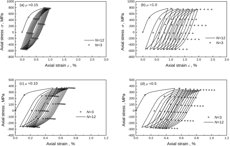
Fig. 5 Stress-strain curves of notched-bar under stress cycling near the notch-tip: (a), (b) U71Mn; (c), (d) SS304.

It is seen that for U71Mn rail steel (in Figs. 5a and 5b), as

μ

=

0 .

15

, the variation of sub-step number N in each half-cycle has almost no effect on the calculated ratcheting; when the parameter

μ

is high (such as

0 .

1 =

μ

), the calculated result for

N

=

3

has great deviation from that for

N

=

12

. It implies that if the parameter

μ

is small enough (such as

μ

=

0 .

15

), the calculation for the ratcheting of structure component can be achieved by taking fewer sub-steps (even one sub-step) for rate-dependent plasticity when the cyclic hardening is neglected. However, for SS304 stainless steel, the results (in Figs. 5c and 5d) show that even the parameter

μ

is nearly zero, accurate simulation for the ratcheting can be only achieved by using more sub-steps, this difference is caused by the introduction of

r

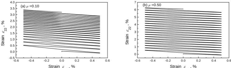
(k)and Q which are variable with the evolution of cyclic hardening.

4.4 Multiaxial Ratcheting and Uniaxial Cyclic Mean Stress Relaxation

(9)

-0.6 -0.4 -0.2 0.0 0.2 0.4 0.6 -0.5

0.0 0.5 1.0 1.5 2.0 2.5 3.0 3.5 4.0

(a) μ =0.10

St

ra

in

ε 22

, %

Strain ε 11 , %

-0.6 -0.4 -0.2 0.0 0.2 0.4 0.6 0

1 2 3 4 5 6 7

(b) μ =0.50

St

ra

in

ε 22

, %

Strain ε 11 , %

Fig. 6 Strain responses for multiaxial cyclic stressing: (a) μ=0.1; (b); μ=0.5.

0 5 10 15 20 25 30 35

0 2 4 6 8 10 12

μ =0.1

μ =0.5

M

e

an

S

tr

e

ss ,

M

P

a

Cyclic Number N , cycle

Fig. 7 Results of mean stress relaxation. Fig. 8 Shape of loading path for multiaxial cyclic stressing

5. CONCLUSIONS

In this paper, the models developed by Kang et al (2002b; 2003) were revised to simulate ratcheting and cyclic mean stress relaxation by using a combined kinematic hardening rule, and then were implemented into finite element code. The critical state of the combined kinematic hardening model enables us to obtain accurate integration for back stress efficiently by the radial return method. In the numerical implementation, a new implicit stress integration algorithm and a new expression of consistent tangent modulus are established for revised Model I and Model II, respectively. The numerical results show that an accurate simulation for monotonic tension and uniaxial strain cycling can be achieved by using a large strain increment with small

μ

, even rate-dependent plasticity is taken into account. However, under stress-controlled loading, for Model II, accurate simulation just can be achieved by setting stress increment small enough. Moreover, uniaxial/multiaxial ratcheting and uniaxial cyclic mean stress relaxation of structure component can be simulated reasonably by the extended models and their implementations in ABAQUS. Since the integration algorithm is similar to that of Kobayashi and Ohno (2002), the stability and accuracy of the algorithm are the same as those of Kobayashi and Ohno (2002), and are not discussed in details here. Moreover, since the experimental results of discussed ratcheting and mean stress relaxation for notched-bar and SS304 stainless steel under multiaxial loading path shown in Fig.8 are under-progressed now, the corresponding calculated results cannot be compared with the experimental ones.

Acknowledgements The author is grateful to National Natural Science Foundation of China (Contract No.10402037) and Theoretical Research Fund of Southwest Jiaotong University (Contract No. 2003XJB15) for their financial supports.

REFERENCES

ABAQUS/Standards User’s Manual, Version 6.2. Hibbitt, Karlsson and Sorensen, Inc., 2001.

Abdel-Karim, M., Ohno, N., 2000. Kinematic hardening model suitable for ratcheting with steady-state, Int. J. Plast., 16, 225.

Armstrong, P.J., Frederick, C.O., 1966. A mathematical representation of the multiaxial Bauschinger effect. CEGB Report RD/B/N731, Berkely Nuclear Laboratories, Berkely, UK

-0.6 -0.4 -0.2 0.0 0.2 0.4 0.6 0

100 200 300 400 500

Stre

s

σ 22

, MPa

Strain ε

11 , %

m

2

σ

a

2

σ

a

(10)

Bari, S. and Hassan, T. 2002. An advancement in cyclic plasticity modeling for multiaxial ratcheting simulation, Int. J. Plast., 18, 873

Chaboche, J.L., Dang Van, K. and Cordier, G., 1979. Modelization of strain memory effect on the cyclic hardening of SS316 stainless steel. Transactions of the 5th international conference on structural mechanics in reactor technology, Vol.L, North-Holland, Paper No. L11/3.

Chaboche, J.L., Nouailhas, D., 1989. Constitutive modeling of ratcheting effects: Part I, Experimental facts and properties of classical models. ASME J. Eng. Mater. Technol., 111(4), 384

Chaboche, J.L., Cailletaud, G., 1996. Integration methods for complex plastic constitutive equations, Comp. Meth. Appl. Mech. Engng., 133, 125.

Delobelle, P., Robinet, P., Bocher, L., 1995. Experimental study and phenomenological modelization of ratchet under uniaxial and biaxial loading on an austenitic stainless steel. Int. J. Plasticity, 11(4), 295

Hartmann, S., Luhrs, G., Haupt, P., 1997. An efficient stress algorithm with applications in viscoplasticity and plasticity, Int. J. Numer. Meth. Engng., 40, 991.

Jiang, Y., Sehitoglu, H., 1996. Modeling of cyclic ratcheting plasticity. ASME J. Appl. Mech., 63(3), 720 Kang, G.Z., Gao, Q., Cai, L.X., Yang, X.J., Sun, Y.F., 2001. An experimental study on uniaxial and multiaxial

strain cyclic characteristics and ratcheting of 316L stainless steel, J. Mater. Sci. Technol., 17(2), 219. Kang, G.Z., Gao, Q., Yang, X.J., 2002a. A visco-plastic constitutive model incorporated with cyclic hardening for

uniaxial/multiaxial ratcheting of SS304 stainless steel at room temperature, Mech. Mater., 34, 521.

Kang, G.Z., Gao, Q., 2002b. Uniaxial and non-proportionally multiaxial ratcheting of U71Mn rail steel: Experiments and simulations, Mech. Mater., 34, 809.

Kang, G.Z., Gao, Q., Cai, L.X., Sun, Y.F., 2002c. Experimental study on uniaxial and nonproportionally multiaxial ratcheting of SS304 stainless at room and high temperatures, Nucl. Eng. Des., 216, 13.

Kang, G.Z., Ohno, N., Nebu, A., 2003. Constitutive modeling of strain-range-dependent cyclic hardening, Int. J. Plast., 19, 1801.

Kobayashi, M., Ohno, N., 2002. Implementation of cyclic plasticity models based on a general form of kinematic hardening, Int. J. Numer. Meth. Engng., 53, 2217.

Lubarda, V.A., Benson, D.J., 2002. On the numerical algorithm for isotropic-kinematic hardening with the Armstrong-Frederick evolution of the back stress, Comp. Meth. Appl. Mech. Engng., 191, 3583.

McDowell, D. L., 1995. Stress state dependence of cyclic ratcheting behavior of two rail steels, Int. J. Plast., 11, 397.

Ohno, N., 1982. A constitutive model of cyclic plasticity with a nonhardening strain region, J. Appl. Mech., 49, 721.

Ohno, N., 1997. Recent progress in constitutive modeling for ratcheting, Mater. Sci. Res. Int., 3(1), 1.

Ohno, N., Wang, J.D., 1993. Kinematic hardening rules with critical state of dynamic recovery, Int. J. Plast., 9, 375.

Oyamada, T., Kaneko, K., 1993. Influence of prestraining and deformation rate on viscoplasticity and strain ageing of metal materials (the case of SCM435 steel and SUS316 stainless steel under uniaxial loading), Trans. JSME(A), 59 , 2612-2617.

Finite Element Implementation of Advanced Constitutive Model Emphasizing on Ratcheting