||||||||||||||||||||||||||||||||||||||||||||||||||||||||||||||||||||||||||||||||||||||||||||||||||||||||||||||||||||||||||||||||||||||||||||||||||||||||||||||||||||||||||||||||||||||||||||||||||||||||||||||||||||||||||||||||||||||||||||||||||||||||||||||||||||||||||||||||||||||||||||||||||||||||||||
[
**]
Electromagnetic Interrogation Using Stochastic
Inverse Problems
H.T.
Banks
* and Fumio
Kojima
†||||||||||||||||||||||||||||||||||||||||||||||||||||||||||||||||||||||||||||||||||||||||||||||||||||||||||||||||||||||||||||||||||||||||||||||||||||||||||||||||||||||||||||||||||||||||||||||||||||||||||||||||||||||||||||||||||||||||||||||||||||||||||||||||||||||||||||||||||||||||||||||||||||||||||||
1.
Introduction
The literature addressing electromagnetic imaging is recently extensive applying advanced sensor tech-nologies. This is of considerable interest in the realm of signal detection and the identification related to the development of new ceramic materials, the early detection of anomalies in polymer, metabolic func-tioning of human bodies, etc [1]. Specifically, mea-surements for reflectance of microwave tests can be employed in the evaluation of the structural integrity of composite dielectric materials. This article is fo-cused on the identification and parameter estimation of complex materials such as ceramic matrix compos-ites (CMCs) for their use in a wide range of applica-tions, such as use in components of high temperature engines [2][3]. Such composite materials would vary with uncertainly across the population of materials. Even if one begins with a deterministic model and has no initial interest in uncertainty or stochasticity, as soon as one employs experimental data in the in-vestigation, one is led to uncertainty that should not be ignored. Hence the coefficients in the mathemat-ical model are randomly varying or the model itself is led to the stochastic system. Moreover, in inverse or parameter estimation problems, an important but practical question is how successful the mathematical model is in describing the physical phenomena rep-resented by the measurement data. In general, it is very unlikely that the residual sum of squares (RSS) in the least-squares formulation is zero. Due to mea-surement noise as well as modeling error, there may not be a ”true” set of parameters so that the mathe-matical model cannot provide an exact fit to the mea-surement data. To overcome this issue, the theory of probability and statistics is an essential mathemati-cal tool in the formulation of inverse problems in the study of uncertainty propagation in dynamical sys-tems.
In this article, we summarize two alternative ap-proaches to solve our inverse problems, One possi-ble method is to consider parameter estimation of a model which can be described by stochastic sig-nal response model through noisy data collections. We summarize the computational framework with the
∗ North Carolina State University † Kobe University
Key Words: identification, parameter estimation, proba-bility, modeling, electro-magnetics, non-desructive evalu-ation.
background knowledge of the Prohorov Metric Frame-work (PMF) developed by the first author’s group in the past two decades for nonparametric estimation of probability measures using RSS [4] –[9]. Another class of methods involve Markov Chain Monte Carlo (MCMC) methods which covers a wide range of statis-tical modeling. It has also taken about two decades to penetrate mainstream of statistical practice. It pro-vides a unifying framework within which numerous practical problems can be solved (e. g. [10][11]). Most applications of MCMC to date are directed towards Bayesian inference. Therefore it is natural way to ap-ply MCMC to various kinds of inverse problems since observations and parameters of a statistical model are considered as random quantities. There have been previous efforts on parameter estimation related to
the statistical inversions using MCMC [12][13]. In
this article, we summarize an MCMC method which applies to the problems considered here [14].
2.
Classical Inverse Methodology
The Lorentz oscillator model is derived by assum-ing that an electron bound to the nucleus of an atom obeys Hooke’s law, where the displacement of the electrons from equilibrium is a result of an applied electromagnetic field. Combining the Lorentz oscilla-tor model with the Lorentz model for electronic polar-ization results in the Lorentz model for the complex relative permittivity with a single-resonance given by
b
ϵr(ω) =ϵ∞−
ωp2
ω2−iω/τ
f−ω20
. (1)
In the above equation, ϵ∞ denotes the relative
per-mittivity of the medium at infinite frequency, τf is
the relaxation time, i=√−1 is the imaginary unit,
and ωp=ω0
√
ϵs−ϵ∞ is called the plasma frequency
of the medium, where ω0 is the resonance frequency,
and ϵs is the relative permittivity of the medium at
zero frequency. Practically, it is typical for the data
to be collected as a function of the wavenumber k,
rather than frequency. Using the relationk=ω/(2πc)
where c is the speed of light, we obtain the relative
permittivity as a function of wavenumber
b
ϵr(k) =ϵ∞−
k2
p
k2−ik/τ
k−k20
, (2)
wherekp=k0
√
ϵs−ϵ∞,k0=ω0/(2πc), andτk= 2πcτf.
We will refer tok0 as the resonance wavenumber and
when it is clear that we are referring to the relax-ation time for the permittivity in terms of wavenum-ber. Thus the wavenumber model includes a set of parameter vectors
θ= (ϵs, ϵ∞, τk)t ∈ Θ⊂R3, (3)
with which one is seeking to fit values for the
mea-surement data with respect to the compact setΘ. For
simplicity, we assume that a monochromatic uniform
wave of wavenumberkis normally incident on a plane
interface between free space and a dielectric medium. In addition, we assume that the electrical field is po-larized perpendicular to the plane of incidence. With these assumptions, the fully complex reflection coef-ficient is given by
r(k;θ) =1−
√ b ϵr(k;θ)
1 +√bϵr(k;θ)
. (4)
The derivation of the reflection coefficient can be found in many electromagnetic treatments. The ob-servable information can be taken as two types of data. In the case that the observed part of the sys-tem is only reflectance (4), the signal response can be given by
h(k;θ) =|r(k;θ)|2. (5)
Traditionally, classical inverse methodologies have been focused into mathematical, statistical and com-putational aspects of inverse or parameter estima-tion problems for deterministic models with appropri-ate corresponding data noise assumptions of constant variance and non-constant variance (e.g., relative er-ror). We consider a statistical observation model of the form
Yj=h(kj;θ0) +Vj, j= 0,1,2,···,n, (6)
where θ0 denotes “true” parameters at the
mea-surement (sweeping) wavenumberkj, Vj denotes the
measurement error corresponding to the
wavenum-ber kj, and (n+ 1) is the total number of
obser-vations.Without loss of generality, we assume that
Vj,j= 0,1,···,n are independent and normally
dis-tributed with zero mean and constant covariance
ma-trixσ2
e∗In whereInis ann-dimensional identity
ma-trix. In the past several decades, one of the traditional parameter estimation problem is to seek a solution
b
θn= argmin
θ∈Θ n
∑
j=0
h(k;θ)−yjd2 (7)
where yd
j is a realization of Yj. Once we find the
minimum solution θbn of Eq. (7), the corresponding
residual error is calculated by
b
σe=
n
∑
j=0
h(k;bθn)−ydj
2
. (8)
As a result, we can evaluate the efficiency of the es-timator using the so-called “Fisher’s information ma-trix” [7].
3.
Inverse Analysis using the PMF
In a homogeneous medium, one might assume that
the resonance wavenumbersk0or the relaxation times
τ would be the same throughout the material
par-ticles. However, for composite materials, it would
vary across the population of material particles, thus requiring some type of distribution on these reso-nance wavenumbers or relaxation times in order to characterize the heterogeneous population of
parti-cles. To allow for a distributionGof either resonance
wavenumbers or relaxation times, over an admissible
set K ⊂ R, we generalize the stochastic relative
per-mittivity for the Lorenz model (2) to be
b
ϵr(k;G,θ) =ϵ∞−
∫
K
kp2
k2−ik/τ
k−k02
dG, (9)
whereG∈P(K), the set of admissible probability
mea-sures on K. The observation model is then
repre-sented by
Yj=h(kj;G0,θ0) +Vj, j= 0,1,2,···,n. (10)
In the above equation Yj is a random variable which
is composed of the reflectance with G0 the ‘’true”
probability measure andθ0the ‘’true” parameter
vec-tor at sampling wave number kj, and the statistical
properties of measurement errors Vj are assumed to
be the same as in the previous section. With the
assumptions we have made for the measurement
er-rors in the statistical model, the estimators{G,θ}t=
{G, ϵs, ϵ∞, τ}t can be obtained through a weighted
least squares formulation: {
ˆ Gn, θˆn
} =
arg min
{G,θ}∈P(K)×Θ n
∑
j=0
|h(kj;G,θ)−yj| 2
(11)
where yj is a realization of Yj. The existence of a
minimizer to (11) can be established under the Pro-horov Metric Framework as developed in [4]–[7],[15]. The Prohonov metric was introduced in [16] and is defined as follows:
[Definition 1] LetF⊂ Kbe any closed set and de-fine
Fϵ=
{
ξ∈ K: inf
˜ ξ∈F
d(ξ,ξ˜)< ϵ }
, (12)
where d denotes the metric on K. For G, Q∈P(K),
theProhorov metricis given by
ρ(G,Q) = inf{ϵ >0|Q(F)≥G(Fϵ) +ϵ
and G(F)≥Q(Fϵ) +ϵ,
SinceP(K) is an infinite dimensional space, it is noted that Eq.(11) is an infinite-dimensional optimization problem. Thus we need to approximate the infinite
dimensional space P(K) by PN(K) so that we have
a computationally tractable finite dimensional opti-mization problem given by
{ ˆ
Gn,N, θˆn
} =
arg min
{G,θ}∈PN(K)×Θ
n
∑
j=0
|h(kj;G,θ)−yj|2 (14)
One such approximation method involves using Dirac measures to approximate the probability measure and can be used regardless of the smoothness of the under-lying desired probability measures. This is especially useful in the situations where one has no knowledge of the sought-after probability measures. The the-oretical foundation for such an approximation relies on the Prohorov Metric Framework and the following theorem (see [4][7] for more details).
[Theorem 1] AssumeK ⊂Ris compact. LetKD=
{ξj}∞j=1 be an enumeration of a countable dense
sub-set of K, and ∆ξj, be the Dirac measure with atom
atξj. Define
˜
PD(K) =
G∈P(K)
G=
N
∑
j=1
aj∆ξj,
ξj∈ K, aj∈[0,1]∩Q,
N
∑
j=1
aj= 1, N∈N
(15)
where Q⊂Rdenotes the set of all rational numbers.
Then ˜PD(K) is dense inP(K).
With this approximation, the least square problem that we wish to solve (14) with
PN(K) =
G∈P(K)
G=
N
∑
j=1
αj∆ξj,
whereαj≥0 and
N
∑
j=1
αj= 1
. (16)
Under this computational framework, the tion problem (14) is reduced to a standard
optimiza-tion problem over RN+3. We remark that the Dirac
measure approximation method has been successfully used to estimate probability measures in a number of applications (e.g., see [5][15]). However,it was noted in practice that a poor choice of nodes and improper number of nodes could both result in ill-conditioned inverse problems. To alleviate some of these difficul-ties, we propose to optimize the node locations as well as the weights of Dirac measures. Thus we reformu-late the minimization problem as
{ b
αN, bkN0, θb }
=
arg min
α∈RN
w,k0∈KN, θ∈Θ
n
∑
j=0
|h(kj;G,θ)−yj| 2
(17)
where
G=
N
∑
j=1
αj∆k0j,
and where the weights and node locations are chosen respectively from
˜
RN
w={α= (α1,α2,···,αN) T
|αj≥0 and
N
∑
j=1
αj= 1}, (18)
KN={k
0= (k01,k02,···,k0N) T
|k0j∈ K,j= 1,2,···,N}. (19)
Thus we seek to estimate the finite set of values by solving (17).
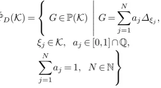
For the reminder of this section, we demonstrate numerical experiments using simulated data (See [9]
for more details). We will take the vector of true
parameters to be θ= (ϵs,ϵ1,τ)T and we will denote
the nodes of the Dirac masses as ξm=k0m. We will
use the simulated data to discuss the importance of the placement of nodes of the Dirac measures, i.e.,
the values of k0j,j= 1,2,···,N. the true probability
measureG0=
∑3
m=1αmk0mwith
α1=α2= 0.05,α3= 0.9,
k01= 570,k02= 580,k03= 850.
We used the true parametersθ0= (2.7,1.9,0.03)T, and
νj was chosen as a realization of a normally
dis-tributed random variable with mean 0 and standard
deviation σ0= 0.005. In all of the experiments, the
data was generated by evaluating equation (10). The
number of division of wavenumbers kj was taken as
n= 70 provided with
kj= 400 + 10×j forj= 0,1,···,n. (20)
From the physical point of views, we impose the
ad-ditional constraint that ϵs> ϵ∞. The parameters
and the distribution were estimated over the range
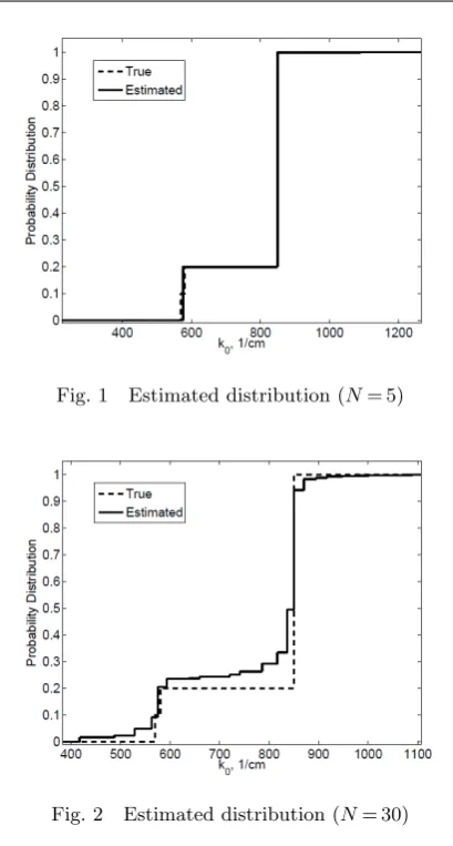
N∈[5,30], and the results are summarized in Table 1
and Figs. 1 and 2.
Table 1 Test results of estimated parameters using PMF
N ϵs ϵ∞ τ
5 2.67 1.88 0.0298
10 2.67 1.87 0.0297
20 2.66 1.83 0.0303
30 2.67 1.84 0.0389
Fig. 1 Estimated distribution (N= 5)
Fig. 2 Estimated distribution (N= 30)
4.
Inverse Analysis using MCMC
Inverse analysis using MCMC methods have been studied and is somewhat different from the PMF ap-proach discussed in the previous section. Let us as-sume the deterministic model (2) and the observation
model (6) with the unknown standard deviationσeof
the measurement errors. In the sequel, the unknown
parameter vector θincludes the resonance
wavenum-berk0and the residual errorσe. For the convenience
of discussions, we use the same notation but five di-mensional parameter vector, i.e.,
θ={θi}
5
i=1={k0,ϵ∞,ϵs,τk,σe} (21)
which is assumed to be a random vector on the
prob-ability triple (Ω,F,P). In this approach, the full
probability model for the unknown parameter vector (21) is adopted instead of the stochastic permittivity model given by (9). Assuming that random variables
θi are mutually independent, the joint distribution of
the vectorθcan be described by
dG(θ)
dθ =
5
∏
i=1
dGi(θ)
dθi
=
5
∏
i=1
gi(θi) (22)
where gi(θi)(i= 1,2,···,5). denote the associated
pri-ori density functions. Noting that measurement
er-rors Vj are independent and normally distributed
with zero mean and unknown constantθ5=σe, the
as-sociated likelihood ratio function can be represented by
l(y0,y1,···,yn|θ)∝ n
∏
i=0
exp [
− 1
2θ2
5
{yj(kj;θ)−yj} 2
]
. (23)
where yj is a realization of Yj. From the Bayes
for-mula, the posterior probability density functionphas
the representation
p(θ|y0,y1,···,yn)∝l(y0,y1,···,yn|θ) 5
∏
i=1
gi(θi). (24)
Consequently, our inverse problem is stated as follows:
(IP): Given a priori distribution g(θ) =∏5i=1gi(θi)
and the collection of the measurement data{yj}nj=0,
estimate the posterior densityp(θ|y0,y1,···,yn) of
un-known quantities in dielectric parameters.
An estimation algorithm can be performed by sampling procedures for the posteriori distribution given by Eq.(24) from which sample paths can be drawn using Markov Chains. There are many alterna-tive algorithms of MCMC, such as Metropolis-Hasting (MH), and Gibbs sampling methods [11]. Our prior efforts on material characterizations exist using in-dependent Metropolis-Hastings [13], gPC Galerkin method [17], and the stochastic spline Galerkin
method [18]. A scheme using Hamiltonian Monte
Carlo method (HMC) is well suitable by making use of gradient information to reduce random walk behavior [19].
The reminder part of this section is to show some experimental results from our previous efforts in [14].Experimental data were generated using the de-terministic model (2) and the observation model (6)
with “true” parameter vector θ0 listed in Table 2.
The number of division of wavenumberskj was taken
as the same one in (20). The nonlinear hierarchical models used in the inversion technique were set as:
yj∼Normal(h(ki;θ), σe),
θi∼Uniform
( θLi, θUi
)
, fori= 1,···,4
θ5∼InvGamma(α,β),
1 2 3 4 5
0.0
0.2
0.4
0.6
0.8
1.0
density.default(x = eps_s)
N = 7500 Bandwidth = 0.06068
Density
Fig. 3 Marginal density of dielectric constant at zero fre-quencyϵs
1.0 1.5 2.0 2.5 3.0
0.0
0.2
0.4
0.6
0.8
1.0
1.2
1.4
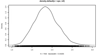
density.default(x = eps_inf)
N = 7500 Bandwidth = 0.04305
Density
Fig. 4 Marginal density of dielectric constant at infinite frequencyϵ∞
Table 2 Test results of estimated parameters (mean val-ues)
Parameter True Estimate
k0 560 557
ϵ∞ 1.90 1.85
ϵs 2.70 2.64
τk 0.03 0.03
σe 0.10 0.10
5.
Concluding Remarks
Stochastic inverse methodologies for dielectric components of composite materials were summarized. The physical model given by the Lorentz oscilla-tor model with unknown parameters was constructed in order to implement stochastic inverse problems. Comparison of two alternative methods for identify-ing unknown parameters in the Lorenz model were
considered. First the existence of uncertainties in
the Lorentz model was formulated by stochastic rel-ative permittivity for the Lorentz model. Then the the treatment of the identification problem consid-ered here was to identify a probability measure on the resonance wavenumber as well as the physical
parameters within the model. The Prohorov
Met-ric Framework played an essential role in the first method. The advantage of this method is that it pos-sesses theoretical convergence of the computational
method summarized here. The experimental results yielded those that were very close to the correspond-ing true distributions. The related feasibility studies were also performed using inorganic glass data in [9]. The second method based on the MCMC sam-pling method was also applied to the same Lorentz model. In the second method, unknown quantities in the physical parameters were assumed to be given by the full probability density model while the rela-tive permittivity was given by a deterministic model. Feasibility studies were carried out illustrating the method with computational experiments using the same simulated data. The second method has the advantage of the consistency of estimated values. In fact, the estimated marginal densities from extracting sampling results were able to provide the reliability and uncertainty quantification for the associated in-verse solutions. The method treated here is directly applicable to the practical identification problems like human muscle tissue which are under study. Inverse analysis including both uncertainties on models and parameters will hopefully become more realistic and practical.
Acknowledgements
This research was supported in part for the first author by the U.S. Air Force Office of Scientific Re-search under grant AFOSR FA9550-18-1-0457. Part of this research was carried out while the second au-thor was visiting at Center for Research in Scientific Computation (CRSC), North Carolina State Univer-sity. Additional support for the second author was also provided by the JSPS Core-to-Core Program, A. Advanced Research Networks, “International re-search core on smart layered materials and structures for energy savings”.
References
[1] H. T. Banks, M. W. Buksas and T. Lin, Electromag-netic Material Interrogation using Conductive In-terface and Acoustic Wavefronts, SIAM Publishers, (2000)
[2] P. Baldus, M. Jansen, and D. Sporn: Ceramic fibers for matrix composites in high-temperature engine ap-plications;,Nature, Vol. 285, pp. 699–703 (1999) [3] H. Ohnabe, S. Masaki, M. Onozuka, K. Miyahara,
and T. Sasa: Potential application of ceramic matrix composites to aero-engine components; Composites Part A: Applied Sciences and Manufacturing, Vol. 30 pp. 489–496 (1999)
[4] H. T. Banks and K. L. Bihari: Modeling and esti-mating uncertainty in parameter estimation;Inverse Problems, Vol. 17, pp. 95–111 (2001)
[5] H. T. Banks and N. L. Gibson: Electromagnetic in-verse problems involving distributions of dielectric mechanisms and parameters; Quarterly of Applied Mathematics, Vol. 64, pp.749–795 (2006)
En-gineering, Chapman and Hall/CRC Press, Boca Ra-ton, (2012)
[7] H. T. Banks, S. Hu, and W. C. Thompson: Modeling and Inverse Problems in the Presence of Uncertainty, Chapman & Hall, (2014)
[8] H. T. Banks, J. Catenacci, and A. Criner: Quan-tifying the degradation in thermally treated ceramic matrix composite; International Journal of Applied Electromagnetics and Mechanics, Vol. 52, No. 1, pp.3–24 (2016)
[9] H. T. Banks, J. Catenacci, and S. Hu: Estima-tion of distributed parameters in permittivity mod-els of composite dielectric materials using reflectance;
Journal of Inverse and Ill-posed Problems, Vol. 23, No. 5, pp.491–510 (2017)
[10] W. R. Gilkes, S. Richardson, and D. J. Spiegelhal-ter (eds.): Markov Chain Monte Carlo in Practice, Chapman & Hall, 1996
[11] D. Gamerman:Markov Chain Monte Carlo, Stochas-tic Simulation for Bayesian Inference, Chapman & Hall, New York, 1997
[12] F. Kojima and S. Kamezaki: Identification of de-fect profiles using a inspection model and informative distributions;Proc. 35th ISCIE International Sympo-sium on Stochastic Systems Theory and Its Applica-tions, ISCIE, pp. 235–240, (2004)
[13] F. Kojima and J. S. Knopp: Inverse problem for electromagnetic propagation in a dielectric medium using Markov Chain Monte Carlo Method; Interna-tional Journal of Innovative Computing, Information and Control (IJICIC), Vol. 8, No. 3B, pp. 2339–2346, (2012)
[14] F. Kojima and H. T. Banks: Statistical parameter estimation of dielectric materials using MCMC for nonlinear hierarchical models; International Journal of Applied Electromagnetics and Mechanics, Vol. 52, No. 1, pp. 49–54, (2016)
[15] H. T. Banks and G. A. Pinter: A probabilistic mul-tiscale approach to hysteresis in shear wave propaga-tion in biotissue; SIAM J. Multiscale Modeling and Simulation, Vol. 3, pp. 395–412, (2005)
[16] Y. V. Prohorov: Convergence of random processes and limit theorems in probability theory; Theor. Prob. Appl., Vol. 1, pp. 157–214 (1956)
[17] F. Kojima, Y. Fujiwara, and T. Usami, Inverse analysis for dielectric medium of conducting mate-rials using generalized polynomial Chaos Galerkin method,Proc. SICE Annual Conference 2014, Sap-poro, Japan, 2014.
[18] F. Kojima and T. Usami, Estimation of dielectric parameters in composite materials using stochastic Galerkin method, Proc. SICE Annual Conference 2015, Hangzhou, China, 2015.
[19] R. M. Neal: MCMC using Hamiltonian Dynamics,
Handbook of Markov Chain Monte Carlo, Eds. S. Brooks, A. Gelman, G. Jones, and X. Meng, Chap-man & Hall, CRC Press, London, 2011
[20] Stan Development Team, Stan Modeling Language Users Guide and Reference Manual, Ver. 2.6.0,
http://mc-stan.org/ February 2015.
Authors
Hardy Thomas Banks (Non-member)
Dr. H.T. Banks is Associate Director of the Center for Research in Scientific Computation at North Carolina State University where he is also a Distin-guished University Professor and LeRoy B. Martin, Jr. Distinguished Professor. Prior to serving as the Director of the Center for Research in Scientific Computation (CRSC) from 1992 until 2018, he spent three years on the faculty at the University of Southern California where he was founder and the first Director of the Center for Applied Mathematical Sciences (CAMS) after having spent over 20 years on the faculty at Brown University. Dr. Banks has published over 500 pa-pers in applied mathematics and engineering journals and written six books. He has served on a number of editorial boards including Computational and Applied Mathemat-ics, Quarterly of Applied Math, Inverse Problems, Journal of Inverse and Ill-posed Problems, Applied Mathematics Letters, International Journal of Mathematical and Com-putational Modeling, Mathematical Biosciences and Engi-neering and was the Founding Editor-in-Chief of the SIAM Frontiers in Applied Mathematics. Dr. Banks is a Fellow of the IEEE, Institute of Physics, SIAM and AAAS. He was the recipient of the IEEE Control Systems Technology Award in 1996, Purdue University Distinguished Alumni Award in 1998, and the W.T. and Idalia Reid Prize in Mathematics from SIAM in 2002. Dr. Banks’ research interests include Inverse Problems and Control for PDE, Modeling in Electromagnetics, Structures, Fluids, and Bi-ology.
Fumio Kojima (Honorary member)