3D Object Reconstruction using Multi-View Calibrated Images

(1)

University of Windsor University of Windsor

Scholarship at UWindsor

Electronic Theses and Dissertations Theses, Dissertations, and Major Papers

2010

3D Object Reconstruction using Multi-View Calibrated Images

Mohammad R. Raeesi N. University of Windsor

Follow this and additional works at: https://scholar.uwindsor.ca/etd

Recommended Citation Recommended Citation

Raeesi N., Mohammad R., "3D Object Reconstruction using Multi-View Calibrated Images" (2010). Electronic Theses and Dissertations. 8044.

https://scholar.uwindsor.ca/etd/8044

(2)

3D Object Reconstruction using

Multi-View Calibrated Images

b y

M o h a m m a d R. Raeesi N.

A Thesis

Submitted to the Faculty of Graduate Studies

through Electrical and Computer Engineering

in Partial Fulfillment of the Requirements for

the Degree of Master of Applied Science at the

University of Windsor

Windsor, Ontario, Canada

2010

(3)

**1 * 1**

Library and Archives Canada Published Heritage Branch Bibliothgque et Archives Canada Direction du

Patrimoine de I'gdition

395 Wellington Street Ottawa ON K1A 0N4 Canada

395, rue Wellington Ottawa ON K1A 0N4 Canada

Your file Votre reference

ISBN: 978-0-494-62747-1

Our file Notre reference

ISBN: 978-0-494-62747-1

NOTICE: AVIS:

The author has granted a

non-exclusive license allowing Library and Archives Canada to reproduce, publish, archive, preserve, conserve, communicate to the public by

telecommunication or on the Internet, loan, distribute and sell theses

worldwide, for commercial or non-commercial purposes, in microform, paper, electronic and/or any other formats.

L'auteur a accorde une licence non exclusive permettant a la Bibliotheque et Archives Canada de reproduce, publier, archiver, sauvegarder, conserver, transmettre au public par telecommunication ou par Nnternet, preter, distribuer et vendre des theses partout dans le monde, a des fins commerciales ou autres, sur support microforme, papier, electronique et/ou autres formats.

The author retains copyright ownership and moral rights in this thesis. Neither the thesis nor substantial extracts from it may be printed or otherwise reproduced without the author's permission.

L'auteur conserve la propriete du droit d'auteur et des droits moraux qui protege cette these. Ni la these ni des extraits substantiels de celle-ci ne doivent etre imprimes ou autrement

reproduits sans son autorisation.

In compliance with the Canadian Privacy Act some supporting forms may have been removed from this thesis.

While these forms may be included in the document page count, their removal does not represent any loss of content from the thesis.

Conformement a la loi canadienne sur la protection de la vie privee, quelques formulaires secondaires ont ete enleves de cette these.

Bien que ces formulaires aient inclus dans la pagination, il n'y aura aucun contenu manquant.

M

(4)

Author's Declaration of Previous Publication

This thesis includes one original paper that has been previously submitted for

publication in peer reviewed conference, as follows:

Thesis Chapter Full Citation Publication Status

Chapter 4 Mohammad R. Raeesi N., Q. M. Jonathan Wu, "A Complete Visual Hull Model Using Bounding Edges", Pacific Rim Conference on Multimedia 2010.

Submitted

I certify that I have obtained a written permission from the copyright owner(s) to

include the above published material(s) in my thesis. I certify that the above material

describes work completed during my registration as graduate student at the University of

Windsor.

I declare that, to the best of my knowledge, my thesis does not infringe upon

anyone's copyright nor violate any proprietary rights and that any ideas, techniques,

quotations, or any other material from the work of other people included in my thesis,

published or otherwise, are fully acknowledged in accordance with the standard

referencing practices. Furthermore, to the extent that I have included copyrighted

material that surpasses the bounds of fair dealing within the meaning of the Canada

Copyright Act, I certify that I have obtained a written permission from the copyright

owner(s) to include such material(s) in my thesis.

I declare that this is a true copy of my thesis, including any final revisions, as

approved by my thesis committee and the Graduate Studies office, and that this thesis has

(5)

Abstract

In this study, two models are proposed, one is a visual hull model and another one

is a 3D object reconstruction model. The proposed visual hull model, which is based on

bounding edge representation, obtains high time performance which makes it to be one of

the best methods. The main contribution of the proposed visual hull model is to provide

bounding surfaces over the bounding edges, which results a complete triangular surface

mesh. Moreover, the proposed visual hull model can be computed over the camera

networks distributedly. The second model is a depth map based 3D object reconstruction

model which results a watertight triangular surface mesh. The proposed model produces

the result with acceptable accuracy as well as high completeness, only using stereo

matching and triangulation. The contribution of this model is to playing with the 3D

(6)

Dedication

This thesis is dedicated to my beloved parents, who have raised me to be the

person I am today. You have been with me every step of the way, through good times

and bad. Thank you for all the unconditional love, guidance, and support that you have

always given me, helping me to succeed and instilling in me the confidence that I am

(7)

Acknowledgements

I would like to thank all people who have helped and inspired me during my

graduate study.

I especially want to thank Dr. Jonathan Wu, my supervisor, for his support and

guidance throughout this entire thesis process and for believing in my abilities. Dr.

Shervin Erfani and Dr. Nader Zamani deserve special thanks as my thesis committee

members. Thank you for your support and guidance.

I am indebted to all of my roommates during past two years for their friendship,

care and support. I would like to thank Abbas Ghaei, Amir Hassannejadasl, Ali

Aryanpour, and especially Esmaeal Navaei. Good luck to each of you in your future

endeavors.

My deepest gratitude goes to my family for their unflagging love and support

throughout my life; this dissertation is simply impossible without them. I am indebted to

my parents, for their care and love. I cannot ask for more from them, as they are simply

perfect. I have no suitable word that can fully describe their everlasting love to me. I

remember their constant support when I encountered difficulties. I feel proud of my

family, for their support and care in my whole life.

Last but not least, thanks to God for my life through all tests in the past two years.

You have made my life more bountiful. May your name be exalted, honored, and

(8)

List of Figures

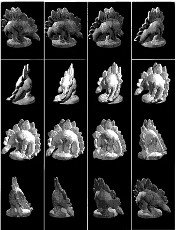
Figure 1-1. Sample views of DinoSparseRing dataset [2] 2

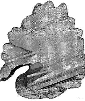
Figure 1-2. 3D convex hull for DinoSparseRing dataset 2

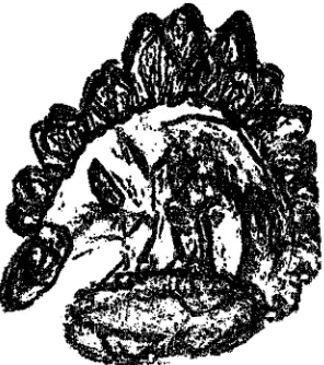
Figure 1-3. Visual hull model of DinoSparseRing dataset 3

Figure 1-4. Surface points for DinoSparseRing dataset 4

Figure 2-1. Sample view (a) of Dinosaur dataset and its silhouette image (b) [7] 7

Figure 2-2. The polyhedron representation of a plastic horse produced by Baumgart [6]. 7

Figure 2-3. Sample application of chromakeying 8

Figure 2-4. Intersection of silhouette cones 9

Figure 2-5. Two different images with the same silhouette set 10

Figure 2-6. The division of Laurentini of the object surfaces [12] 11

Figure 2-7. Reconstructed visual hull based on different number of views [13] 11

Figure 2-8. A simple octree structure to model the 3D object [16] 13

Figure 2-9. The synthetic objects and their octree models produced by R. Szeliski [16]. 13

Figure 2-10. Two rims intersecting at a frontier point [19] 15

Figure 2-11. The silhouette image and the corresponding edge-bin structure [20] 16

Figure 2-12. The results of the proposed algorithm in [13] on a torus in different number

of views with the processing time 16

Figure 2-13. A sample slice of the image based visual hull [21] 17

Figure 2-14. The rays and their corresponding projected rays [22] 18

Figure 2-15. A bounding edge through the first camera [23] 18

Figure 2-16. A sample view of a 3D object and corresponding bounding edge model from

two views [11] 19

Figure 2-17. A sample view of a 3D object and the corresponding colored surface points

from two different views [11] 21

Figure 2-18. Forward and backward moving of the colored surface points have been

(12)

Figure 2-19. Combining silhouette images from different time instances, by moving the

center of the cameras backward [11] 23

Figure 2-20. Sample image pairs for stereo vision [24] 27

Figure 2-21. The ideal depth map for sample pairs [24] 27

Figure 3-1. A sample view ofMeshLab application 29

Figure 3-2. Images of Dinosaur dataset 31

Figure 3-3. Images of Predator dataset 32

Figure 3-4. DinoSparseRing dataset images 33

Figure 3-5. Resulted silhouette images for Dinosaur dataset 35

Figure 3-6. Resulted silhouette images for Predator dataset 36

Figure 3-7. Resulted silhouette images for DinoSparseRing dataset; sample images (1st

row), results of providers suggestion (2nd row), manually refined results (3rd row) 37

Figure 4-1. (a) The bounding edge model for the 1st view of Dinosaur dataset and (b)

corresponding contour map 42

Figure 4-2. The silhouette of the 1st view of Dinosaur dataset (left) and the inconsistent

pixels which are the difference between the input silhouette and the consistent one (right).

44

Figure 4-3. Intersection of the occupancy intervals form different viewpoints 46

Figure 4-4. Bounding surfaces resulted for the first 8 views of Dinosaur dataset 48

Figure 4-5. Bounding surfaces resulted for the first 8 views of Predator dataset 48

Figure 4-6. Bounding surfaces resulted for the first 8 views of DinSparseRing dataset.. 49

Figure 4-7. Final triangular meshes for Dinosaur datasets 49

Figure 4-8. Final triangular meshes for Predator datasets 50

Figure 4-9. Final triangular meshes for DinoSparseRing dataset 50

Figure 5-1. Ground truth for DinoSparseRing dataset [2] 56

Figure 5-2. Dinosaur sample image pair 63

Figure 5-3. Rectified Dinosaur image pair 63

Figure 5-4. Rectified silhouette image pairs 64

Figure 5-5. Left-to-right (left image) and right-to-left (right image) depth maps produced

(13)

Figure 5-6. Left-to-right depth map (left image) and resulted depth map after LRC check

(right image) for the sample image pairs of Dinosaur dataset 66

Figure 5-7. Reconstructed 3D points for the first view of Dinosaur dataset 66

Figure 5-8. Refined 3D points for the first view of Dinosaur dataset 68

Figure 5-9. Resulted 3D surface points for Dinosaur dataset 70

Figure 5-10. Resulted 3D surface points for DinoSparseRing dataset 70

Figure 5-11. The inconsistent image of DinoSparseRing dataset 71

Figure 5-12. Final 3D triangular mesh for DinoSparseRing dataset 71

Figure 5-13. Final 3D triangular mesh for DinoSparseRing dataset from different views.

72

Figure B - l . Accuracy comparison among all the state-of-the-art methods 94

Figure B-2. Completeness comparison among all the state-of-the-art methods 95

Figure B-3. Accuracy comparison among the depth map based methods 95

Figure B-4. Completeness comparison among the depth map based methods 96

Figure B-5. Accuracy comparison among the methods which are not published yet 96

Figure B-6. Completeness comparison among the methods which are not published yet.

(14)

List of Tables

Table 2-1. The comparison of different visual hull models 24

Table 4-1. Numbers of inconsistent points for the first 8 views of the Dinosaur dataset. 43

Table 4-2. Number of vertices in the all surfaces versus the merged surfaces before

re-meshing 51

Table 4-3. Execution time of the final visual hull model produced by different models in

second 51

Table 4-4. Execution time sequentially versus distributedly in second 53

Table 5-1. Evaluation results of both proposed models on Middlebury benchmark for

DinoSparseRing dataset. The accuracy is in millimeter and completeness is percentage. 73

Table 5-2. Comparison of accuracy of the state-of-the-art models. The accuracy threshold

is 90% 74

Table 5-3. Comparison of completeness of the state-of-the-art models. The completeness

threshold is 1.25mm 75

Table 5-4. Comparison of accuracy of the state-of-the-art depth map based models. The

accuracy threshold is 80% 76

Table 5-5. Comparison of completeness of the state-of-the-art depth map based models.

The completeness threshold is 1.5mm 77

Table A - l . Class files implemented in Java with number of physical and logical lines of

(15)

1. Introduction

There are many applications such as obstacle avoidance in robotics, 3D modeling

in inverse engineering, assisted living, security and surveillance which need to localize,

recognize, reconstruct and track the 3D objects. There are many approaches for these

applications, such as marker-based tracking which attaches some markers to the

interesting objects. Some of the existing approaches are not applicable in many

environments; for example, it is not possible to use the marker-based approaches for

surveillance applications in public places. The best, applicable approach is vision

network, because it is relatively cheaper, and it can be configured easily [1].

The area of these applications is quite wide, including Electrical Engineering,

Computer Science, Mechanical Engineering, Medicine, and Security. The goal of all of

these applications is to reconstruct the 3D object, but each of them needs the geometric

information of the 3D object in different level of details. In obstacle avoidance

applications in robotics, for example, moving robot gets the information from the

environment using its sensors, and based on the received information it chooses a path to

reach the destination without hitting the existing obstacles. Since the robot only needs the

location and the course information of the shape of the 3D objects just to move along the

objects, there is no need to recover the exact shape of the 3D object. Controversially, in

3D modeling for inverse engineering, the shape of the object and all geometrical

information of it should be reconstructed as accurate as possible. Considering the

processing time, the reconstruction should be real time for moving robots, while there is

no limitation for 3D modeling applications.

In vision networks, there are different algorithms which will result in different 3D

reconstructed shape of the object, from a coarse model to the most precise one. The

applications in this field recover the 3D shape of the objects based on the captured

images from different views of the object. Most of them use the silhouette images to do

(16)

information from each image, computing a model of the objects in the scene, representing

the objects and making decision about the situation of the objects in the scene.

The inputs used for vision network applications are multi-view calibrated images.

Camera calibration is a part of vision network applications which is out of the scope of

this study. Figure 1-1 shows sample images from DinoSparseRing dataset [2].

c

Figure 1-1. Sample views of DinoSparseRing dataset [2].

The coarsest model in camera networks is 3D convex hull. The 3D convex hull of

a set of 3D points is the smallest subset of the space such that for any two points u and v,

the segment joining them is completely in the subset. Consider DinoSparseRing dataset,

for example, the resulted 3D convex hull has been shown in Figure 1-2.

Figure 1-2.3D convex hull for DinoSparseRing dataset.

(17)

A better 3D model for the reconstructed object is visual hull model which is

described in the next section as a fundamental concept in 3D reconstruction field. As an

overall view, visual hull is the best approximation of the object based on the binary

images of the object without any color information. Figure 1-3 shows the resulted visual

model for the DinoSparseRing dataset. As it can be seen clearly, the visual hull model is

more precise than the convex hull. In other words, visual hull is much more similar to the

3D object than the convex hull model.

Figure 1-3. Visual hull model of DinoSparseRing dataset.

The 3D reconstructed object is the name of the best model for representing an

interesting 3D object, which shows all the concavities of the 3D objects. This model

represents all geometric information of the object as accurate as possible. To produce 3D

reconstructed object, all the information captured by the cameras will be used including

color information. A sample view of the best reconstructed surface points of

DinoSparseRing dataset has been shown in Figure 1-4.

The 3D reconstructed object model is the most similar model to the 3D object. As

providing more detailed information needs more processing, the execution time of the 3D

reconstructed object is much higher than the visual hull and convex hull models.

(18)

Figure 1-4. Surface points for DinoSparseRing dataset

In this thesis, I propose two new algorithms, one is a visual hull model and the

other one is a 3D reconstructed object model. The proposed visual hull model produces a

complete triangular mesh based on the bounding edge model, which is the fastest visual

hull model in the existing approaches. The time performance of the proposed model is

better than the most existing approaches which provide the same type of results. For the

second model, I used depth maps to reconstruct the 3D surface points of the object. To

have the reliable depth map, I did a survey in stereo vision to select the best way to do so.

Before describing the proposed models, fundamental concepts are reviewed in

section 2. Implementation platform including programming methodology and datasets are

mentioned in section 3. Section 4 describes the proposed visual hull model and the

obtained results and evaluation. The 3D reconstructed object model is described in

section 5, followed by the conclusions in section 6. The last part, Appendix A, describes

the implemented codes in Java programming language.

I used Matlab and Java programming languages to implement the codes of the

proposed algorithms. Because Matlab is much faster than Java for matrix manipulation, I

used Matlab for image processing tasks, such as window matching. For the 3D

computation, Java is used which is faster than Matlab in this case. The Matlab version

used is 7.0.0.19920(R14), and the Java version is 1.6.0_12.

(19)

2. Fundamental Concepts

W. N. Martin and J. K. Aggarwal [3] first described the volumetric description

from multiple views. Later, other researches defined the fundamental concepts of the 3D

model approximation, such as silhouette and visual hull. These concepts are used in all of

the corresponding algorithms.

To provide the multi-view calibrated images, as the input for 3D object

reconstruction, there are two approaches. The first one is to use a turntable to rotate the

object and a camera to capture images. The second approach is to configure a camera

network on the environment under study. If a processing unit is available for the camera

nodes in the network, the computation of the algorithms can be distributed over the

network. Otherwise, there is a server which processes the captured images from different

cameras.

2.1. Distributed Vision Network

The most significant concept to be defined is the Distributed Vision Network. In

this study, the definition of the Distributed Vision Networks is the same as the definition

of A. Mavrinac [4]. Distributed Vision Networks are networks of dispersed camera

nodes. Each node has (i) a camera module for image acquisition, (ii) a processor to

process the raw image locally, and (iii) a communication module to send and receive

information. This type of network can either use a central device to perform collective

processing of the data or perform the processing collaboratively by the nodes. The

cameras are calibrated over the network. Camera calibration, also called camera

resectioning, is the process of finding the true parameters of the cameras that produced a

given photograph or video. Camera parameters include the focal length, point of view,

global position, global direction, and global rotation. Camera calibration may be done

(20)

The field of distributed vision networks is a new and growing field, which is still

in the beginning stages of research. This field is a combination of several fields including

computer vision, image processing, distributed computing, embedded systems, data

networks and communications. This combination adds new opportunities from the union

of the fields and new limitations imposed by their intersections [4].

It this study, I consider distributed computing as well as centralized one. The

performance of the proposed visual hull model is evaluated on the both types of

networks. For the 3D reconstructed object model, all the computations are done

sequentially on a centralized server. In this case, a set of camera stations send their

captured images to the server and server reconstructs the 3D shape of the objects based

on the received images and camera parameters.

2.2. Distributed Computing

Using the distributed computing network environment is beneficial for the Vision

Networks in some ways. Distributed computing makes the networks to be scalable. It

avoids transmitting the raw images, which have so huge amount of data. In addition, it

can preserve the privacy of the network users in some applications such as assisted living.

Also, it enhances the flexibility on the type of feature and level of exchanging data. So

we will have the fusion across the three dimensions; 3D space (different camera views),

time (collecting the data over time) and feature levels (selecting and fusing different

feature subsets) [5]. As mentioned before, I consider distributed computing only for the

evaluation of the proposed visual hull model. In this case, the first step of the algorithm is

computed over the camera nodes in parallel, while the next step which is the merging step

is done on a centralized server.

2.3. Silhouettes

All of the existing algorithms use the silhouette concept to get the information

(21)

foreground or background. The scene background pixels are most often colored as white,

while the foreground pixels are colored as black. These foreground pixels are related to

the interesting objects in the scene. Baumgart [6] first considered silhouettes to

approximate a polyhedron representation of the objects. He called his work as inverse

computer vision, because computer vision generates synthetic images from the real

world, while 3D object reconstruction uses the captured images to reconstruct the real

object with all the geometric information. A sample silhouette image with its

corresponding image has been shown in Figure 2-1.

Baumgart [6] used three captured images from a plastic horse on a turntable to

draw the silhouette images. Then by using the silhouette cone intersection, he produced a

polyhedron model of the object. He mentioned that silhouette cone intersection looks like

carving a statue by cutting away everything not related to the object. Figure 2-2 shows

the 3D reconstructed object using Baumgart techniques. His result polyhedron looks like

a statue of a horse which is not completed yet. It seems to be cut by knife.

(a) (b)

Figure 2-1. Sample view (a) of Dinosaur dataset and its silhouette image (b) [7].

(22)

There are two common ways to produce the silhouette from the captured images

which include chromakeying and background subtraction. However, in some recent

work, the silhouettes are computed manually using Adobe Photoshop, just to

segmentation of the foreground and background pixels.

The first approach, chromakeying, also called bluescreen matting. In this

approach the background is a single uniform color which does not appear in the

foreground objects. So by checking the color and compare it with the background color, it

is possible to compute the silhouette of the object. This method can not be used in many

applications, because of its limitation on the background color, but it is applicable in

cinematic special effect and television weather forecasts [8]. A sample application of

bluescreen matting has been shown in Figure 2-3. The selected color for the background

is green, while there is no green pixel for the foreground object. So only by a comparison

of the color of the pixels, it is possible to detect the background pixels and change their

value to provide a special effect.

Figure 2-3. Sample application of chromakeying.

Another common way is background subtraction. In this method, first the

statistical model of the background is produced by capture many images from the

background. So it is possible to detect the foreground objects by comparing the new

(23)

new image is greater than the corresponding threshold, that pixel will be considered as a

foreground pixel [9].

For some datasets, the dataset providers provide the contour information of the

silhouettes as well as the image data. The contour information is a set of pixels which are

not connected. The connected version of these pixels represents the silhouette contour. I

implement a function to produce the best connected version of these pixels. Then based

on the resulted silhouette contours, the silhouette image is produced. Other datasets

suggest the best way to produce the silhouette information. These methods will be

described later.

Silhouette images are very efficient for vision networks in case of

communication, because their size is much smaller than the size of the raw images. For

example, a 2000x1500 color image is approximately 400KB, while a silhouette image

with the same resolution (without any compression) is less than 8KB.

2.4. Visual Hull

The constructed objects of the silhouettes is called visual hull. Visual hull concept

was first defined by A. Laurentini [10]. Visual hull is the intersection of the silhouette

cones, which are the cones started from the camera positions and goes through the

silhouette contours. Figure 2-4 shows the silhouette cones from different viewpoints with

different colors. The intersection of all the silhouette cones is called visual hull model of

the object.

A

(24)

Based on the silhouettes information, visual hull is the best approximation of the

interesting object. Because visual hull is constructed from the silhouette images, it is also

called Shape from Silhouette (SFS). Visual hull is the maximal one of the objects which

has the same set of silhouettes as the given one. In other word, it is possible for many

objects to have the same set of silhouettes; visual hull represents the maximal object. So,

it is not possible to identify the objects only based on the silhouette, especially for the

non-convex objects. Figure 2-5 shows two different objects which have the same set of

silhouettes. So based on the silhouette information, there is no way to recognize any of

them.

The visual hull applications and the resulted models are very sensitive to

silhouette noise and camera calibration errors.

G. Cheung et al. [11] defined a consistency concept for the set of silhouette

images. The set of silhouette images is consistent, if there is at least one non-empty

volume that exactly explains all the silhouette images. Because there are many objects

that have the same set of silhouettes, G. Cheung defined the visual hull as the largest

possible volume which exactly explains the silhouette images.

A. Laurentini [12] divided the surfaces of a volume into two categories,

silhouette-active surface and silhouette-inactive surface. The former is what can be

reconstructed by the silhouette cone intersection, while the latter one is what can have

any shape without affecting the silhouettes of the object. The following figure shows an

example of this division. Figure 2-6(a) and (b) shows the two categories of surfaces. The

(25)

images. So the resulted visual hull in the best situation is what has been shown in Figure

2-6(c), while the real object is one has been shown in Figure 2-6(d).

• -p. • I silhouette-active surface

• silhouette-inactive surface

(») 0 ) («) (<)

Figure 2-6. The division of Laurentini of the object surfaces [12].

The accuracy of the visual hull mainly depends on the number of silhouette

images and their corresponding camera positions. The visual hull will be tighter if the

number of silhouette images is increased. The greater the number of the views, the more

precise the approximated visual hull. Figure 2-7 shows different reconstructed visual

hulls based on different number of views. It also shows the execution time of

reconstruction for each set. The execution time is increased by increasing number of

views more rapidly.

i ti:

4 views 119 ma

1 \

' • ' ' J/

12 vfcnra I tit at* 16 views / 217 na 42 view« / 1.44 s I view* J7ins

Figure 2-7. Reconstructed visual hull based on different number of views [13].

Based on the survey I did in this field, there are four main categories of visual hull

models. In existing approaches for modeling the visual hull, two categories are popular,

voxel based approaches and surface based (polyhedron) ones. Other categories are

image-based visual hull and bounding edge visual hull. Main existing models are described in

(26)

2.4.1. Voxel Based Visual Hulls

The first category is modeling the objects by a collection of elementary 3D cells.

These cells are called voxels (volumetric pixels), which are first introduced by W. N.

Martin and J. K. Aggarwal [3]. Voxels are classified into two categories, the inside and

the outside one. If voxels are positioned completely outside the visual hull, in other word,

if they have not any intersection at least with one silhouette, they will be classified as

outside voxels. Otherwise, if they intersected partially or completely with all the

silhouette images, they will be classified as inside voxels. Because voxel based model

uses the discrete volumetric representation, it generates some quantization and aliasing

artifacts on the resulting model.

The voxel based approaches improved by introducing octrees. Octrees have been

first introduced by C. L. Jackins and S. L. Tanimoto as an efficient geometric

representation [14]. Then octrees have been used for modeling the objects from three

orthographic projections by C. H. Chien and J. K. Aggarwal [15].

Octrees are tree-structured representations which are used to model the volumetric

data. The octree is constructed by recursively dividing each cube to eight sub-cubes to

cover the interesting volume as accurate as possible. There are three possible locations

for the cubes including inside the volume, outside the volume and on the boundary. If a

cube is completely inside the volume, it will be labeled as inside and its color will be

black. If it is completely outside the volume, it will be labeled as outside and it will be

colored as white. Otherwise, it will be labeled as boundary and be colored as gray. Based

on the application, the gray cubes will be recursively divided to reach the desired

accuracy for modeling the object. Figure 2-8 shows the structure of a sample octree

model [16].

Figure 2-8 represents an octree model by 6 cubes of two consecutive levels. Each

(27)

C MM, 2 4 ^Jtk

10 «0 6i

Figure 2-8. A simple octree structure to model the 3D object [16].

R. Szeliski used the octree representation to model the objects. To have an

efficient algorithm, he first produced a coarse model of the objects and then by dividing

the gray cubes, he refined the model. By using this approach, the number of the trimmed

cubes was decreased. To check the location of the cube, it is necessary to project the cube

to each image plane to check whether it is inside the silhouette or not. The simplest way

is to project the corners of the cube to the image plane and then check the situation of the

projected hexagon against the silhouette. This method is accurate, but it is very time

consuming. R. Szeliski proposed to convert the cube to a bounding square instead of

project its corners. The resulted reconstructed visual hulls of his model have been shown

in Figure 2-9 [16].

Figure 2-9. The synthetic objects and their octree models produced by R. Szeliski [16].

The octree model performs voxel model. With the same storage space, the

(28)

time needed to construct a voxel model is greater than what the octree model needs,

because it evaluates more geometric cells. For representing the reconstructed 3D shape of

the object, octree model is also faster, since the number of its geometric cells is less than

voxel model.

K. Kutulakos and S. Seitz [17] proposed a voxel based algorithm to model the

visual hull. They called it space carving. Space carving algorithm starts on the initial

volume and recursively checks the surface voxels to decide whether to carve them or not.

It continues checking until no voxels is carved in an iteration.

If the silhouette images are noise free, the smaller voxel size results the better

approximation of the visual hull. Otherwise, if the silhouette images are noisy, smaller

voxel size causes more errors in classification. So, the best size of the voxels is highly

dependent to the error of silhouette images [18].

2.4.2. Polyhedral Visual Hulls

The second category of the popular visual hull modeling is surface based one. In

this category, a polyhedron model of the object is produced by intersecting the silhouette

cones. The surfaces of the polyhedron are the visual cone patches, the edges of it are the

intersection curve between two silhouette cone, and the vertices are the points where

more than two silhouette cones intersect. To generalize the polyhedron, it is assumed that

the contour of the object has been oriented counterclockwise, so the object is always at

the left of the contour.

S. Lazebnik et al. [19] proposed two representations for the visual hull of a 3D

object, the rim mesh and the visual hull one. Rim is the surface points of the object where

a ray through the viewing point intersects the object. The projection of the rim to the

corresponding image plane is the silhouette contour. The intersection of two rims could

be isolated points which are called frontier points. The rim concept has been shown in the

following image. They defined the rim mesh by its vertices (the frontier points), edges

(29)

the edges). Figure 2-10 shows two rims from two different points of view which intersect

at a frontier point.

Besides, S. Lazebnik et al. [19] described the difference between the rim mesh

and the visual hull one. Because the rim mesh depends only on the ordering of the

frontier points, it is topologically more stable. While the visual hull meshes recover the

geometry information in a more reliable manner.

* » / ;?

_ . ; frontierpoiat

intersection curve

J. '' i ;

S • ' ' V

/

/ ; 4. > X

„" apparent contours '* r>. J

Figure 2-10. Two rims intersecting at a frontier point [19].

C. Buehler et al. [20] proposed the real time representation of the polyhedral

visual hulls. Their representation is view independent, so it does not need to be

reproduced for a set of silhouette images. It is suited to be computed by the graphics

hardware. They assumed each silhouette is a 2D polygon. For each edge of the polygon,

they compute the face of the silhouette cone. By using the intersection of the face and

other silhouette images, the face of the polyhedron is determined which itself is a

polygon. To intersect the face of the silhouette cone by the other silhouette images, the

edges of the face of the silhouette cone have been projected to the silhouette images. To

accelerate this process, preprocess has been done for each silhouette images. In the

preprocessing step, each silhouette has been divided to the bins. Based on these bins, a

table of the edges-bins is computed. Figure 2-11 shows the divided silhouette image and

the corresponding edge-bins table. The algorithm uses this table to respond as quickly as

possible to the intersection problem. This edge-bin structure can be used for the visibility

(30)

Figure 2-11 shows an example of an edge-bin structure. The silhouette image is

divided into seven bins. The cells of the edge-bin table contain the intersecting edges

which are sorted ascendingly, based on the distance to the epipole increasingly.

bill i //Mtt5X^ hmi / t x X

Em I 2 S 4 5 6 1

Edges 0 1*4 €2- 9

Figure 2-11. The silhouette image and the corresponding edge-bin structure [20].

J. S. Franco and E. Boyer [13] proposed a fast algorithm to represent the best

polyhedral visual hull. They first computed a coarse approximation of the visual hull by

retrieving the viewing edges. Then, they generated the surfaces of the mesh. Finally, they

identified the faces of the polyhedron. They applied their algorithm on a torus for

different number of views. The greater the number of the views, the more precise the

approximated visual hull. Their results have been shown in Figure 2-12. The time needed

to compute each result has been shown as well, which is increased faster than the number

of views.

4 views /19 m* 8 views 175 mi 12 views 1125 us 16 views /217 ms 41 views / 1.44s

(31)

2.4.3. Image-Based Visual Hulls

On of the compact representations of the visual hull is image-based visual hull. C.

Buehler et al. [21] defined the image-based representation as a two dimensional, sampled

representation. For example, a color image is a 2D color samples, or a disparity map in

stereo vision is a 2D disparity samples.

The image-based visual hull is a two dimensional, occupancy intervals samples.

The visual hull is represented by the rays from view points through the image plane.

Instead of storing either foreground or background, the samples are the intervals of the

rays which are inside the visual hull. In other word, the intervals of the ray which

intersect all the other silhouette images are stored in the samples. So for each pixel, the

list of its corresponding intervals is stored. If a pixel is a background pixel, its list will be

empty. Figure 2-13 shows a slice of the image-based visual hull [21].

Figure 2-13. A sample slice of the image based visual hull [21].

The image-based representation has many advantages in comparison to other

models. Its storage requirements and computational complexity are very low, which is

much less than the aforementioned algorithms. It has a simple and fast computation. The

rendering is too simple as well. Because it has two discrete dimensions and one

continuous dimension, it has a higher resolution than the resolution of the voxel based

representation.

W. Matusik et al. [22] proposed an image-based approach to represent the visual

hull. Based on the Calculatus Eliminatus principle, they said that the visual hull

approximation is carving away the regions of space where the object is not. Calculatus

(32)

and it must be in the place we haven't looked. Their algorithm contains three steps. It first

projects the rays from a desire viewing point to the silhouette images. Then, in the second

step, by intersecting the projected rays and the silhouettes, it computes the interesting

intervals. Finally, the intervals are returned to the 3D space. The intersected parts of these

intervals from all the silhouettes will be saved for each pixel. A plot of the projected rays

is shown as follows. Figure 2-14 shows the rays from the point of view of an image

through the interesting pixels and their corresponding projected lines on the plane of

another image. All the projected lines intersect at the epipole, the projected point of the

corresponding point of view.

2.4.4. Bounding Edge Visual Hull

The next visual hull representation is bounding edges. This representation has

been first introduced by G. Cheung [18, 23, 11, 1]. He defined the bounding edge

representation as the parts of the rays from the viewing point through the contour of the

corresponding silhouette image which intersect all the other silhouette images.

Target Image

Figure 2-14. The rays and their corresponding projected rays [22].

(33)

Figure 2-15 shows a bounding edge of first camera for a sample pixel which is

located on the 3D ray from the camera position through the pixel, and is intersected with

other three silhouettes. The starting point SV and finishing point F F will be saved for the

pixel as the endpoints of a bounding edge. To have a better performance, instead of

saving the 3D position of each endpoint, its distance to the camera position will be saved

[23].

Bounding edges are very similar to the based representation. Like

image-based model, it calculates the intervals of the rays from the view point through the

silhouette pixels. However, in contrast to image-based representation, it considers only

the silhouette contour pixels instead of all the silhouette pixels. Image based

representation is view dependent, since it produces the interval samples for only one

view, but bounding edge model produces the edges for all viewpoints. An example of

bounding edge representation has been shown in Figure 2-16 [11].

Figure 2-16. A sample view of a 3D object and corresponding bounding edge model from two views

[Hi-Bounding edges lie exactly on the surface of the visual hull. They intersect the

real object at least at one point. The drawback of this representation is that it is

incomplete. A visual hull is complete, if it has all the geometrical information of its

shape. If visual hull has any holes on its surface, it will be considered as incomplete

model. Since the small amount of accurate data is better than the large amount of the

approximated data, in many applications, an exact visual hull is preferred than the

(34)

It is not necessary for the bounding edges to be continuous. They can consist of

many parts. It exactly depends on the shape of the silhouette images. If all the silhouette

images are convex, the bounding edges will be continuous. The important usage of the

bounding edge representation is refinement of the visual hull across time. G. Cheung et

al. [11] proposed an algorithm to increase the number of silhouettes by capturing more

images of the interesting objects over the time.

2.5. Visual Hull across Time

As mentioned before, the visual hull accuracy depends mainly on the number of

silhouette images. To increase the precision of the visual hull, the number of silhouette

images should be increased. There are two ways to increase the silhouettes number. The

first one is to increase the number of cameras to produce more silhouette images which

has the financial cost and the limitation for the camera positions. The second approach is

using the same cameras across time. G. Cheung et al. [11] proposed an algorithm to

increase the number of silhouette by capturing more images of the interesting objects

over the time. If there are K cameras in the environment, and J frames of each camera are

used, the effective number of silhouette images will be JK instead of K. To apply this

approach, first it is necessary to calculate the motion of the interesting object between the

time instances. Then silhouette images in different time instances can be combined based

on the computed motion over the time. The task of estimating the motion of the object is

called visual hull alignment, and the task of combining the silhouette images is called

visual hull refinement.

G. Cheung et al. [23, and 11] considered two fundamental properties of the visual

hull. The first one, called 1st FPVH (First Fundamental Property of Visual Hull), is that

the 3D object which produces the silhouette images lies completely inside the visual hull.

This property can be used for many applications such as obstacle avoidance in robotic

navigation. The second one, called 2nd FPVH, is that each bounding edge touches the real

(35)

construction of the colored surface points (CSP) possible. To construct the colored

surface points, they combined the 2nd FPVH with the stereo vision concept.

Colored surface points have been first introduced by G. Cheung [18]. CSPs are

the 3D points on the bounding edge which touch the object. The information needed to

find the position of the CSPs through the bounding edge comes from the color

consistency check algorithm. It finds the best point on the bounding edge, the color of

which is consistent in all other color images for which the point is visible. The visibility

is another important issue to refine the visual hull across time. Because at least one point

exists on the bounding edge to touch the object, there is no need to define any threshold.

An error measurement algorithm is applied to find the best point. This error is the

variance of the color of the point from different visible point of view. In noise free

environment, the color variance of a 3D point in all the points of view should be zero.

But in real environment, it is necessary to find the best point with least color variance.

Figure 2-17 represents the visual hull by its colored surface points. These CSPs are on the

surface of the visual hull. In contrast to all other representation, CSPs are colored 3D

points.

Figure 2-17. A sample view of a 3D object and the corresponding colored surface points from two different views [11].

To estimate the motion of the object, G. Cheung et al. [11] used the 3D CSPs. The

algorithm starts with an initial motion, followed by the refinement step. To decrease the

complexity of the algorithm, CSPs are moved forward from the first time instance to the

next one based on the initial motion, and then projected to the images in the second time

instance which is followed by the 3D consistency check. This approach is done in inverse

(36)

the silhouettes of first time instance. Figure 2-18 shows the forward and backward

movement of the 3D CSPs through the time instances.

To refining the motion, G. Cheung et al. [11] used two error measurements

including photometric error and geometric one in both directions, forward and backward.

The forward photometric error is the color difference between the CSPs in the first time

instance and the projected moved points in the second time instance. If the moved points

project in the background section of the corresponding silhouette, the photometric error

will be considered as zero. Because the images may be noisy and there are some errors in

camera calibration in practical cases, they considered valid. For these cases, geometric

error is defined, which is the distance of the projected moved CSPs to the silhouettes.

This error is zero, when the points project inside the silhouette [11].

: Till

Colored SmisMie Touching taint*

{"3D limtgti*")

I n l t i n l m o t i o n e s i i m m o ( R . 1)

t, ^ t,

Error between ihu projected color* on .

2D images at t. «»<! M ; KT W,1 - HT T

lienor becwtxti tfc projected cotors on 2t> image* sit vt and p ,

Figure 2-18. Forward and backward moving of the colored surface points have been shown as well as the corresponding errors [11].

After finding the best approximation of the motion, it's time to combine the

silhouette images, called visual hull refinement. To do so, first a reference time instance

should be set. The first time instance is the best candidate for the reference. The

silhouette images from other time instances are effective silhouette images in reference

time instance, whose points of view are moved, based on the corresponding refined

(37)

lime i, 'time t. i i ,. . • C

( R \ - RTt )

R (C"- I )

RT( C I t

< Rr, - R * t )

Figure 2-19. Combining silhouette images from different time instances, by moving the center of the cameras backward [11].

G. Cheung et al. [11] applied the proposed algorithm on the rigid objects as well

as the articulated objects. The articulated objects are the objects that have many parts

which can move in different directions. The best example of an articulated object is

human body. The joint estimation is separated from the motion estimation to decrease the

complexity of the algorithm. The shape and the motion of all the object parts are

computed individually, and then the position of the joints are localized.

2.6. Comparison

The four different representations of visual hull have been described. The entities

of the representations are different. The voxel-based one represents the visual hull by the

cube cells, while the polyhedral representation models it by the faces, edges and vertices

of the polyhedron. The image-based visual hull consists of a two dimensional interval

samples, and the bounding edge model represents the visual hull by the bounding edges

from different viewpoint.

The comparison of the visual hull models has been shown in Table 2-1. Two

factors of the comparison should be defined here which are completeness and exactness.

As it mentioned before, a visual hull is complete, if it has all the geometrical information

of its shape. If visual hull has any holes on its surfaces, it will be considered as

incomplete model [18]. Exactness is a term which refers to the quantization and

discretization issues. If a visual hull model uses any type of quantization, it will be

(38)

Considering exactness, it should be mentioned that only the voxel-based

representation is not exact because it uses discretization for classification of the voxels.

Because surface-based and voxel-based models produce all the geometric information of

the resulted 3D shape, they are complete, while the others are not.

However, it is not possible to select the one representation as the best model

because each model has its own strengths and weaknesses. Deciding about the best model

only depends on the intended application.

Table 2-1. The comparison of different visual hull models.

Model Voxel-Based Surface-Based

(Polyhedral) Image-Based Bounding Edge

Geometric

Entity Cube Cells

Polyhedron Faces, Edges and

Vertices

Two Dimensional interval samples

Bounding Edges

Number of

Dimension 3D 2D ID ID

Exactness Inexact Exact Exact Exact

Completeness Complete Complete Incomplete Incomplete

Computational

Complexity Low High Low Moderate

Storage

(39)

2.7. Stereo Vision

To reconstruct a 3D shape of the object, the second suggested model is proposed

based on Depth Maps. Depth map is a map which contains the depth information for each

pixel. Depth value is the amount of shifting between the positions of the corresponding

pixels between two images from different views. The shifting amount is called disparity,

and the depth map is also called disparity map. Depth maps can be shown as grayscale

images, in which the nearer objects to the camera look lighter. The top performers of the

existing methods in 3D object reconstruction are depth map based methods, which

usually have two steps, producing depth maps and merging them.

The main step of depth map based methods is to produce the reliable depth maps,

which influences the quality of the final reconstructed object. To produce the depth maps,

two images of the scene from different viewpoints are used. Because of using a pair of

images, it is called stereo vision or stereopsis. Stereo vision gets two rectified images

from different viewpoints, and calculates the disparity for each pixel. Disparity value is

the shifted amount between the two views for each pixel. In other words, disparity value

is the difference between the position of each pixel in one view and its best match in

another view. Because to provide the depth maps, the disparity value is calculated for all

pixels of the image, it is called dense stereo matching.

In stereo matching, the view for which the depth information is calculated is

called reference view, and another view is called the target view. To find the best match

for each pixel of the reference view, first a neighborhood window is considered, which is

usually a square window. Then a measurement is applied to find the best match pixel

from the target view. There are two types of measurement including the error

measurement and correlation measurement.

1. Error Measurement: It measures the errors between the reference pixel and

the target one over the neighboring window. Finally, the target pixel

(40)

of Absolute Differences (SAD) and Sum of Square Differences (SSD) are

the error measurement functions which have been shown as follows.

771-1 771—1 2 V 2

m-1£ .=_m-ilR{x+i,y+n- C(x+i+s*d,y+j)\

SAD(x,y,d) = ——-———1 (1)

v J J mxm

m-l 77t-l

,.\2

£._2 m-iE,_2 m-i(R(x+i,y+;)- C(x+i+s*d,y+j))

SSD (x, y, d ) = " 2 2 — (2)

where the neighboring window i s m x m square window, and R(x,y) and

C(x,y) mean the pixel value of the reference image and target image for

row x and column y, correspondingly.

2. Correlation Measurement: It measures the correlation between two

windows, and selects the pixel with the highest correlation value as the

best match. Normalized Cross Correlation (NCC) is a correlation equation

which has been shown as follows.

m-l rn—l

Z.J2 TO-jS .1 m-1( « Q + t , y + - ? ) - « )x(C(.x+i+s*d,y+n- C)

NCC (x, y,d)= , 2 J" 2 — — — — (3)

v ' J m-l m-l m-l m-l v '

2 zm - i Z 2 m-i(R(x+i'y+j)-R)2xZ 2 TO-2 m_1(c(*+i+s*d,y+;)- c)2

i=—J- ;=—J- ' = - — ——

where R and C are the average of the pixel values over the neighboring

window of the pixels of the reference image and target image,

correspondingly.

Sample image pairs of Middlebury stereo vision datasets [24] have been shown in

Figure 2-20. As it can be seen clearly, the objects which are nearer to the cameras have

(41)

Figure 2-20. Sample image pairs for stereo vision [24].

The ideal depth map for the sample image pairs which have been shown in Figure

2-20 has been shown in Figure 2-21. Because the disparity values for the nearer objects

are higher, they look lighter in depth map.

Figure 2-21. The ideal depth map for sample pairs [24].

The depth map based models have been reviewed in depth because the proposed model is

a depth map based model. The proposed model uses the surface reconstruction methods

(42)

3. Implementation Platform

In this thesis, two models to reconstruct the 3D object have been proposed. The

proposed algorithms are implemented using Java programming language and Matlab.

Matlab is used because it is very fast for matrix manipulation which is very important in

computer vision; images are considered as matrices. However, Matlab is very slow for

other computations such as ray projection. In these computations, the algorithms are

implemented in Java.

To test and evaluate the proposed models, the algorithms are applied on existing

datasets, which are popular in this field. The selected datasets will be described in the

following subsections. For one of the datasets, Adobe Photoshop is used to produce the

high quality silhouette images as a semi-automatic process, like what S. Lazebnik et al.

[25] did.

3.1. Implementation Methodology

As it mentioned before, matrix manipulations is implemented in Matlab, which

include the silhouette production, image rectification, and stereo matching process. The

codes for mentioned computation are implemented as the Matlab functions. For each

dataset, a final script is implemented which performs all the steps for all the images

sequentially. However the number of implemented functions in Matlab is great, all the

implemented functions in Matlab have small number of Lines of Code (LOC).

Source line of code (LOC) is a software metric which is used to measure the size

of an implemented application, by counting the number of lines in the source code of the

implementation. There are two types of this measure, physical and logical. Physical line

of code which is referred by LOC counts the number of line in the text file of the source

code. It counts the comment lines and also blank lines as lines of code, which is not

(43)

LLOC, counts the number of statements in the code. Logical measure is more appropriate

for size estimation of the application.

However, all the other computations of the proposed methods are implemented in

Java using Object Oriented Programming (OOP). I defined 31 different classes which are

described in Appendix A. Just to show the estimation of the implemented codes, it should

be mentioned that the number of logical lines of code (LLOC) for all the java codes is

4252 lines, and the number of physical lines of code (LOC) is 6380. For detailed

information of the implemented classes, please refer to Appendix A.

Another important issue here is that there is no graphical user interface

implemented in Java, and codes are just implemented to calculate the final results and

save it as a file with PLY format. Finally, MeshLab software [26] is used to show the

final result. MeshLab is an advanced mesh processing application for automatic and user

assisted editing, painting, converting, cleaning, remeshing, coloring, filtering, measuring,

scanning, and rendering of large unstructured 3D triangular meshes.

Implementation of MeshLab is started as a university project with small group of

core developers at Visual Computing Lab of the Italian National Research Council

Institute. Now, there are many plug-in developers for MeshLab around the world. Figure

3-1 shows a sample view of MeshLab application showing the final result of the proposed

visual hull model on Dinosaur dataset.

(44)

PLY file format is developed at Stanford University [27]. PLY file format has two

different types, binary and ASCII. An ASCII PLY file is a text file which first determines

the number of vertices and surfaces of a mesh, following by the information of all

vertices and surfaces. Vertices are defined by their x, y, and z parameters and their color

if applicable. Surfaces are determined by the lists of their vertices which are defined by

their indices in vertices section.

3.2. Datasets

To show the performance of the proposed models, complex 3D datasets have been

selected. These datasets are the 3D Photography datasets [7] and Middlebury datasets [2].

3D Photography datasets are produced using three fixed cameras (Canon EOS ID Mark

II) and a motorized turn table in Beckman Institute and Department of Computer Science

at University of Illinois at Urbana-Champaign. Each dataset of 3D Photography

collection has 24 images from 24 points of view, which are calibrated using Intel's

OpenCV package [28]. The calibration information is provided in the format of the

Camera Calibration Toolbox for Matlab [29]. Moreover, the contour information of the

interesting object has been provided as unconnected 2D pixels.

Middlebury datasets are provided by support of Middlebury College, Microsoft

Research, and the National Science Foundation. They used the Stanford Spherical Gantry

to capture images, which enables moving a camera on a sphere to specified latitude and

longitude angles. The cameras are calibrated by capturing the images of a planar grid

from different points of view.

From 3D Photography datasets, Dinosaur dataset and Predator dataset are

selected, each of which has 24 images from different viewpoint. The intrinsic parameters

and the image size are the same for the first 8 views. They are the same for next 8 ones as

well as the last 8 ones. These intrinsic parameters include the focal length, principal

point, skew coefficient and distortion coefficients. It is easy to provide the matrix of the

intrinsic parameters to map the camera coordinate system to the pixel coordinates of the

(45)

can be used to map a world point in homogeneous coordinate to the corresponding

camera coordinate. The images for Dinosaur dataset have been shown in Figure 3-2.

m

/

t v

pe»

i

t

f ' s

Figure 3-2. Images of Dinosaur dataset.

The Predator dataset specification is similar to Dinosaur dataset. The images for

(46)

Figure 3-3. Images of Predator dataset.

From Middlebury datasets, the DinoSparseRing dataset is selected which has 16

images from different viewpoint. The intrinsic parameters and image size is the same for

(47)

Figure 3-4. DinoSparseRing dataset images.

The contour information is provided for each image of 3D Photography dataset in

a text file in the following structure. The file starts with "Contour" name, followed by the

number of contours. It contains the number of pixels and the pixel information for each

contour. In all of the datasets, it is considered that there is only one contour. As it can be

(48)

information of this object should not be a connected part. However, they consider the

contour of the object as a part without any hole.

A sample file is as follows.

1. CONTOUR

2.

3. 1

4.

5. 951

6 .

7. 1276.27 871.568 8. 1280.03 871.535

9. 1283.78 871.377

As it is clear, the pixels coordinate information is not discrete, it is in float format.

Prior to computing a connected version of the image contour, the numbers should be

discretized.

3.3. Silhouette Images Computation

This section is divided into two parts. The first one is for the 3D Photography

datasets, and the second one is for the DinoSparseRing dataset.

For 3D Photography datasets, the contour information is provided. I use this

information to compute the silhouettes. I first convert the pixel information of the contour

to the discrete values. Using these discrete values, I produce a binary image which is

black in the mentioned pixels, while other pixels are white. I connect each pixel to the

consecutive pixel by finding the best discrete connection throw four neighboring pixels.

This algorithm works based on the slope of the connecting line between the current pixel

and the consecutive one. In each iteration, it selects the best of its four neighbors. The

best neighbor is one for which the slope of the connecting line throw the current pixel is

close to the slope of the line connecting the current pixel and the consecutive one.

After producing the closed silhouette contour, the silhouette image can be

(49)

considered as foreground pixels. To do so, I implement another algorithm which

classifies pixels based on the class of its neighbors. If one of the eight neighboring pixels

of a pixel is classified as foreground, the pixel will be classified as foreground too. This is

the same for the background pixels. If all the neighboring pixels are not classified yet or

they are the contour pixels, the pixel will be classified based on the class of the pixels in

the other side of the contour pixels, inversely.

These two mentioned algorithm is implemented in Matlab as a parser function

which gets the text file as an input and produces the silhouette images. Resulted

silhouette images for Dinosaur dataset have been shown in Figure 3-5, and Figure 3-6

shows the produced silhouette images for Predator dataset.

T, H

Figure 3-5. Resulted silhouette images for Dinosaur dataset.

As it can be seen clearly, silhouette images do not have any holes, because there

is no information provided for the exiting holes. To apply the proposed models, the same

3D Object Reconstruction using Multi-View Calibrated Images

Scholarship at UWindsor

Scholarship at UWindsor

3D Object Reconstruction using Multi-View Calibrated Images

3D Object Reconstruction using Multi-View Calibrated Images

3D Object Reconstruction using

Multi-View Calibrated Images

2010

1 * 1

Author's Declaration of Previous Publication

Abstract

Dedication

Acknowledgements

Table of Contents

List of Figures

List of Tables

1. Introduction

c

2. Fundamental Concepts

2.1. Distributed Vision Network

2.2. Distributed Computing

2.3. Silhouettes

2.4. Visual Hull

i ti:

2.4.1. Voxel Based Visual Hulls

2.4.2. Polyhedral Visual Hulls

2.4.3. Image-Based Visual Hulls

2.4.4. Bounding Edge Visual Hull

2.5. Visual Hull across Time

2.6. Comparison

2.7. Stereo Vision

3. Implementation Platform

3.1. Implementation Methodology

3.2. Datasets

/

3.3. Silhouette Images Computation

**1 * 1**