Local sensitivity analysis for compositional data with application to soil texture in hydrologic modelling

Hydrol. Earth Syst. Sci., 17, 461–478, 2013 www.hydrol-earth-syst-sci.net/17/461/2013/ doi:10.5194/hess-17-461-2013

© Author(s) 2013. CC Attribution 3.0 License.

EGU Journal Logos (RGB)

Advances in

Geosciences

Open Access

Natural Hazards

and Earth System

Sciences

Open Access

Annales

Geophysicae

Open Access

Nonlinear Processes

in Geophysics

Open Access

Atmospheric

Chemistry

and Physics

Open Access

Atmospheric

Chemistry

and Physics

Open Access

Discussions

Atmospheric

Measurement

Techniques

Open Access

Atmospheric

Measurement

Techniques

Open Access

Discussions

Biogeosciences

Open Access Open Access

Biogeosciences

Discussions

Climate

of the Past

Open Access Open Access

Climate

of the Past

Discussions

Earth System

Dynamics

Open Access Open Access

Earth System

Dynamics

Discussions

Geoscientific

Instrumentation

Methods and

Data Systems

Open Access

_{Geoscientific}

Instrumentation

Methods and

Data Systems

Open Access

Discussions

Geoscientific

Model Development

Open Access Open Access

Geoscientific

Model Development

Hydrology and

Earth System

Sciences

Open Access

Hydrology and

Earth System

Sciences

Open Access

Discussions

Ocean Science

Open Access Open Access

Ocean Science

Discussions

Solid Earth

Open Access Open Access

Solid Earth

The Cryosphere

Open Access Open Access

The Cryosphere

Natural Hazards

and Earth System

Sciences

Open Access

Discussions

Local sensitivity analysis for compositional data with

application to soil texture in hydrologic modelling

L. Loosvelt1, H. Vernieuwe2, V. R. N. Pauwels1, B. De Baets2, and N. E. C. Verhoest1

1_{Laboratory of Hydrology and Water Management, Ghent University, Coupure links 653, 9000 Ghent, Belgium} 2_{Department of Mathematical Modelling, Statistics and Bioinformatics, Ghent University, Coupure links 653,} 9000 Ghent, Belgium

Correspondence to: L. Loosvelt ([email protected])

Received: 12 July 2012 – Published in Hydrol. Earth Syst. Sci. Discuss.: 25 July 2012 Revised: 21 December 2012 – Accepted: 4 January 2013 – Published: 1 February 2013

Abstract. Compositional data, such as soil texture, are hard

to deal with in the geosciences as standard statistical meth-ods are often inappropriate to analyse this type of data. Espe-cially in sensitivity analysis, the closed character of the data is often ignored. To that end, we developed a method to as-sess the local sensitivity of a model output with resect to a compositional model input. We adapted the finite difference technique such that the different parts of the input are per-turbed simultaneously while the closed character of the data is preserved. This method was applied to a hydrologic model and the sensitivity of the simulated soil moisture content to local changes in soil texture was assessed. Based on a high number of model runs, in which the soil texture was varied across the entire texture triangle, we identified zones of high sensitivity in the texture triangle. In such zones, the model output uncertainty induced by the discrepancy between the scale of measurement and the scale of model application, is advised to be reduced through additional data collection. Furthermore, the sensitivity analysis provided more insight into the hydrologic model behaviour as it revealed how the model sensitivity is related to the shape of the soil moisture retention curve.

1 Introduction

In environmental studies, modellers are sometimes con-fronted with multivariate data that carry only relative infor-mation of which the components represent parts of a whole. Such type of data is called compositional or closed data as the components always sum to a constant, e.g. 1 or 100 %. A

typical example is the sedimentary particle size distribution of which the closed character implies that the components are not free to vary independently such that if one of its com-ponents (e.g. clay) decreases (increases), at least one of the others (e.g. silt or sand) must increase (decrease). Because of this particular property, the application of standard statis-tical methods to compositional data is hampered and many of the results are invalid because the methods are inappro-priate to analyse this type of data. Problems in the analysis of compositional data have been discussed since the end of the twentieth century by a number of authors (e.g. Aitchison, 1986; Aitchison and Egozcue, 2005).

A frequently performed statistical exercise involves the evaluation of how changes in the model input or parameters affect the model output. This is widely known as sensitivity analysis (SA) and allows for (i) the allocation of the uncer-tainty in the model output to different sources of unceruncer-tainty in the model input (Saltelli et al., 2000), (ii) the prioritisation of additional data collection or research concerning the un-certainties identified as most important (Frey and Patil, 2002) and (iii) the verification or validation of a model (Fraedrich and Goldberg, 2000).

According to the objective of the analysis, the techniques for sensitivity analysis are usually classified into screen-ing, global and local methods. Screening methods aim at identifying the model inputs to which the model output is most sensitive. Global methods calculate the total effect of a model input on the model output across the entire input space, whereas local methods investigate the sensitivity of the model output for a specific input scenario, i.e. at a fixed set of points from the model input domain. The local methods

are especially important for complex, nonlinear models as the effect of a model input on the model output may be highly localised, which makes the assessment of a global effect in-appropriate in this case. Screening methods are often rela-tively simple and are a particular instance of sampling-based methods. One of the most commonly used screening methods is the elementary effect method (Campolongo et al., 2007). Commonly used global methods are the Sobol method (e.g. Sobol, 1993; Saltelli et al., 2008a), the Fourier amplitude sensitivity test (FAST) (e.g. Saltelli et al., 1999; McRae et al., 1982), the response surface method (RSM) (e.g. Cryer and Havens, 1999; Kleijnen et al., 1992) and Monte Carlo based methods (Hofer, 1999; Gwo et al., 1996). Most of them are variance based, which means that the resulting sensitivity re-flects the contribution of the model input to the total variance in the model output. In contrast, local methods are based on first-order second-moment approximations (FOSM) in which it is assumed that the first two moments are sufficient to char-acterise a variable (Dettinger and Wilson, 1981). Examples of local methods are the Morris method (e.g. Morris, 1991; Francos et al., 2003) and the finite difference method (e.g. Lenhart et al., 2002; Foglia et al., 2009). Depending on the specific SA problem, a screening, global or local method needs to be selected such that the method fits the objective(s) of the analysis. For a review on methods for sensitivity anal-ysis, the reader is referred to Saltelli et al. (2006), Frey and Patil (2002) and Helton and Davis (2003).

In case a SA on multiple model inputs is intended, the in-puts can be varied simultaneously based on their underlying probability distribution (e.g. Gwo et al., 1996), or they can be varied individually around a base value while keeping the value of the other model inputs constant (e.g. Ferreira et al., 1995). The latter strategy is known as one at a time sensi-tivity analysis (OAT-SA) and has been the subject of discus-sion because it is built on assumptions of model linearity and cannot detect interactions between model inputs (Saltelli and Annoni, 2010). Furthermore, OAT-SA is by definition non-explorative as only a fraction of the total hyperspace is ex-plored, and is therefore attributed “the curse of dimensional-ity” (Saltelli and Annoni, 2010). Despite the shortcomings of OAT-SA, a literature review by Saltelli et al. (2006) revealed that most published sensitivity analyses use OAT. In some cases (strong) input correlations were observed (Boateng and Cawlfield, 1999; Zhu et al., 2010) and the assumption of in-dependent inputs was therefore incorrectly adopted. Only in a limited number of SA studies, correlation structures have been incorporated (Pan et al., 2011; Jacques et al., 2006; Gevrey et al., 2006). The reason why OAT is so popular is that the observed effect on the model output is solely due to the fact that one input has been changed, which is con-sistent with the modeller’s way of thinking to systematically evaluate the effect of input variation. In case the model input consists of compositional data, the different components of the input are related through the closure balance, and conse-quently an OAT-SA on its individual components is not

jus-tified, but instead all components should be varied simulta-neously in order to preserve the closed character of the data. Despite the need to deal with this type of data in environmen-tal models, limited research on sensitivity analysis involving compositional model inputs has been reported to date. Of-ten, the methods applied do not or only partly respect the characteristic properties of compositional data. For example, Bormann (2007) defined a neighbourhood sensitivity for soil texture by applying a fixed change of 1 % in the portion of clay or silt while keeping the portion of silt, respectively sand fixed, although a simultaneous change in all of its portions would have been expected.

In this study, the main objective is to develop a sensitivity analysis method that allows to quantify the sensitivity of a model output with resect to a specific input scenario in case the model input consists of compositional data. To that end, the finite difference technique has been adopted and mod-ified to deal with the closed character of the inputs. The method comprises the calculation of an omnidirectional lo-cal sensitivity index that indicates the average impact on the model output when perturbing the compositional model in-put in different directions around a given point. Since the results of the derivative-based method depend on the mag-nitude of perturbation (Breshears et al., 1992), especially in case the model shows strong nonlinear relationships and cor-relations (Saltelli et al., 2000), the method also includes a procedure to optimise the perturbation factor. Subsequently, the SA method is applied to the hydrologic model TOPLATS and is used to evaluate changes in the simulated soil moisture content with respect to small local changes in soil texture, of which the composition was varied across the entire input do-main, defined by the soil texture triangle. On the basis of this generated local sensitivity index, we aim at locating regions in the texture triangle to which the modelled soil moisture is most sensitive.

L. Loosvelt et al.: Sensitivity analysis for compositional data 463

by formulating guidelines for additional data collection as a function of the measured soil texture.

2 Materials and methods

2.1 The hydrologic model

The TOPMODEL-based Land-Atmosphere Transfer Scheme (TOPLATS) is a spatially distributed water and energy bal-ance model that is based on a lateral redistribution of wa-ter (Famiglietti and Wood, 1994; Pewa-ters-Lidard et al., 1997; Pauwels and Wood, 1999), i.e. groundwater gradients induce spatial patterns of soil moisture and are estimated from the local topography and the soil transmissivity (Sivapalan et al., 1987). The original model (Famiglietti and Wood, 1994) was modified in 1997 to correct for deficiencies in the representa-tion of the heat fluxes (e.g. ground heat flux) (Peters-Lidard et al., 1997), and in 1999 to expand the representation of the hydrological processes towards conditions in high latitudes (e.g. frozen ground and snow) (Pauwels and Wood, 1999).

A separate local water and energy balance equation is solved for each pixel to generate for each time step a spatial distribution of the water table depth, the soil moisture con-tent, the surface temperature and the amount of water stored in the canopy. At the pixel scale, the soil column is parti-tioned into an upper root zone and a lower transmission zone. The soil moisture content in both layers (assumed uniformly with depth) is initialised based on the local water table depth and the assumption of an equilibrium moisture profile after which the soil moisture content is updated using the local soil water balance equations as described in Peters-Lidard et al. (1997).

2.1.1 Model parametrization

In TOPLATS, the soil properties are modelled through the closed-form analytical equations of Brooks and Corey (1964), which express the relationship between the soil mois-ture contentθ [m3m−3], the hydraulic headψ [m]and the hydraulic conductivityK [m s−1]. The soil moisture reten-tion curve (SMRC) and the hydraulic conductivity curve de-scribe howψis related toθ andK, respectively. The shape of both curves is determined by the soil hydraulic parame-ters (SHPs): the residual soil moisture contentθr[m3m−3], the saturated soil moisture contentθs[m3m−3], the bubbling pressureψc [m], the pore size distribution indexλ[−]and the saturated hydraulic conductivityKs [m s−1]. When field measurements of the SHPs are not available, they are esti-mated based on soil textural information (soil type or particle size distribution) through application of either class or con-tinuous pedotransfer functions (PTFs). Numerous PTFs have been proposed, reviewed and evaluated over the last decade (e.g. Tietje and Tapkenhinrichs, 1993; Wagner et al., 2001; Nemes et al., 2009), but the accuracy and reliability of the PTFs are highly variable (Loosvelt et al., 2011) and mainly

depend on the similarity of the soil and climatic features be-tween the region of PTF development and the region of PTF application.

In this study, the continuous PTFs of Rawls and Braken-siek (1985, 1989) (Table 1) are applied to estimate the SHPs for the Brooks and Corey (1964) model based on the sand contentZ [%], the clay contentC [%], and the soil poros-ityP [-]. The latter is calculated from the bulk density ρb [g cm−3] and the particle densityρs [g cm−3] following the relationshipP =1−ρb/ρs. The particle density is corrected for the presence of organic matter, for which a content of 3 % (Sleutel et al., 2006) and a density of 1.45 g cm−3 (Kaiser and Guggenberger, 2003; Mayer et al., 2004) is assumed. The bulk density,ρb, is calculated following the procedure as described by Saxton and Rawls (2006). When applying the PTFs of Rawls and Brakensiek (1985, 1989), one should bare in mind that these PTFs were actually developed for tex-tures with a clay content between 5 % and 60 % and a sand content between 5 % and 70 %.

In addition to the soil parameters (e.g. SHPs, soil re-sistance, heat capacity), TOPLATS has a large number of other model parameters among which the vegetation param-eters (e.g. albedo, leaf area index, stomatal resistance) and the TOPMODEL parameters (e.g. saturated subsurface flow, initial water table depth) are the most important ones (see Sect. 2.1.2).

2.1.2 Data set

The hydrologic model is applied at a point location (with coordinates 50.89◦_{N and 4.09}◦_{E) in the catchment of the}

Bellebeek (Belgium) in order to simulate the soil moisture content of the upper soil layer (5 cm) during the period 1 Jan-uary 2006 to 31 December 2006, using an hourly time step. For the catchment, appropriate values for the parameters to estimate baseflow are taken from the literature (Samain et al., 2011): the subsurface flow at complete saturation is 6.31 m3s−1, the exponential baseflow coefficient is 2.51 [-], and the initial average depth of the groundwater table is 1.51 m. The soil and land cover type registered at the simula-tion point are loam and bare soil, respectively. The meteoro-logical variables wind speed, relative humidity, net radiation, atmospheric pressure and temperature (dry bulb, wet bulb, dew point) were registered with a temporal resolution of 10 to 60 min at the meteorological station of Liedekerke, which is situated near the outlet of the catchment. Missing data were complemented by measurements from nearby meteorolog-ical stations (at Gooik and Denderbelle, respectively 3 km south and 10 km north of the catchment). Measurements of incoming shortwave radiation were not available at the sta-tion of Liedekerke, but were calculated from the net radia-tion based on a regression (with a correlaradia-tion coefficient of 0.96) between the shortwave and net radiation measured at a nearby meteorological station in Gooik. The meteorological records point out that the weather conditions in the catchment

Table 1. Regression equations of the Rawls and Brakensiek (1985, 1989) pedotransfer functions to estimate the soil hydraulic parameters from the Brooks and Corey (1964) hydraulic model.

φc= exp

4.34+0.18×C−2.48P−2.14×10−3C2−4.36×10−2Z×P−6.17×10−1C×P

+1.44×10−3Z2×P2−8.55×10−3C2×P2−1.28×10−5Z2×C

+8.95×10−3C2×P−7.25×10−4Z2×P+5.4×10−6C2×Z+0.50×P2×C

λ= exp0.78+1.76×10−2Z−1.06×P−5.3×10−5Z2−2.73×10−3C2

+1.11×P2−3.09×10−2Z×P+2.66×10−4Z2×P2−6.11×10−3C2×P2

−2.35×10−6Z×C+7.99×10−3C2×P−6.74×10−3P2×C

θs= 1.16×10−2−1.47×10−3Z−2.24×10−3C×P+0.98P+9.87×10−5C2+3.61×10−3Z×P

−1.09×10−2C×P−0.96×10−4C2×P−2.44×10−3P2×Z+1.15×10−2P×C

θr= −1.82×10−2+8.73×10−4Z+5.13×10−3C+2.94×10−2P−1.54×10−4C2

−1.08×10−3Z×P−1.82×10−4C2×P2+3.07×10−4C2×P−2.36×10−3P2×C

Ks= 2.78×10−6×exp

19.52×P−8.97−2.82×10−2C+1.81×10−4Z2−9.41×−3C2−8.40×P2

+7.77×10−2Z×P−2.98×10−3Z2×P2−1.95×10−2C2×P2+1.73×10−5Z2×C

+2.73×10−2C2×P+1.43×10−3Z2×P−3.5×10−6C2×Z

Notation:θsis the saturated soil moisture content [m3_m−3_{],θrthe residual soil moisture content [m}3_m−3_{],Ksthe saturated hydraulic}

conductivity [cm s−1],λthe pore size distribution [-],φcthe bubbling pressure [cm],Cthe clay content [%],Zthe sand content [%] andPthe porosity [-], calculated as 1−ρb/ρsfollowing the procedure as described in Saxton and Rawls (2006).

of the Bellebeek apply to a temperate climate with an annual mean temperature of 11.5◦C and a total annual rainfall of 750 mm. Furthermore, in situ soil moisture measurements (at 2.5 cm depth) taken between 13 May and 30 May 2007 are used to validate the model.

2.2 Compositional data

2.2.1 Basic concept and operations

Compositional or closed data are multivariate data, repre-sented by positive real vectors of which the components sum up to a constantκ. The components of the vector show the relative weight or importance of the parts in a total, which means that compositional data carry only relative informa-tion. A typical example of compositional data is soil texture, which provides information on the relative portion of sand, clay and silt in a given soil sample, and of which the closed character implies that changing one portion causes the other portions to change as well, such that the sum of the portions remains equal to 100 %. The set of all possible compositions xwithDcomponents forms a simplex sample space, denoted asSD, and is defined as

SD=nx=(x1, x2, ..., xD)|xi≥0, i=1,2, ..., D; D

X

i=1

xi=κ >0

o

, (1)

wherexi is thei-th part of compositionx, andκ is the

clo-sure constant of which the value is generally 1 (proportions) or 100 (percentage). For the specific problem setting in this study, the sample space is a simplex withκ=100 andD=3,

as the soil texture encloses three different parts that sum up to 100 %. In the simplex, the compositionp0with coordinates

100 3 ,

100 3 ,

100 3

is called the barycenter and can be conceived as the origin of the sample space.

Specific operations and statistical properties (e.g. distribu-tions) for compositional data were introduced by Aitchison (1986) and further developed by Egozcue and Pawlowsky-Glahn (2006). The basic operations on the simplex that are relevant for the sensitivity analysis are summarised below. For a comprehensive description of these and other proper-ties, the reader is referred to Aitchison (1982).

– Vector addition of compositionx∈SDand composition y∈SD(also called perturbation) (Aitchison, 1986):

x⊕y= x1·y1

PD

i=1xi·yi

, x2·y2

PD

i=1xi·yi

, ..., xD·yD

PD

i=1xi·yi

!

.(2)

For a detailed discussion on the visualization, the role and the interpretation of addition in the simplex, we re-fer to Aitchison and Ng (2005) and von Eynatten et al. (2002).

– Scalar multiplication of a composition x ∈SD by a scalarλ∈_R(also called power transformation) (Aitchi-son, 1986):

λx= x

λ

1

PD

i=1xλi

, x

λ

2

PD

i=1xiλ

, ..., x

λ D

PD

i=1xiλ

!

L. Loosvelt et al.: Sensitivity analysis for compositional data 465

– Aitchison distance between composition x ∈SD and compositiony∈SD(Aitchison, 1983):

dA(x,y)=

v u u t

1 2D

D

X

i=1

D

X

j=1

ln

_x

i

xj

−ln

_y

i

yj

2

. (4)

The Aitchison distance is a measure for the difference between two compositionsx andy (Aitchison, 1992). If one of the compositions corresponds to the barycenter (e.g.y=p0= _Dκ,_Dκ, ...,_Dκ), thendA(x,p0)is equal to the norm ofx, denoted askxk_A.

Furthermore, it is worth mentioning that coordinates in the vector space can be transformed into a Cartesian coordinate system. A frequently used transformation is the isometric lo-gratio (ILR) transformation, which preserves all metric prop-erties (Egozcue et al., 2003). Although a coordinate trans-formation is not required within the presented SA method, it will be used for a better understanding of the operations in the simplex and as an alternative approach for sensitivity analysis in case of high-dimensional compositions (D >3).

2.2.2 Soil texture in the simplex

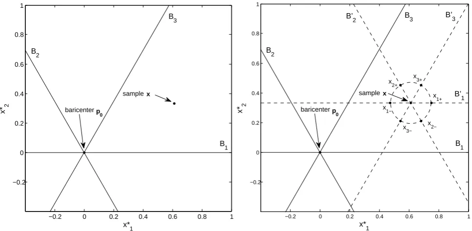
The texture of a soil sample x=(C, Z, L) is defined by the distribution of the soil particle sizes C (clay, diame-ter<2 µm),Z (sand, diameter>2 mm) andL(silt, 2 µm< diameter<2 mm). Because the parts cannot vary indepen-dently (there are only two degrees of freedom), it is possi-ble to visualise the soil texture, a 3-D composition, in two dimensions by means of an equivalent representation in the texture triangle (Fig. 1). This is an equilateral triangle with vertices atp1= (100, 0, 0), p2= (0, 100, 0) andp3= (0, 0, 100). The three vertices are defined counter-clockwise and are connected through the segmentsp1p3,p3p2andp2p1, scaled from 0 to 100.

In the texture triangle, three bisectors are defined as the straight lines through one of the vertices and the barycen-terp0=

100 3 ,

100 3 ,

100 3

(see Fig. 1). The bisector through vertexp1,p2andp3is referred to as B1, B2, and B3, respec-tively, and has the property that the values of two parts of the composition are always equal on this line.

2.3 Local sensitivity analysis on compositional data

The aim of a local sensitivity analysis is to measure the effect of perturbing a specific compositionx, i.e. inducing small relative changes to the composition, on the model out-put y. The sensitivity of y with respect tox is expressed as a sensitivity function that is defined as the derivative of y with respect tox and is evaluated at one particular value ofxby using the finite difference approximation. Therefore, small changes inxneed to be imposed that, considering the closed character ofx, imply a change in each of its partsxi

(i=1,2, ..., D)while maintainingPD

i=1xi =κ. The model 0

20 40

60 80

0 20

40 60

80

0

20

40

60

80

Sand [%] Clay [%]

Silt [%]

B

3

100

B

1

B

2

x

baricenter

p 2

100

p 3 p

1

100

sample

p 0

area where Rawls and Brakensiek [1985,1989] PTFs are valid

x 2=Z x

1=C

x 3=L

Fig. 1.Representation of a samplex= (C,Z,L)in the texture triangle with indication of the bisectorsB1,

B2andB3, the verticesp1,p2,p3and the boundary conditions on the PTFs of Rawls and Brakensiek (1985,

1989).

26

Fig. 1. Representation of a samplex=(C, Z, L)in the texture tri-angle with indication of the bisectors B1, B2and B3, the vertices

p₁,p₂,p₃and the boundary conditions on the PTFs of Rawls and Brakensiek (1985, 1989).

output y is said to be sensitive to model input x if small changes inx produce large changes iny. On the contrary, yis called insensitive toxif small changes inxhave almost no effect ony.

2.3.1 Perturbing in the 2-D euclidean space

The methodology presented in this paper for perturbing compositional data is built by analogy with a perturba-tion in a two-dimensional Euclidean space. Suppose we want to simultaneously perturb two inputsx₁∗ andx₂∗ with a factor ξ, four possible outcomes are evident and are given by the Cartesian coordinates(x₁∗·(1+ξ ), x₂∗·(1+ξ )), (x₁∗ · (1 − ξ ), x₂∗ · (1 − ξ )),(x₁∗·(1+ξ ), x₂∗·(1−ξ )), (x₁∗·(1−ξ ), x₂∗·(1+ξ )). These are the intersections of the bisectors of the Cartesian coordinate system and the circle with centrex=(x₁∗, x₂∗)and radiusd=

q

(ξ x₁∗)2_{+(ξ x}∗

2)2. The circle defines all possible perturbations and is therefore further referred to as the perturbation circle. Since it is im-possible to evaluate an infinite number of perturbations, only a limited set of perturbed points, e.g. the four points on the bisectors, can be considered.

This idea is adopted for the perturbation of a 3-D com-positionx=(x1, x2, x3). Consider a random samplexfrom S3which is defined by its triangular coordinates in a ternary diagram (see Fig. 1). Through ILR transformation, the com-position can be represented in the 2-D Euclidean space by

means of the Cartesian coordinates (Fig. 2a):

x₁∗, x₂∗= √1

6ln x₁2 x2·x3

!

,√1

2ln

_x

2 x3

!

. (5)

Likewise, any geometric shape on the ternary diagram can be transformed. Figure 2a shows that after ILR transforma-tion, the bisectors B1, B2, and B3 preserve their angles of 60◦ (see Sect. 2.2.2) and the barycenter p0 forms the ori-gin of the Cartesian system in which the bisectors inter-sect. The perturbation of samplex with factor ξ can now be performed in the Euclidean space, following the method-ology described above. First of all, the perturbation circle with centrex=(x₁∗, x₂∗)and radiusd=

q

(ξ x₁∗)2_{+(ξ x}∗

2)2 is constructed (Fig. 2b). As only a perturbation in the direc-tions given by the bisectors (further called perturbation axes) is considered, the directions of the bisectors are transferred to compositionx by means of a translation. The perturbed points are then defined by the intersectionsxi+andxi−

be-tween the translated bisectors B0i (i∈ {1,2, .., D}) and the

perturbation circle (Fig. 2b). Finally, the Cartesian coordi-nates of the perturbed compositions xi+ andxi− are back

transformed to the simplex through an inverse ILR transfor-mation (Egozcue et al., 2003) (Fig. 3, see further).

2.3.2 Perturbing in the simplex

Yet, in order to avoid the roundabout method of coordinate transformations, the operations in the Euclidean space are mimicked by operations in the simplex. This results in the following procedure to perturb a compositionx with a con-stant factorξ:

1. Perform one of the scalar multiplicationsx±=(1±ξ )

x (Eq. 3) in order to rescale the compositionx with a factorξ. The scaling factorξ determines the magnitude of the perturbation, i.e. the higher the value ofξ, the more the perturbed composition will deviate from the sampled compositionx.

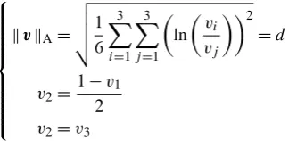
2. Calculate the Aitchison distancedA(x,x±) = d(Eq. 4)

in order to quantify the difference between the sampled compositionx and the rescaled compositionsx+ and

x−. Note that for the same value of ξ, the value of d

increases with increasing values ofkxk_A.

3. Define a circle with centrep0 and radiusd and deter-mine the intersections between the circle and the pertur-bation axes, here the bisectors B1, B2, and B3(Fig. 3). For each axis in directioni∈ {1,2, .., D}, this problem is solved by searching for the compositionsvi+andvi−

on the axis that satisfy the conditionkvikA=d(see Ap-pendix). The resulting compositions are further called directional vectors because they are necessary to trans-fer the direction of the perturbation axes to the sampled compositionx.

4. Add the directional vectors vi+ and vi− (i∈ {1,2, .., D}) to the compositionx (Eq. 2). This results in three pairs of new compositions{xi+,xi−}that lie

on the perturbation circle (Fig. 3). Since the performed operation preserves the distance in the simplex, the per-turbation circle aroundxhas radiusd. Although its cir-cular shape is distorted in the simplex (the further from the barycenter, the more distortion; examples of circles are shown in Fig. 3), the definition of a circle remains valid.

In summary, when perturbing compositionxin the simplex SD with a fixed factor ξ following the methodology de-scribed above, we obtain three pairs of new compositions

{xi+,xi−}withi∈ {1,2, .., D}that are a subset of all

pos-sible perturbations, defined by the circle with centrex and radiusd=dA(x,xi±). Note that althoughM∈Nother

per-turbation axes could have been chosen by selectingMpoints on a circle around the barycenter, either at random or such that they form angles of 360_2M degrees, and by connecting each of the selected points with the barycenter. In case ofM per-turbation axes, steps 4 and 5 from the methodology would re-spectively result inMpairs of directional vectors{vi+,vi−}

andM pairs of perturbed compositions{xi+,xi−}. In this

study, we selected the bisectors as perturbation axes (hence, M=3) such that the perturbed compositions (i) define an-gles of 60◦degrees on the perturbation circle, and (ii) lie on the translated bisectors B0_i, connectingxwith vertexp_i (see Fig. 3). The compositional lines B0_i also illustrate the effect of increasing (or decreasing) the magnitude of perturbation in directioni, as the perturbed compositions always lie on this line but shift towards (or away from) vertexpi.

Note that generalizing the methodology might raise some difficulties (Egozcue, 2012). ForM >3, calculating the di-rectional vectors in the ternary diagram becomes compli-cated. In this case, it is advised to rely on a simplicial ex-pression that computes the ILR coordinates of the directional vectors as the intersection points of the circle with radiusd and centerp0andMperturbation axes, regularly distributed on the circle. Through inverse ILR transformation, the direc-tional vectors are expressed in the simplex. ForD >3, e.g. when soil texture is described with more than three parts, the perturbation circle is not easily generalised to a sphere or hyper-sphere and the distribution of the perturbation axes might raise difficulties (Egozcue, 2012).

2.3.3 Calculating the sensitivity index

L. Loosvelt et al.: Sensitivity analysis for compositional data 467

−0.2 0 0.2 0.4 0.6 0.8 1

−0.2 0 0.2 0.4 0.6 0.8 1 x*₁ x* 2 B 2 B₃ B 1 baricenter p 0 sample x (a)

−0.2 0 0.2 0.4 0.6 0.8 1

−0.2 0 0.2 0.4 0.6 0.8 1 x* 1

x* 2 baricenter p

0

sample x

B 2

B’

2 B3 B’3

B’ 1 B₁ x 2+ x 3+ x 1+ x 2− x 3− x 1− (b)

Fig. 2. (a) Representation of the baricenterp0, the sampled compositionxand the bisectorsB1,B2andB3

after ILR transformation and (b) illustration of perturbation in the 2D Euclidean space with indication of the

perturbed compositions{xi+,xi−}and the translated bisectorsB01,B02andB03.

27

−0.2 0 0.2 0.4 0.6 0.8 1 −0.2 0 0.2 0.4 0.6 0.8 1 x*₁ x*2 B 2 B 3 B 1 baricenter p₀

sample x

(a)

−0.2 0 0.2 0.4 0.6 0.8 1

−0.2 0 0.2 0.4 0.6 0.8 1 x* 1

x* 2 baricenter p

0

sample x

B₂

B’₂ B₃ B’ 3 B’₁ B₁ x 2+ x 3+ x 1+ x 2− x 3− x 1− (b)

Fig. 2. (a) Representation of the baricenterp0, the sampled compositionxand the bisectorsB1,B2 andB3

after ILR transformation and (b) illustration of perturbation in the 2D Euclidean space with indication of the

perturbed compositions{xi+,xi−}and the translated bisectorsB01,B02andB03.

27

Fig. 2. (a) Representation of the barycenter p0, the sampled compositionx and the bisectors B1, B2 and B3after ILR transformation

and (b) illustration of perturbation in the 2-D Euclidean space with indication of the perturbed compositions{xi+, xi−}and the translated bisectors B0₁, B0₂and B0₃.

0 20 40 60 80 0 20 40 60 80 0 20 40 60 80 Sand [%] Clay [%] Silt [%] 100 100 p 1 p

2 p3

x 3− x1+ x2− x3+ x 1− x2+ sample x baricenter p 0 v 1+ v 3−

v2+ v1−

v 3+ v2− 100 B 2 B 3 B’ 3 B’ 2 B’

1 B1

Fig. 3. Perturbation in the simplex of a compositionxsampled from the texture triangle with indication of

the directional vectors{vi+,vi−}, the perturbed compositions{xi+,xi−}, the bisectorsB1,B2andB3and

the translated bisectorsB0

1,B02andB03; illustration of compositional circles at different locations in the texture

triangle.

28

Fig. 3. Perturbation in the simplex of a compositionx sampled from the texture triangle with indication of the directional vectors {vi+,vi−}, the perturbed compositions {xi+, xi−}, the bisectors B1, B2and B3and the translated bisectors B0₁, B0₂ and B0₃;

illus-tration of compositional circles at different locations in the texture triangle.

In the simplex, a compositionx is sampled uniformly at random from the sample space. Therefore, a Dirichlet distri-bution is defined, which is the multivariate generalisation of the beta distribution and is parametrized by a vectorα. The density function of the Dirichlet distribution is given by

fD(x;α)=

0PD i=1αi

5D_i=10(αi)

5D_i=1x_iαi−1 (6)

withx=(x1, ..., xD)a sample fromSD,α=(α1, ..., αD)the

parameter vector andDthe dimension of the sample space. In order to guarantee that the composition is sampled uni-formly at random, the condition α=1 should be fulfilled. The sampled composition x is thereupon perturbed in M different directions following the methodology described in Sect. 2.3.2.

After sampling and perturbing x, the model outputyt is determined at time stept for both the sampled composition xand the perturbed compositionsxi+andxi−. For each

di-rectionigiven by the perturbation axes, a forward and back-ward directional sensitivity function, respectively denoted as ∇_v

i+yt(x)and∇vi−yt(x), are calculated using the finite

difference technique:        ∇_v

i+yt(x)≈

yt(x⊕vi+)−yt(x) dA(x⊕vi+,x)

=yt(xi+)−yt(x)

d

∇_v

i−yt(x)≈

yt(x)−yt(x⊕vi−)

dA(x⊕vi−,x)

=yt(x)−yt(xi−)

d

(7)

witht the time step of model outputy,vi± the directional

vectors for perturbation in directioni andd the Aitchison distance (see Eq. 4). Averaging both functions leads to a cen-tral, directional sensitivity function∇_iyt(x), which indicates the average change iny caused by opposite changes inx in the direction of perturbation axisi:

∇_iyt(x)≈

yt(x⊕vi+)−yt(x⊕vi−)

dA(x⊕vi+,x⊕vi−)

=yt(xi+)−yt(xi−)

2D . (8)

As the sensitivity function itself is not useful for sensitivity analysis (Saltelli et al., 2008b), it is summarised into an om-nidirectional local sensitivity indexS (by analogy with the sensitivity index proposed by Hill and Tiedeman (2007)):

S(x)= 1

M

M

X

i=1

v u u t

1 N

N

X

t=1

(∇_iyt(x))2 (9)

withN the number of time steps in the model output and Mthe number of perturbation axes (hereM=3). The sen-sitivity index is hence a single value that reflects the average response ofywhenxis perturbed with a fixed factorξ inM different directions, each covering two opposite changes in x. It is calculated as the root mean squared difference in the model output resulting from two oppositely perturbed com-positions, averaged over the different perturbation directions. As such, the sensitivity index can be easily updated when

∇_iyt(x)is calculated for additional perturbation directions, i.e.M >3. In case the model outputyis time-independent, i.e.N=1, then S reduces to the mean absolute difference in the model output resulting from two oppositely perturbed compositions. An overview of the methodology to calculate the sensitivity index is given in Algorithm 1.

Note that for D >3, a large number of points on the perturbation (hyper-)sphere will be required to compute the sensitivity index. In this case, computation of the sensitiv-ity function can be simplified by estimating the directional derivatives based on the ILR coordinates of the sampled composition:

∇_v

iyt(x)=

_∂y

t

∂x₁∗, ∂yt ∂x₂∗, ...,

∂yt ∂x_D∗_-1

· v₁∗_,i, v∗_2,i, ..., v∗_D-1,i> (10) As such, any directional derivative can be computed if for each of theD-1 orthogonal axis on the ILR coordinate space, the gradient∂yt/∂x∗has been determined (Egozcue, 2012).

2.3.4 Optimizing the perturbation factor

The choice of the perturbation factorξdetermines the quality of the sensitivity function: the smaller its value, the better the

Algorithm 1: Calculate the local sensitivity indexS for a sampled compositionx

Data: - a compositionxfrom the sample spaceSD

(Sect. 2.3.2);

– a perturbation factorξ(Sect. 2.3.4); – a set ofMperturbation directions; Result: sensitivity indexSforyatx

begin

perform the scalar multiplication(1±ξ )x=x± (Sect. 2.3.2, step 1);

calculate the Aitchison distancedA(x,x±)(Sect. 2.3.2, step 2);

for each perturbation directioni∈ {1,2, .., M}do determine the directional vectors{vi+,vi−} (Sect. 2.3.2, step 3);

add the directional vectors toxto obtain{xi+,xi−} (Sect. 2.3.2, step 4);

apply the model to determineyt(xi+)andyt(xi−); approximate the central, directional sensitivity function∇_iyt(x)(Eq. 8)

calculate the omnidirectional local sensitivity indexS(x)

(Eq. 9) end

finite difference scheme approximates the derivative. How-ever, ifξ is taken too small it might give rise to numerical errors. If ξ is taken too large, errors due to model nonlin-earities might be introduced in the analysis (De Pauw and Vanrolleghem, 2006). Therefore, an optimization procedure is included in the presented SA framework. The basic idea is to make both types of error as small as possible by minimiz-ing the difference in model sensitivity when inducminimiz-ing oppo-site changes in the model input, i.e. the difference between the sensitivity functions∇_v

i+yt(x)and∇vi−yt(x)should be

as small as possible when perturbing in directioni. Although several measures can be used to quantify this difference, the sum of squared difference between their absolute values is selected in this study and is denoted asCi(x):

Ci(x)=

1 N

N

X

t=1

∇vi+yt(x)

−

∇vi−yt(x)

2

. (11)

By taking the absolute value of the sensitivity functions, we allow that opposite changes inx result in non-opposite, but similar model responses. Since the sensitivity analysis explores M directions on the perturbation circle, M val-ues ofCi(x)are obtained on which the minimization

pro-cedure needs to be carried out. In order to solve this opti-mization problem, the maximum value over allCi(x)(with

L. Loosvelt et al.: Sensitivity analysis for compositional data 469

Algorithm 2: Optimise the perturbation factor ξ for a sampled compositionx

Data: – a compositionxfrom the sample spaceSD

(Sect. 2.3.2);

– a set ofLperturbation factorsξ(Sect. 2.3.4); – a set ofMperturbation directions;

Result: optimal perturbation factorξatx

begin

apply the model to determineyt(x);

for eachξ∈ {ξ1, ξ2, .., ξL}do

perform the scalar multiplication(1±ξ )x=x± (Sect. 2.3.2, step 1);

calculate the Aitchison distancedA(x,x±) (Sect. 2.3.2, step 2);

for each perturbation directioni∈ {1,2, .., M}do determine the directional vectors{vi+,vi−} (Sect. 2.3.2, step 3);

add the directional vectors toxto obtain {xi+,xi−}(Sect. 2.3.2, step 4);

apply the model to determineyt(xi+)and

yt(xi−);

approximate the sensitivity functions∇_vi+yt(x)

and∇_v

i−yt(x)(Eq. 7);

calculateCi(x)(Eq. 11);

determineCmax(x)asmaxM

i=1Ci(x);

select the value ofξfor whichCmax(x)is minimal;

end

the methodology to optimise the perturbation factor for a sampled composition is given in Algorithm 2.

3 Results and discussion

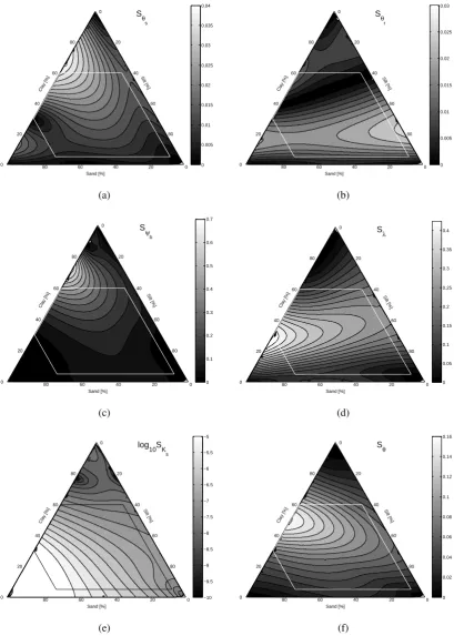
The experimental set-up consists of two main steps: in the first step, 100 textures are sampled from the texture triangle to determine the optimal factorξ for perturbing soil texture. In the second step, 5000 textures are sampled from the tex-ture triangle and are used as input to the hydrologic model to evaluate the response of the simulated soil moisture when texture is perturbed with the optimal perturbation factor.

3.1 Identification of the optimal perturbation factor

Hundred compositions are sampled from the texture trian-gle according to a Dirichlet distribution (with α=1). For each sampled texture, the perturbation factorξ is evaluated for the values in{10−5,10−4,10−3,10−2,10−1}by applying the methodology as described in Algorithm 2. For eachξ, we obtain 100 values ofCmaxof which the mean, the mini-mum and the maximini-mum are shown in Fig. 4b. The mean value ofCmaxclearly shows a minimum forξ=10−2, which sug-gests that this value is optimal for perturbing a broad range of textures. Although the minimum value ofCmaxis lowest

forξ=10−4_{, this perturbation factor can be discarded as} be-ing optimal since the spread over the different values ofCmax is very large for this value ofξ. Or stated differently: when ξ=10−4would be selected as optimal, it would result in a very low value ofCmaxfor only a limited number of textures, whereas the majority of the samples would be characterised by a larger value ofCmax. These findings are in correspon-dence with the frequency distribution of the optimalξ-values (Fig. 4b), which shows that for the major part (about 65 %) of the samples,Cmaxis minimal when they are perturbed with 10−2. For 25 % and 10 % of the samples, the optimal value of ξ is respectively smaller and larger than 10−2. The samples from the group with an optimal ξ smaller than 10−2 show a relatively heterogeneous distribution in the texture triangle (see Fig. 5) with the highest concentration around textures with a clay content above 40 % or a sand content between 20 % and 50 %. The samples from the group with an optimal ξ larger than 10−2_{are mainly located around textures with a} sand and clay content of 30 %.

For practical purposes, it is chosen to use a fixed value of 10−2for the perturbation factor, as it would unnecessar-ily increase the complexity of the sensitivity analysis when makingξ dependent of the sampled texture. Consequently, deviations from the optimal value are mainly located within the texture classes clay loam and loam (Fig. 5).

3.2 Identification of sensitive regions in the texture triangle

Identifying sensitive regions in the texture triangle with re-spect to the estimation of soil parameters or with rere-spect to the prediction of soil moisture is useful for the model user as it allows to reduce the uncertainty in the predicted variable. Since standardly available soil information is often limited to a soil map of the study area and a number of sparsely dis-tributed soil texture measurements, the measurement is as-sumed to be representative for the corresponding soil map unit. Consequently, the model user attributes the same parti-cle size distribution to all locations falling into that soil map unit, whereas the soil texture at a location different from the measurement point, but within the same soil map unit, may (largely) deviate from the sampled texture. Although it is as-sumed that the spatial variability within a homogeneous soil map unit covers only a minor part of the total variability in texture that is enclosed within the definition of the cor-responding soil type, the discrepancy between the scale of measurement and the scale of model application might in-troduce large uncertainties in the model output. If large un-certainties in either the estimated SHPs or the simulated soil moisture are not acceptable (depending on the objective of the study), the uncertainty about the potential bias in the mea-sured soil texture due to spatial variability should be further reduced through additional data collection. If the pattern in sensitivity is identified, the following rule of thumb to priori-tize additional data collection can be applied: “If the sampled

470 L. Loosvelt et al.: Sensitivity analysis for compositional data

−5E −4E −3E −2E −1E

10−10 10−8 10−6 10−4 10−2 100 102 104

Perturbation factor ξ Cm

a

x

(a)

−5E −4E −3E −2E −1E 0

10 20 30 40 50 60 70

Perturbation factor ξ

Frequency of samples

(b)

Fig. 4. The mean (full line), minimum and maximum (dotted lines) values ofCmax as a function of the

perturbation factorξ(a) and the frequency distribution of the optimal perturbation factor (b), for 100 sampled

compositions.

29

−5E −4E −3E −2E −1E

10−10 10−8 10−6 10−4 10−2 100 102

Perturbation factor ξ Cm

a

x

(a)

−5E −4E −3E −2E −1E

0 10 20 30 40 50 60 70

Perturbation factor ξ

Frequency of samples

(b)

Fig. 4. The mean (full line), minimum and maximum (dotted lines) values ofCmax as a function of the

perturbation factorξ(a) and the frequency distribution of the optimal perturbation factor (b), for 100 sampled

compositions.

29

Fig. 4. The mean (full line), minimum and maximum (dotted lines) values ofCmaxas a function of the perturbation factorξ (a) and the

frequency distribution of the optimal perturbation factor (b), for 100 sampled compositions.

(a)

0 20

40 60

80 100

Clay [%]

0 20

40 60

80 100

Sand [%] 0

20

40

60

80

100 Silt [%]

Sand Loamy Sand

Sandy Loam

Loam

Silt Loam

Silt Silty Clay

Loam Clay Loam

Sandy Clay Loam

Sandy Clay

Clay

Silty Clay

(b)

Fig. 5.Distribution of the optimal perturbation factorξ(100 samples) in the texture triangle (a) with

identifica-tion of the USDA soil classes (b).

(a)

0 20

40 60

80 100

Clay [%]

0 20

40 60

80 100

Sand [%] 0

20

40

60

80

100 Silt [%]

Sand Loamy Sand

Sandy Loam

Loam

Silt Loam

Silt Silty Clay Loam Clay Loam

Sandy Clay Loam

Sandy Clay

Clay

Silty Clay

(b)

Fig. 5.Distribution of the optimal perturbation factorξ(100 samples) in the texture triangle (a) with

identifica-tion of the USDA soil classes (b).

30

Fig. 5. Distribution of the optimal perturbation factorξ (100 samples) in the texture triangle (a) with identification of the USDA soil classes (b).

texture, which is assumed to be representative for a certain soil map unit, is located within a region of high sensitivity in the texture triangle, then additional texture samples within the area corresponding to this soil map unit, as delineated on the soil map, should be taken”. By accounting for the spa-tial variability, a more accurate estimate of the representative (most probable) texture for the given soil map unit can be formulated and can be used to reduce the uncertainty in the model output. On the contrary, if the sampled texture is lo-cated within a region of low sensitivity in the texture triangle, the discrepancy between the scale of measurement and the scale of model application will have a low impact on the pre-dicted variable, and taking additional samples may therefore

be discarded, unless a high spatial variability in soil texture exists.

3.2.1 Sensitivity of soil hydraulic parameters

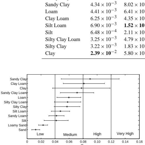
Five thousand compositionsT =(C, Z, L)are sampled from the texture triangle according to a Dirichlet distribution (with α=1) and are perturbed withξ=10−2. For both the sam-pled and perturbed compositions, the corresponding SHPs are estimated with the PTFs of Rawls and Brakensiek (1985), on which the sensitivity function∇_iSHP(T)withi∈ {1,2,3}

and the sensitivity indicesSSHP are calculated by applying the methodology as described in Algorithm 1. A contour plot

L. Loosvelt et al.: Sensitivity analysis for compositional data 471

ofSSHP(Fig. 6a–e) reveals that the sensitivity pattern highly depends on the parameter under consideration, although the patterns inSθs andSψb show a remarkable resemblance. For

these parameters, the hot spot of high sensitivity is located around textures with a clay content of 60–80 % and a sand content of 20–40 %. The sensitivitiesSθrandSλshow a

pat-tern that is highly dominated by the clay content: an increase in the clay content causes an increase (decrease) in the sen-sitivity if the clay content is lower (higher) than 30 %. Al-though the clay content of the hot spot matches forSθr and

Sλ, the corresponding sand content is different: around 0 %

for the former and around 70 % for the latter. On the con-trary, the pattern inSKsis dominated by the sand content: the

higher the sand content, the higher the sensitivity. The order of magnitude of the sensitivity index should be interpreted with respect to the corresponding SHP. Therefore, the mean predicted SHP over the entire texture triangle is given as a reference in Fig. 6. Also note that results outside the valid-ity zone of the PTFs should be interpreted with care (see Sect. 2.1.1 and Fig. 1). This zone is indicated on the con-tour plots in Fig. 6. In summary, the potential uncertainty in the predicted SHPs due to the discrepancy in scale between measurement and model application highly varies across the texture triangle and among the different SHPs, making it very difficult to formulate general guidelines to reduce the uncer-tainty in the predicted SHPs.

3.2.2 Sensitivity of soil moisture

After determining the sensitivity of the estimated SHPs to soil texture, the SHPs are used as input to the hydrologic model TOPLATS (run in spatially distributed mode) in or-der to simulate the daily soil moisture contentθtduring the year 2006 at the simulation location (see Sect. 2.1.2) under Belgian weather conditions (see Sect. 2.1.2). The 5000 sam-pled textures and their perturbed textures are successively at-tributed to the simulation location on which the correspond-ing sensitivity functions∇_iθt(T)withi∈ {1,2,3}and sen-sitivity indexSθ are calculated as described in Algorithm 1.

Figure 6f shows a contour plot ofSθ as a function ofT and

reveals a rather simple sensitivity pattern. For textures with a clay content lower than 35 % or higher than 70 %, the sen-sitivity is strongly determined by the clay content. In case C <35 %, the textural sensitivity increases with increasing values of the clay content, whereas in caseC >70 % the tex-tural sensitivity decreases with increasing values of the clay content. For soils with a clay content between 35 % and 70 %, Sθ is also highly influenced by the percentage of sand in the

soil. The hot spot of high sensitivity is located around tex-tures with a clay and sand content of 55 % and 45 %, respec-tively. This means that for these measured textures, the po-tential uncertainty inθ that is associated with the scaling is-sue will be the highest, but can, however, be reduced through additional data collection.

3.2.3 Evaluation of the USDA class as sensitivity region

The objective of this section is to investigate whether a soil map of a region with indication of the USDA soil classes can be used as a rudimentary tool to set up the texture sampling strategy prior to data collection. As such, the discrepancy be-tween the scale of measurement and the scale of model appli-cation within that region is optimally managed with respect to the uncertainty in the model prediction. For the predic-tion in a region that goes together with an USDA soil class that is attributed a high sensitivity towards soil texture, it is important to reduce the uncertainty on the textural variabil-ity within that region. Obviously, sufficient samples should be taken to accurately estimate the representative texture. By using the representative texture, a lower model prediction un-certainty is achieved. Otherwise, if the soil map indicates that the prediction will take place in a region where the soil class shows a low sensitivity towards texture, then resources can be saved and data collection can be limited to a single soil sam-ple. However, this strategy is only valid under the assumption that the textural variability within that region is low.

In order to associate regions of high and low sensitivity of the SHP estimation with the commonly used USDA soil clas-sification,SSHPis averaged over the samples falling into the same USDA soil class, further denoted asSSHP(Table 2). For θsandψb, the soil class corresponding to the highestSSHPis

clay, whereas forθr,λandKs this is respectively silt loam,

sandy clay loam and sandy loam, which are also the classes

that contain the hot spot of high sensitivity for their respec-tive SHP (Fig. 6). However, the hot spot only covers a part of the entire soil class, such that advising a higher sampling density to formulate a representative texture for the corre-sponding soil map units will not always be relevant. Based on these results, we may argue that the USDA classification is only useful as a preliminary indication for the sensitivity in SHP prediction because the variation in sensitivity within an USDA class is often high. As a consequence, the USDA soil map is suboptimal when used as a tool to optimise the sampling strategy with respect to the potential uncertainty in the estimated SHPs that is associated with the scaling is-sue. These findings call for a refinement of the USDA soil classes as they seem to be too rough to accurately describe the soil texture. In addition, the definition of soil texture should evolve towards a representation with more than three grain classes.

By analogy,Sθ is averaged over each USDA soil class and

the resultingSθ is shown together with its standard

devia-tion in Fig. 7. Based on the total range inSθ, four sensitivity

classes are defined: low sensitivity (0≤Sθ <0.04), medium

sensitivity (0.04≤Sθ<0.08), high sensitivity (0.08≤Sθ <

0.12) and very high sensitivity (0.12≤Sθ). The soil class

sandy clay is attributed the highestSθ and falls into the high

sensitivity class, which is obvious as this class contains the hot spot of high sensitivity (see Fig. 6). However, the vari-ation in sensitivity within that soil class is very large and

0 20

40 60

80

0 20 40 60 80

0

20

40

60

80

Sand [%]

Clay [%]

Silt [%]

0 0.005 0.01 0.015 0.02 0.025 0.03 0.035 0.04

S_θ

s

(a)

0 20

40 60

80

0 20 40 60 80

0

20

40

60

80

Sand [%]

Clay [%]

Silt [%]

0 0.005 0.01 0.015 0.02 0.025 0.03

S_θ

r

(b)

0 20

40 60

80

0 20 40 60 80

0

20

40

60

80

Sand [%]

Clay [%]

Silt [%]

0 0.1 0.2 0.3 0.4 0.5 0.6 0.7

S_ψ

b

(c)

0 20

40 60

80

0 20 40 60 80

0

20

40

60

80

Sand [%]

Clay [%]

Silt [%]

0 0.05 0.1 0.15 0.2 0.25 0.3 0.35 0.4

S_λ

(d)

0 20

40 60

80

0 20 40 60 80

0

20

40

60

80

Sand [%]

Clay [%]

Silt [%]

−10 −9.5 −9 −8.5 −8 −7.5 −7 −6.5 −6 −5.5 −5

log₁₀S_K

s

(e)

0 20

40 60

80

0 20 40 60 80

0

20

40

60

80

Sand [%]

Clay [%]

Silt [%]

0 0.02 0.04 0.06 0.08 0.1 0.12 0.14 0.16

S_θ

(f)

Fig. 6.

Contour plot of the sensitivity index across the texture triangle for the estimated soil hydraulic parameters

(a)-(e)

θ

(mean is 0.18

m

·

m

),

θ

(mean is 0.03

m

·

m

),

ψ

(0.16

m

),

λ

(mean is 0.49), and

log

K

(mean is

−

6

.

11m

·

s

) and for the simulated soil moisture content

θ

(f). Results outside the validity zone of

the PTFs (indicated by a white line) and near the borders of the triangle should be interpreted with care.

Fig. 6. Contour plot of the sensitivity index across the texture triangle for the estimated soil hydraulic parameters (a–e)θs (mean is

0.18 m3m−3),θr(mean is 0.03 m3m−3),ψb(0.16 m),λ(mean is 0.49), and log10Ks (mean is−6.11 m s−1) and for the simulated soil

moisture contentθ(f). Results outside the validity zone of the PTFs (indicated by a white line) and near the borders of the triangle should be interpreted with care.

L. Loosvelt et al.: Sensitivity analysis for compositional data 473

Table 2. Average sensitivity index within the USDA soil classes, for the different soil hydraulic parameters; the class with the highest average sensitivity is indicated in boldface, whereas the class with the lowest average sensitivity is in italics.

Soil Class Sθs Sθr Sψb Sλ SKs

Sand 5.84×10−4 5.02×10−4 5.02×10−4 7.21×10−3 1.77×10−6 Loamy Sand 1.33×10−3 1.44×10−3 2.24×10−3 2.04×10−2 4.84×10−6 Sandy Loam 4.72×10−3 8.12×10−3 2.55×10−2 1.09×10−1 1.07×10−5 Sandy Clay Loam 4.10×10−3 5.33×10−3 2.85×10−2 1.47×10−1 5.02×10−6 Sandy Clay 4.34×10−3 8.02×10−4 3.35×10−2 5.72×10−2 3.77×10−7 Loam 4.41×10−3 6.41×10−3 3.37×10−2 7.31×10−2 7.89×10−7 Clay Loam 6.25×10−3 4.35×10−3 5.07×10−2 1.00×10−1 2.38×10−7 Silt Loam 6.90×10−3 1.52×10−2 5.95×10−2 1.02×10−1 5.97×10−7 Silt 6.48×10−4 2.11×10−3 6.91×10−3 6.26×10−3 2.52×10−8 Silty Clay Loam 3.25×10−3 4.79×10−3 2.18×10−2 6.40×10−2 4.46×10−8 Silty Clay 3.22×10−3 1.83×10−3 2.62×10−2 5.39×10−2 1.91×10−8

Clay 2.39×10−2 5.80×10−3 2.61×10−1 1.49×10−1 9.45×10−8

Sandy Clay Clay Loam Clay Sandy Clay Loam Loam Silty Clay Loam Silty Clay Silt Loam Sandy Loam Silt Loamy Sand Sand

0 0.02 0.04 0.06 0.08 0.10 0.12 0.14 0.16 S_θ

Very High High

Medium Low

Fig. 7. Average sensitivity indexSθfor the 12 USDA soil classes with indication of the standard deviation

and the sensitivity classes low (0≤Sθ<0.04), medium (0.04≤Sθ<0.08), high (0.08≤Sθ<0.12) and very

high (0.12≤Sθ).

32

Fig. 7. Average sensitivity indexSθ for the 12 USDA soil classes

with indication of the standard deviation and the sensitivity classes low (0≤Sθ<0.04), medium (0.04≤Sθ<0.08), high (0.08≤

Sθ<0.12) and very high (0.12≤Sθ).

ranges from medium to very high. Also other soil classes enclose more than one sensitivity class, e.g. clay and silt, which would require to re(de)fine those soil classes with re-spect to their sensitivity. On the contrary, some USDA classes completely fall within a single sensitivity class. The classes

loamy sand and sand therefore correctly represent a low

sen-sitivity, whereas the classes loam, silty clay loam and silty

clay represent a medium sensitivity. This supports the

ear-lier findings to use the USDA soil classification (and hence the USDA soil map) only as a preliminary indication of the model output sensitivity towards textural changes. The dom-inant sensitivity class that is associated with the USDA class is then an indication of the sampling density needed to for-mulate a representative texture for the given USDA class. For example the clayey soil classes (e.g. sandy clay, clay loam and clay) will require a higher sampling density.

3.3 Identification of the hydrologic model behaviour

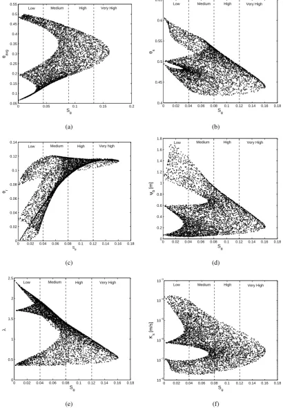
The scatterplot in Fig. 8a shows how the model response Sθ is related to the average annual soil moisture content

θavg=_N1 PNt=1θt simulated with TOPLATS, from which it is clear that very high model sensitivities are only expected if the simulated soil moisture has a value between 0.2 and 0.4, with a maximum around 0.3. On the contrary, low sen-sitivities occur for both very low (θavg<0.2) and very high soil moisture contents (θavg>0.45). This suggests that the more extreme (dry or wet) the soil moisture content becomes, the less uncertainty in the simulation result is involved when there is a discrepancy between the scale of texture measure-ment and the scale of model application. Similarly, scatter-plots betweenSθand the SHPs (Fig. 8b–f) reveal that the

sen-sitivity can only be very high if the SHPs take specific values: θs,θr,ψb,λandKsshould be within the range[0.42,0.49],

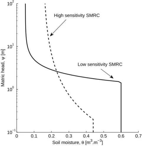
[0.1,0.12],[0.05,0.6],[0.4,1]and[5×10−8,5×10−6], re-spectively. The parameter values for which a maximum in Sθ is recorded, are combined to construct the SMRC that

in-volves the highest uncertainty inθ. The so-called “high sen-sitivity” SMRC shows a rather linear behaviour (Fig. 9) that is characteristic for fine-textured soils with a low effective porosity, i.e.θs−θr. For the sake of simplicity, it can be said that this SMRC corresponds to low values ofθs,ψbandλ, and a high value ofθr. On the contrary, a low sensitivity of the simulated soil moisture is not exclusively related to spe-cific values of the SHPs, since for a broad range of SHP val-ues the correspondingSθ falls into the low sensitivity class.

Nevertheless, it is observed that the more the SHP values de-viate from the specified range that gives rise to a very high sensitivity,Sθ shifts towards the low sensitivity class. This

means that the sensitivity of the simulated soil moisture is certainly low in caseθs,ψb andλhave a high value andθr has a low value. The so-called “low sensitivity” SMRC that results from this soil parameter combination is characteristic

0 0.05 0.1 0.15 0.2 0.05

0.1 0.15 0.2 0.25 0.3 0.35 0.4 0.45 0.5 0.55

θavg

S

θ

Low Medium High Very High

(a)

0 0.02 0.04 0.06 0.08 0.1 0.12 0.14 0.16 0.18 0.4

0.45 0.5 0.55 0.6 0.65

θs

S_θ

Low Medium High Very High

(b)

0 0.02 0.04 0.06 0.08 0.1 0.12 0.14 0.16 0.18

0 0.02 0.04 0.06 0.08 0.1 0.12 0.14

θr

S θ

Low Medium High Very high

(c)

0 0.02 0.04 0.06 0.08 0.1 0.12 0.14 0.16 0.18 0

0.2 0.4 0.6 0.8 1 1.2 1.4 1.6 1.8

ψb

[m]

S_θ

Low Medium High Very High

(d)

0 0.02 0.04 0.06 0.08 0.1 0.12 0.14 0.16 0.18 0

0.5 1 1.5 2 2.5

λ

S_θ

Low Medium High Very High

(e)

0 0.02 0.04 0.06 0.08 0.1 0.12 0.14 0.16 0.18

10−8

10−7

10−6

10−5

10−4

10−3

Ks

[m/s]

S_θ

Low Medium High Very High

(f)

Fig. 8.

Scatterplot between

S

and the soil hydraulic parameters

θ

,

θ

,

ψ

,

λ,

K

(a)-(e) and the average

simulated soil moisture content

θ

(5000 sampled textures).

Fig. 8. Scatterplot betweenSθ and the soil hydraulic parametersθs,θr,ψb,λ,Ks(a–e) and the average simulated soil moisture contentθavg

(5000 sampled textures).

L. Loosvelt et al.: Sensitivity analysis for compositional data 475

0 0.1 0.2 0.3 0.4 0.5 0.6 0.7 10−1

100 101 102

Soil moisture, θ [m3.m−3]

Matric head,

ψ

[m]

High sensitivity SMRC

Low sensitivity SMRC

Fig. 9.Soil moisture retention curve (SMRC) for which the sensitivity of the simulated soil moisture to textural

changes is the highest and the lowest, respectively.

34

Fig. 9. Soil moisture retention curve (SMRC) for which the sensitiv-ity of the simulated soil moisture to textural changes is the highest and the lowest, respectively.

for coarse-textured soils with a high effective porosity and shows a highly nonlinear behaviour.

4 Conclusions

Considering the omnipresence of compositional data in the geosciences, we developed a method to perform a local sen-sitivity analysis on compositional model inputs. As the dif-ferent parts of the input vary simultaneously, while preserv-ing the closed character of the input, this method allows to abandon incorrect practice of OAT-SA. In the presented SA method, a sensitivity index is calculated based on the finite difference technique to approximate the directional deriva-tives of the model output with respect to the compositional model input. Local perturbations of the compositions were realised by operations in the simplex (for complex SA prob-lems we suggest to implement the alternative approach using ILR coordinates) and we relied on the assumption that all possible perturbations are defined by a perturbation circle. Additionally, we supplemented the SA method with a proce-dure to optimise the perturbation factor in order to minimise numerical errors and errors due to model nonlinearities.

The SA method was subsequently applied to a hydrologic model to assess the sensitivity of the simulated soil moisture content to changes in soil texture, for a high number of com-positions in the texture triangle. In a first step, we found that the optimal factor to perturb soil texture is 10−2. Although this value was found to be optimal in 65 % of the cases, it was

chosen to use a fixed value ofξ in order not to unnecessar-ily complicate the sensitivity analysis. However, one should be aware that in 10 % of the cases this value is too low and might introduce numerical errors in the sensitivity analysis, and that in 25 % of the cases this value is too high, which might result in errors due to the nonlinear behaviour of the hydrologic model. Especially near the borders of the ternary diagram, deviation of the perturbation factor from its opti-mal value might affect the sensitivity analysis. A perturbation factor of 10−2was used to perform a local SA on 5000 dif-ferent textures, sampled according to a Dirichlet distribution from the texture triangle. The analysed models are the PTFs of Rawls and Brakensiek (1985) and the hydrologic model TOPLATS of which the generated outputs are respectively the soil hydraulic parameters and the soil moisture content. Based on these model applications, the sensitivity index was calculated for both model outputs and was evaluated with respect to the position of the sampled texture in the texture triangle.

The results of the sensitivity analysis were found to be use-ful (i) to reduce the uncertainty on the modelled output when there is a discrepancy between the scale of measurement and the scale of model application and (ii) to gain more insight into the behaviour of the applied model, and more specifi-cally on how it reacts on changes in the soil texture with re-spect to its position in the texture triangle. As such, we found that the simulated soil moisture is most sensitive to soil tex-ture when the measured clay content is around 55% and the sand content around 45 %. This means that the potential un-certainty that is involved with the scaling issue will be the highest under these textural conditions. Therefore, when high uncertainties in the modelled output are not acceptable, it is advised to take one or more additional texture samples within the soil map unit that encloses the original sample such that a better estimate of the most probable texture can be formu-lated. Similarly, we identified zones of high sensitivity for the soil parameters, showing a high variability in their sensitivity pattern. We also investigated whether a soil map with indica-tion of the USDA soil classes can be used as a tool to opti-mise the texture sampling strategy by reviewing the USDA soil classification with respect to the pattern in model output sensitivity. The results point out that USDA classes are only useful as a rudimentary indication for the sensitivity as they distinguish between high and low sensitivity, but comprise a large within-class-variability of the sensitivity. Especially the clayey soil classes sandy clay, clay loam and clay involve high to very high sensitivities, such that it is advised to ap-ply a high(er) sampling density within these soil map units to calculate the representative texture. Furthermore, we were able to relateSθ to the shape of the soil moisture retention

curve and recorded the highest sensitivity when the values of θs,ψbandλare low and the value ofθris high. The result-ing curve is characteristic for fine-textured soils with a low effective porosity and shows a rather linear behaviour.