Inference of Non-Overlapping Camera Network Topology using Statistical Approaches

University of Windsor University of Windsor

Scholarship at UWindsor

Scholarship at UWindsor

Electronic Theses and Dissertations Theses, Dissertations, and Major Papers

2011

Inference of Non-Overlapping Camera Network Topology using

Inference of Non-Overlapping Camera Network Topology using

Statistical Approaches

Statistical Approaches

Abedalrhman Alkhateeb

University of Windsor

Follow this and additional works at: https://scholar.uwindsor.ca/etd

Recommended Citation Recommended Citation

Alkhateeb, Abedalrhman, "Inference of Non-Overlapping Camera Network Topology using Statistical Approaches" (2011). Electronic Theses and Dissertations. 312.

https://scholar.uwindsor.ca/etd/312

This online database contains the full-text of PhD dissertations and Masters’ theses of University of Windsor students from 1954 forward. These documents are made available for personal study and research purposes only, in accordance with the Canadian Copyright Act and the Creative Commons license—CC BY-NC-ND (Attribution, Non-Commercial, No Derivative Works). Under this license, works must always be attributed to the copyright holder (original author), cannot be used for any commercial purposes, and may not be altered. Any other use would require the permission of the copyright holder. Students may inquire about withdrawing their dissertation and/or thesis from this database. For additional inquiries, please contact the repository administrator via email

Inference of Non-Overlapping Camera Network Topology

using Statistical Approaches

by

Abedalrhman Alkhateeb

A Thesis

Submitted to the Faculty of Graduate Studies through Computer Science

in Partial Fulfillment of the Requirements for the Degree of Master of Science at the

University of Windsor

Windsor, Ontario, Canada

2011

© 2011 Abedalrhman Alkhateeb

Inference of Non-Overlapping Camera Network Topology

using Statistical Approaches

by

Abedalrhman Alkhateeb

APPROVED BY:

_________________________________ Dr. Faouzi Ghrib

Department of Civil and Environmental Engineering

______________________________________________ Dr. Imran Ahmad

School of Computer Science

______________________________________________ Dr. Boubaker Boufama, Advisor

School of Computer Science

______________________________________________ Dr. Ziad Kobti, Chair of Defense

DECLARATION OF ORIGINALITY

I hereby certify that I am the sole author of this thesis and that no part of this thesis has

been published or submitted for publication.

I certify that, to the best of my knowledge, my thesis does not infringe upon anyone’s

copyright nor violate any proprietary rights and that any ideas, techniques, quotations, or

any other material from the work of other people included in my thesis, published or

otherwise, are fully acknowledged in accordance with the standard referencing practices.

Furthermore, to the extent that I have included copyrighted material that surpasses the

bounds of fair dealing within the meaning of the Canada Copyright Act, I certify that I

have obtained a written permission from the copyright owner(s) to include such

material(s) in my thesis and have included copies of such copyright clearances to my

appendix.

I declare that this is a true copy of my thesis, including any final revisions, as approved

by my thesis committee and the Graduate Studies office, and that this thesis has not been

submitted for a higher degree to any other University or Institution.

iv ABSTRACT

This work proposes an unsupervised learning model to infer the topological

information of a camera network automatically. This algorithm works on non-overlapped

and overlapped cameras field of views (FOVs). The constructed model detects the

entry/exit zones of the moving objects across the cameras FOVs using the

Data-Spectroscopic method.

The probabilistic relationships between each pair of entry/exit zones are learnt to

cover the topological information among the different camera FOVs. Increase the

certainty of the probabilistic relationships using Computer-Generating to create more

Monte Carlo observations of entry/exit points. Our method requires no assumptions, such

as input parameters of the system, no processors for each camera and no communication

among the cameras. The purpose is to figure out the relationship between each pair of

linked cameras using the statistical approaches which help to track the moving objects

and predict the future location of them depending on their present location.

The Output is shown as a Markov chain model that represents the visible and

DEDICATION

ACKNOWLEDGEMENTS

All praise and glory to Almighty Allah (God) who gave me courage and patience

to carry out this work. Peace and blessing of Allah be upon my teacher Muhammad

(Peace Be upon Him)

For my parents the one who have struggled in their life to make my life easier,

thanks for the emotional and financial support you. May Allah reward you later on.

For my brother (Mohammad), the one I grow-up with, and share all childhood

memories with, thanks for all kind of support you gave me.

For my beloved wife (Crystalena), the one who stood up behind me in good and

bad, I really appreciate everything.

Especial thanks to Dr. B. Boufama my supervisor; I appreciate your

encouragement, advices and support. Finally thanks for the university of Windsor staff

Table of Contents

DECLARATION OF ORIGINALITY ... iii

ABSTRACT... iv

DEDICATION...v

ACKNOWLEDGEMENTS... vi

LIST OF TABLES... ix

LIST OF FIGURES...x

I. INTRODUCTION 1 1.1 COMPUTER VISION ... 1

1.2 HISTORY OF COMPUTER VISION ... 2

1.3 CAMERA NETWORK TOPOLOGY ... 3

1.4 APPLICATIONS OF LEARNING THE CAMERA NETWORK TOPOLOGY 4 1.5 MOTIVATION ... 5

1.6 OVERVIEW... 6

II. BACKGROUND OF CAMERA NETWORK TOPOLOGY 7 2.1 BASIC CAMERA (PINHOLE MODEL) ... 7

2.2 CAMERA FIELD OF VIEW (FOV)... 8

2.3 OBSERVATIONS DETECTION... 9

2.4 LEARNING ENTRY/EXIT ZONES... 10

2.5 BLOB CONSTRUCTION: ... 14

2.6 NOISE REDUCTION... 14

2.7 MARKOV CHAIN MONTE CARLO ... 16

III. RELATED WORK 19

IV. DESIGN AND METHODOLOGY 24

4.1 OBSERVATION DETECTION ... 25

4.2 LEARNING ENTRY/EXIT ZONES... 27

4.3 COMPUTER-GENERATING OBSERVATIONS AND OPTIMIZATION USING MONTE CARLO ... 29

4.4 DETECTING THE LINKS BETWEEN EACH PAIR OF ENTRY/EXIT ZONES ... 30

4.5 CALCULATING THE TRANSITION TIME FOR THE LINKED ENTRY/EXIT ZONES ... 32

4.6 THE OUTPUT ... 34

4.7 CONCLUSION ... 35

V. EXPERIMENTAL RESULTS 36 5.1 FOUR NETWORKED CAMERA ... 36

5.2 FIVE NETWORKED CAMERA ... 42

VI. CONCLUSIONS AND RECOMMENDATIONS 46 6.1 CONCLUSION ... 46

6.2 FUTURE WORK ... 47

REFERENCES...48

LIST OF TABLES

TABLE 2.1:SUMMARY OF OBSERVATIONS DETECTION APPROACH IS USED BY THE

RESEARCHERS. ... 10

TABLE 3.1:APPROACHES ARE USED FOR CAMERA NETWORK LOCALIZATION... 22

TABLE 4.1:SAMPLE OF DETECTED OBSERVATIONS... 25

TABLE 4.2:MONTE CARLO SIMULATION FOR GENERATING OBSERVATION... 30

TABLE 4.3:ALGORITHM FOR DETECTING THE LINKED ENTRY/EXIT ZONES... 31

TABLE 4.4:LEARNING THE RELATIONSHIP BETWEEN PAIR OF NETWORKED CAMERAS... 33

TABLE5.1:CLASSIFIED OBSERVATIONS FOR CAMERA 1 ... 38

TABLE 5.2:THE ADJACENCY MATRIX OF TRANSITION TIME... 41

TABLE 5.3:DETECTING THE OVERLAPPED CAMERAS FOVS IN THE CAMERA NETWORK... 41

LIST OF FIGURES

FIGURE 1.1: A)OVERLAPPED CAMERAS FOV B)NON-OVERLAPPED CAMERAS FOVS.. 3

FIGURE 2.1:CAMERA PINHOLE MODEL... 7

FIGURE 2.2:CAMERA INTRINSIC PARAMETERS... 8

FIGURE 2.3:CAMERA FIELD OF VIEW... 8

FIGURE 2.4: A)SPATIAL REPRESENTATION OF PATHS B):GRAPH REPRESENTATION OF PATHS... 11

FIGURE 2.5:SOURCES AND SINKS... 12

FIGURE 2.6:MOVING OBJECT IN CAMERA FOV ... 14

FIGURE 2.7: A)AN IMAGE OF SCENE HAS A VARIANT LIGHTENING... 15

B)THE IMAGE AFTER BACKGROUND SUBTRACTION, THE VARIATION OF LIGHT NOISE APPEARS AS A WHITE PIXEL... 15

FIGURE 2.8:MARKOV CHAIN MODEL... 17

FIGURE 3.1:SIMPLICIAL REPRESENTATION OF THE CAMERAS FOVS RELATIONS... 21

FIGURE 4.1THE PROPOSED MODEL FOR INFERENCE THE CAMERA NETWORK TOPOLOGY... 24

FIGURE 4.2: A)THE MOVING PERSON B)THE GRID OF THE 24 X 30 BOXES... 26

FIGURE 4.3:DETECTED OBSERVATIONS ENTRY/EXIT POINTS... 27

FIGURE 4.4: A)DASPEC CLUSTERS B)GENERAL K-MEANS CLUSTERS... 28

FIGURE 4.5: A)OVERLAPPED 2 CAMERAS FOV B)NON-OVERLAPPED 2 CAMERAS FOVS ... 33

FIGURE 4.6:MARKOV MODEL FOR NETWORKED CAMERA TOPOLOGY... 35

FIGURE 5.2:EXPERIMENT 1 CAMERA FOVS... 37

FIGURE 5.3:ALL CAMERAS OBSERVATIONS ARE CLUSTERED INTO MAIN ENTRY/EXIT ZONES ... 39

FIGURE 5.4:HISTOGRAM OF THE TRANSIT TIME OF THE OBSERVATIONS... 40

FIGURE 5.5:THE CAMERA NETWORK TOPOLOGY... 42

FIGURE 5.6:EXPERIMENT 2 SETUP... 43

FIGURE 5.7:EXPERIMENT 2 CAMERAS FOVS ... 44

CHAPTER I

INTRODUCTION

This chapter gives an overview of the general field of computer vision and the

topic of the thesis as well. A brief overview of computer vision and the historical

development of the field are discussed in the first two sections. Then camera network

topology is explained. After that, the main application of learning camera network

topology is described in general followed by the motivation of this work. Finally, the

chapter ends outlining the layout of the rest of this thesis.

1.1 Computer Vision

Computer vision is a mixed field of Artificial intelligence (AI); Image processing,

Computer graphic, Physics and Geometry fields. It is the computer science techniques

that are used to extract, recognize, classify and learn the information of computer images

in the real, 3D world.

Because the field is multidisciplinary, computer vision is a vast field and has

exchanged many visibility techniques with the related fields [Durand00]. Computer

vision is considered as a subfield of AI; many of the basic techniques were developed in

the AI laboratories. Computer vision and image processing have a significant overlap in

the basic techniques which have been developed in them. However, image processing

focuses more in image enhancement, image to image transformation and noise removal;

whereas computer vision focuses in 3D construction from one or several images.

Computer vision is the opposite of computer graphics since computer graphics generates

electromagnetic radiation using the image sensor [Ali06]. Computer vision is considered

as a subfield of the artificial intelligence - machine vision part, while machine vision

mainly focuses on the manufactory applications to control the robots. Computer vision

focuses more about the theoretical methods for these functions.

1.2 History of Computer Vision

During 1960’s digital image processing by computers started attracting

researchers. In 1965 the first computer vision system was built at MIT Lincolin

laboratory by L.G Robert [Kropatsch08]. A perspective view of a geometric model was

constructed on the computer; it was the first attempt to automatically recognize a 3D

object. Limitations of computer resources in those days motivated scientists to build

perceiving computers to handle the complex computer vision system [Kropatsch08]. The

needed resources where made available after a decade of work in the new computer

vision field. These new computers could process complicated mathematical applications

which were needed in order to further research in computer vision.

By the late 1970’s computer vision was considered as a discipline field [Ali06]. In

the early 1980’s [Delp82] stated that computer vision research in industrial robots was an

important field for the robotics industry. In 1987, the first international conference in

computer vision, ICCV, was held in London, UK [IEEE-ICCV]. Since the late 1980’s

research in human vision has increased; researchers started studying the human vision

functionality in which a discipline field is called neurobiology. This branch focuses on

1.3 Camera Network Topology

Camera network is an interdisciplinary area encompassing computer vision,

sensor networks, image, as well as signal processing [Zou09]. The network topology is

the layout pattern of interconnections of the various elements (links, nodes, etc.) of a

computer network [Learn-NT]. In video surveillance the camera network topology is the

layout pattern of the linked cameras; a pair of linked cameras has a path in which objects

can move through, or between them. The path can be a seen (i.e. corridor) or unseen path

(i.e. tunnel or hidden wall). Each camera in the network has a field of view (FOV), which

is the (angular or linear or area) extent of the observable world that is seen at any given

moment [Murray99]. If a pair of cameras fully or partially shares a field of view it means

they are overlapped, if not, it means they are non-overlapped cameras. Camera networks

differ depending on their cameras' FOVs. Some camera networks have only

non-overlapped FOVs cameras, some have only non-overlapped FOVs and the others have mixed

overlapped and non-overlapped FOVs cameras.

Figure 1.1: a) Overlapped cameras FOV b) Non-overlapped cameras FOVs

The network camera can be connected by wired or wireless communication. Due

development of wireless multimedia sensor networks, WMSNs, has advanced at great

speed [Akyildiz07]. Occasionally the networked cameras cannot be connected due to the

unavailability of the wireless or wired communication.

1.4 Applications of Learning the Camera Network Topology

1- People Tracking and Behaviour Interpretation

Topological information of the camera network can be used to anticipate the

future location of the target [Makris04]. The networked cameras collaborate to observe

the future location of the target [Funiak06]. Mapping the nodes in a camera network can

be an input parameter for different object tracking methods [Zou09], same as an agent’s

behaviour interpreting [Soro07].

2- Measuring Traffic Flow

Camera network localization can be used to analyze traffic flow and observe the

current transition time on a road. Camera network topology is used as a required

parameter of the smart traffic flow applications [Niu06].

3- Occlusion Handling in Video Surveillance

In video surveillance the object may hide behind another object, or in the blind

regions due to non-overlapped field of views. Learning about the spatial information of

the camera network can overcome the loss of the appearance information of the object

4- Event Detection

Much research has been focused on event detection, and activity analysis. The

applications of event detection range from simple motion detector [Nelson91] to

detecting aggressive behaviour (i.e. robbery at bank)[Zambanini09]. Spatial information

of the camera network can be useful for all kind of detection [Zou09].

5- Intelligent Environments

Intelligent environments are strongly influencing recent research in the computer

vision field. One of the most well-known applications is the smart home, which was

created to serve senior citizens and people with disabilities. Smart homes, combined the

fields of face recognition, object tracking and voice recognition to assist the target users

of these homes. Camera network localization is an essential requirement for this

application [Trivedi07].

1.5 Motivation

In the past twenty years the computer vision community has made great strides in

the automatic solutions to such problems as camera localization and visual tracking.

Camera based networks have been employed for critical real-time systems, such as

security monitoring and video surveillance. Researchers in this field focus on the smart

systems of automatic computer vision unsupervised learning methods. These can be set

These kinds of smart applications require the topological information of the

network’s cameras to determine the linked or the relative distance among them. Although

wireless communication has become available everywhere the communication among the

camera nodes in the network is still constrained by the bandwidth, data rate and energy.

Another important constraint is the limitation of the camera node processor as some

camera networks have basic video cameras, sensor, or low-level processing nodes.

Therefore, we do not make any assumption on the inputs from the camera network.

Our model input is simply a set of videos from one camera network. It does not

make any difference for us whether the cameras’ FOVs are overlapped or not, wired or

wireless, and whether or not they are connected. The output of our model is a graph

representing the relative location of each camera with respect to the other cameras in that

same network.

1.6 Overview

This thesis addresses the problem of learning the camera network topology that

has overlapped or non-overlapped camera field of views using the statistical information

of the moving objects through the cameras scenes. The thesis contains six chapters with

Chapter two explaining the background of the camera network topology and the

approaches that have been used to recover the topological information of the networked

cameras. Chapter three gives a brief overview of previous works in this area, while

Chapter four explains the approach we have used to recover the topology. The

experimental results are shown and analyzed in Chapter five. Finally, the conclusion and

CHAPTER II

BACKGROUND OF CAMERA NETWORK TOPOLOGY

This chapter gives the background of the camera network components and the

method used for creating these components. First, the basic units of the camera networks

are explained. Then the general methods for learning the camera network topology

processes are elaborated upon. Finally, the Markov chain Monte Carlo process is

discussed in general.

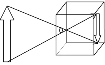
2.1 Basic Camera (Pinhole Model)

The pinhole camera is the most basic camera which consists essentially of a

light-proof, darkened box with a small hole in one side and no lens. When the photographer

takes a photo the light comes from the scene through the small hole, thus making the

scene appear upside down, and on the opposite side of the cameras hole. Alhassen (Ibn

Al-Haytham), a great authority on optics in the Middle-Ages who lived around 1000AD,

invented the first pinhole camera. The intrinsic parameters for this model includes the

focal length (ƒ), the principal point (p) and the skew coefficients, which is the angle

between x and y axis on the principle plane [Kamath07].

Figure 2.2: Camera Intrinsic Parameters

2.2 Camera Field of View (FOV)

The field of view, FOV, is the angular extent of the observable world that is seen

at any given moment. Different animals have different types of FOV, and humans have

an almost 180-degree forward-facing horizontal FOV. Camera FOV is the area of the

inspection captured on the camera’s imager. The size of the field of view and the size of

the camera’s imager directly affect the image resolution [Murray99].

2.3 Observations Detection

Observation detection is necessary for learning the camera network topology

without using wireless/wired connected camera nodes. Some models use the object

tracking approach to recover for camera network localization

[Meingast07][Lee00][Nam07][Marinakis05]. While others use the objects entry/exit

statistical information for camera network localizing [Tieu05][ Wang10][Makris04].

Most object tracking models use the spatio-temporal features for relating the object

trajectories.

Nam et al.[Nam07] proposed an original model for object tracking that establish

the object correspondence across the network’s cameras. A merged-spilt, MS, approach is

used for object occlusion which uses the grid-based approach for extracting the

appropriate spatio-temporal features. Chilgunde et al.[Chilgunde04] use the shape as a

feature-based object tracking for multi-camera network localization. They solved the

occlusion problem using the Kalman filter prediction. A colour histogram is used for

object tracking in the camera network localization model [Qurashi05]. The proposed

method used the HSV colour histogram to save many pictures for each pedestrian

crossing the road with different angles and sizes.

The bounding box feature-based tracking system is used to estimate the camera

network topology [Cralot09]. A bounding box made up of the lower left corner and the

upper right corner of the object’s blob. Wang et al. [Wang10] employ a correspondence

free model to classify the objects behaviours through studying the trajectories’ patterns in

each camera FOV. Boyd et al. [Boyed99] used the camera network topology for

statistically tracking the objects in the cameras’ FOVs by correlating the number of trips

statistical tracking approach, which is especially convenient for long term traffic patterns.

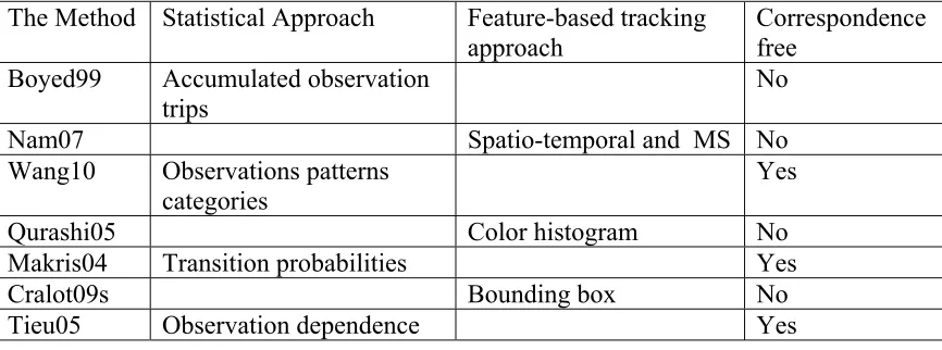
In Table 2.1, Observation detection models and approaches that were used by different

researchers are presented.

Table 2.1: Summary of observations detection approach is used by the researchers.

The Method Statistical Approach Feature-based tracking approach

Correspondence free

Boyed99 Accumulated observation trips

No

Nam07 Spatio-temporal and MS No

Wang10 Observations patterns

categories Yes

Qurashi05 Color histogram No

Makris04 Transition probabilities Yes

Cralot09s Bounding box No

Tieu05 Observation dependence Yes

From Table 2.1, one may notice that whenever the method is using a

feature-based object tracker the correspondence between object trajectories is required. On the

other hand, for statistical approaches there is no need for correspondence.

2.4 Learning Entry/Exit Zones

Learning entry/exit zones is very important for object tracking, object occlusion

and camera network localization systems. In [Makris02] an activity model is constructed

to identify the routes in an image. The proposed model is based on the recorded trajectory

observations by classifying them using a spatial feature, calculated using a simple

distance function. If an observation matches a learned route the function updates the

learned route with the new route weight information. Otherwise, the function creates a

The spatial model works on overlapped FOVs camera systems or a single camera

where pedestrians can be continuously tracked. However, it is inappropriate for

non-overlapped camera FOVs systems where tracked objects can be hidden in blind regions.

The clustering process is restricted by the object speed as the system cannot

recognize the object’s motion type. In other words, the system cannot distinguish

between a running, a walking or a lingering person in the scene. The system constructs

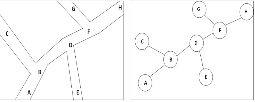
paths from the learned routes by grouping the connected routes and creating a junction

when the routes diverge in the cameras’ FOVs. The method reduces the number of

junctions by setting a threshold distance between each pair of routes before grouping or

creating a junction decision. Figure2.4 shows the spatial and graph representation of a

path; the alphabetical characters (A, B etc...) represent the junctions.

Figure 2.4: a) Spatial representation of paths b): Graph representation of paths

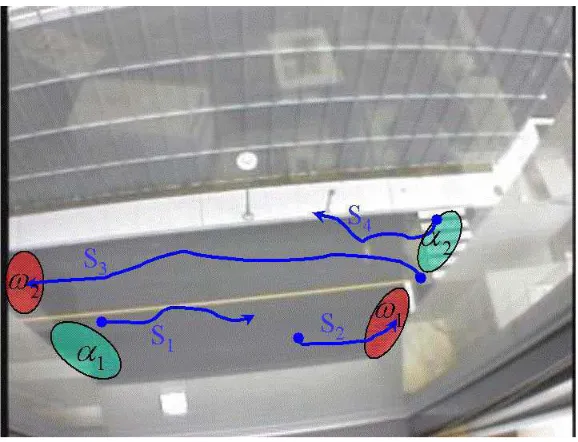
A method of fixing broken tracking sequences is introduced by stitching the

unlinked track scenes because of the “blind” areas while estimating source and sink

locations where objects appear in a camera FOV, and sink to locations where objects

disappear from a camera FOV (see Figure2.5). The standard Hungarian algorithm is used

for stitching the primary tracking correspondences resulting from the first model running

failure. The proposed method uses a two-state Hidden Markov Model, HMM. The first

state represents source events and the second represents the sinks events.

Experiments have been done for 400-1100 objects that were moving in different

scenes. Although the model effectively determines the entry/exit zones it has the

drawback that when objects cross a low-frequency used entry/exit zone, for example, a

fire exist, they will be considered as `lost` then as `found` objects in the scene.

Figure 2.5: Sources and sinks

Figure 2.5: Shows four tracking sequences with two sources and two sinks places.

S1 and S2 belong to the same object where these sequences need to be stitched together,

The data spectroscopy method, DaSpec, is able to handle unbalanced groups of

data and recover clusters of different shapes. The method focuses on clustering

information contained in eigenvectors of (n x n) affinity matrix based on radial kernel

function. Given data x1, x2, …,xn ∈ ℜ the affinity matrix is (Kn)_ij = K(x_i,x_j)/n. The

eigenvector is the normalized version of the affinity matrix by obtaining the top of

eigenvector K. Spectral clustering method consists of reducing the dimensionality of the

affinity matrix and investigating the block structure of the normalized vector. The

connection between data clusters and the top eigenvector is that each eigenvector

corresponds to one mixing component. Thus Shi et al.[SHI09] take a threshold of the top

eigenvector. The distribution (P) of data is related to the eigenvectors and the

eigen-values and eigen-functions of the distribution dependent convolution operator:

(2.1)

Estimating the number of cluster G by identifying all eigenvectors vj that have no

sign changes up to precisionε, in other words, A vector e = (e1,…,en) has no sign

changes to ε if either ei > -ε or ei < ε). Tthen the algorithm represents these

eigenvectors and corresponding eigen-values by: the eigenvectors and

its top

v

v

v

2 0 1

0, ,...

λ

λ

λ

0 1

0, ,..., 2

0 respectively. Finally, the cluster label is assigned to each data

point:[SHI09]

2.5 Blob Construction:

Determining the contour or box (blob) around the moving object in the camera

FOV is very important for many computer vision applications such as object tracking,

object recognition and histogram analysis. Blob descriptors can also be used for peak

detection with application in segmentation. When the object is determined by a contour it

is called a snake [Ksantini09]. However, it is called a blob when it is a rectangular box of

pixels around the moving object. Active objects are the moving objects in the scene.

Figure 2.6: Moving object in camera FOV

2.6 Noise Reduction

Noise reduction is the process of removing noise from an image. The noise should

be removed from the image so it cannot affect the results. All recording devices, either

digital or analogue, add noise due to the errors in the image acquisition process

noise may be generated because of the small variation in the scene lightening, (see

Figure2.6) or variation of quantization of the scene colour.

In computer vision noise reduction is an essential tool used for all kinds of

applications. It is in fact crucial to remove the noise before starting the main processing

of the image. The density of the noise pixels is different than the original pixels in the

background and many filters have been used for noise removal. For example, the

Gaussian filter, salt and pepper, Median and the Wiener filter [Panda09]. The Wiener

filter was proposed by Norbert Wiener in 1949, and mainly it filters the noise n (t)

corrupting a signal s (t) the filter g (t) filters the image with noise and the result has the

following equation:

(2.3)

The erroe is computed as:

  (2.4)

Where: α is the delay of the Wiener filter

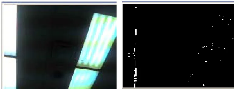
Figure 2.7: a) An image of scene has a

Variant lightening

b) The image after background

subtraction, the variation of light

2.7 Markov Chain Monte Carlo

Real use of Markov chains started during World War II [Zhu05]. Monte Carlo

method is a computational algorithm for sampling that depends on repeatedly random

sampling to find the result [Katan09]. Since it includes repeated complex calculations it is

a computer-based method. Generally, the Monte Carlo method is used for physical

simulations, mathematical problems and computer applications for different purposes

such as optimization, integration/computing and learning. A few examples of these are

finding the best ten moves for a chess game, generating random users for a

telecommunication company with different, random states and generating a random

challenger in video games.

In the late 1990’s researchers started using MCMC for very complex genetic

inference and other biological applications [Zhu05]. The basis of the Monte Carlo

approach is to sample the large system into small, random configurations. In other words,

a large, unsolvable problem can be divided into small, solvable problems. A stochastic

process has the Markov property if the conditional probability distribution of the future

states of the process depends only upon the present state.

Markov model is a stochastic model that employs the Markov property for its own

states [Katan09]. If the state of an object in the model is fully observed then the model is

a Markov Chain model [Makris04], but if it is partially observed that means that the

model is a Hidden Markov Chain Model [Staufer03]. MCMC has been used in computer

visions applications like object tracking [Osawa07, Khan05], camera network

localization [Staufer03, Makris04] and 3D reconstruction [Dellaert00]. A simple example

of MCMC sampling is that if we had a model with different states X = {x1, x2, ...xn}; each

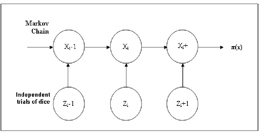
Figure2.8. MCMC generates fair samples from a probability in Ω using random numbers

(i.e. dice) drawn from uniform probability in a certain range. A Markov chain is designed

to have π(x) being its stationary (or invariant) probability [Zho05], where each state xi+1

depend upon state xi.

Figure 2.8: Markov chain model

2.8 Gaussian Mixture Model

A statistical mature method is used for data clustering in an unsupervised learning

model. Assume that entry/exit zones are already known, and consider these zones as K

classes. Each class can have observations with normal distribution and variance σ2.

Using the Gaussian method the observation is classified to the class that maximizes the

posterior probability for it [Makris04]. The observation (x) will be classified into the

learnt entry/exit zones y = {i = 1: n} where n is the number of entry/exit zones as

(2.5)

(2.6)

Where pi is the prior probability of each entry/exit zone. and are the

covariance and average for each ith entry/exit zone.

Observation (x) is classified to the ith entry/exit are where x P(y =iǀx) is the

CHAPTER III

RELATED WORK

Activity models based on trajectory observation for overlap FOVs camera

network are proposed in [Meingast07, Lee00]) where the spatio-temporal feature is used

to match trajectories of objects that are moving through the cameras FOVs. In

[Funiak06], an algorithm called SLAT, Simultaneous Location and Tracking, requiring

only minimal overlap of the cameras FOVs has been proposed. The model determines the

location of the observations using the object Gaussian densities. Many proposed

algorithms use the image correspondence for tracking the objects in the Camera network

FOVs. The method, correspondence camera network calibration, has overlapping FOVs

which requires image formation, epippolar geometry and projective transformation that

are between each pair of overlapped cameras FOVs [Meingast07].

[Mantzel04] introduced a distributed localization algorithm using the Kalman

filter framework on the extended epipolar geometry. However, the Kalman filter has

difficulties distinguishing between objects when the number of objects in the camera

FOVs is too numerous [Boyd99].

SLAM, Simultaneous Localization and Mapping, is proposed for localizing and

mapping the camera network nodes based on the movement of a robot which takes

pictures by its sensors to use for land-marking. The true locations of the landmarks are

then estimated by an Extended Kalman Filter (EKF) [Rekleitis06]. The method represents

the positions and orientations of cameras in 3D.

Many researchers in this field have focused on non-overlapping camera networks.

topological information of the camera network. They employ the entry/exit models to

correlate objects’ transition time between the related camera FOVs. [Makris04] used a

node to represent each entry/exit zone in the resulted graph, while [Kim09] used a node

to represent each pair of entry/exit zones in the graph model. The constructed model

works on multi-camera tracking and does not rely on correspondence between

trajectories. Makris et al. stated that correlation is inappropriate for multi-model

distribution. In other words, these models are not appropriate for high traffic places

where the moving objects have a substantial variation in speed.

Some researchers have worked on the supervised learning approaches. These

models require assumptions about the environment of the camera network [Marinakis05,

Lobaton09, Rahimi04]. Marinakis and Dudek proposed a Markov Chain Monte Carlo

(MCMC) model to recover the camera network topology. A Monte Carlo Expectation

Maximization is used to maximize the likelihood of the observation which minimizes the

functional usage of the Markov chain sampling. The model used environmental

assumptions as input parameters.

Rahimi et al. proposed a model that requires assumptions about the object

transiting manner. The camera position is estimated by encoding a prior learning of the

locations and velocity of targets in the Markov model. Then they calibrate this prior

learning with the camera calculations to produce posterior probability of the observations

trajectory. Even though the model works for a large number of cameras, around ten

down-facing cameras in the experiments, the result was not fully accurate since they tried

to a 3D-representation of the output model. In addition, the weakness of this approach is

Lobaton et al. used an algebraic approach simplicial representation, called the

CN-complex, which can be constructed from discrete local observations. They utilize this

representation to recover topological information of the camera network. Each camera

performs a local computation to extract the discrete observation and convert it into a

symbolic representation to reduce the cost of data communications. Then it analyzes this

symbolic representation to build a model of the environment. This approach overcomes

the restrictive input assumptions. Figure3.1 shows the simplicial representation of the

CN-Complex vectors of the overlap cameras FOVs Areas: {[1], [2], [3], [4], [5], [1 2], [2

3], [2 4], [2 5], [3 5], [4 5] and [2 4 5]}. The major drawback of this work is that each

camera has to have a processor.

Detmold et al. proposed a scalable system for automatic and online estimation of

activity topology. The model used multi-processing video streams collectively instead of

a camera unit basis processing. They used the Exclusion method that simply indicates if a

camera’s FOV is occupied, and that another camera’s FOV is unoccupied

simultaneously. Thus, the two cameras cannot be observing the same space. One major

drawback of this model is the slow processing and lack of memory usage due to the huge

number of camera nodes in the network.

Table 3.1: Approaches are used for camera network localization

Overlap Non overlap Communication Algebriac Input Unsupervised Supervised Applied Method

Meingast07 √ Feature-based

Makris04 √ √ MCMC

Lee00 √ Feature-based

Funiak06 √ SLAT

Mantzel04

Lobaton09 √ √ √ CN-Complex

Bulusu00 √ GPS

Marinakis5 √ √ √ MCMC

Mardini10 √ RSSI

Savarese02 √ √ Estimationv node

position

Rahimi04 √ √ √

Kim09 √ √ MCMC

Rekleitis06 √ √ √ SLAM

Wen10 Cloud Computing

Table 3.1: summarizes the research models in camera network localizing field in

computer vision and computer network laboratories. Some of the methods supervised the

agents transitions in scene, some others rely on an overlap camera network, while some

others have non-overlapped camera network with unsupervised learning. The rest of the

approaches used a communicated camera network and one used an algebraic approach.

Much work has been done in computer network laboratories using ultra-sound,

radio waves and GPS technology. These models utilize the communication methods

among the camera network nodes to localize the cameras positions. [Bulusu00] solves the

problem of finding locations of camera network nodes by using the triangulation (GPS)

called Received Signal Strength Indicator (RSSI) that exists in the physical layer of the

network to locate the position of a sensor in a camera network.

[Savarese02] proposes a two-phase method that depends on the connectivity of

the initial position to estimate the new network sensors’ location. All network models can

be implemented on the vision based sensor network to localize their positions, but in this

case a wireless connection is needed for the network’s nodes. Wen et al. proposed

[Wen10] a Cloud computing based algorithmic framework to for Multi-Camera Topology

Inference. The comprehensive approach uses thousands of cameras for online smart city

CHAPTER IV

DESIGN AND METHODOLOGY

We propose a Dynamic approach for recovering the topological information of a

camera network using the statistical information of the moving objects through the

networked camera FOVs. The input of our method is a set of videos of the cameras

FOVs. First, the model records the statistical information of each observation then it

learns the entry/exit zones. The model generates more observations based on the detected

observations. The generated observations are classified into learned entry/exit zones.

After that, the model detects the related cameras and calculates the transition time

between each pair of related cameras. The output of our model is a Markov model for the

networked cameras.

4.1 Observation Detection

Inference camera network topology starts reading the video that is supplied from

the networked cameras FOV. Each video is divided into frames; the frame is the image of

the scene at any particular time. Then the frames will be sent to a special buffer to be the

input for the filtering process. The buffer saves the frame as an RGB matrix, then the

filter reads the frames from the buffer and applies the Weiner filter to filter the frames of

unwanted noise. The noises have four levels which are red, green, blue and alpha level.

The default is the alpha noise level to reduce the white noise that mainly comes from the

variant lights in the corridors.

The rapid movement in-between frames get detected and the entrance of an object

is identified by comparing the rapidly changed pixels in the new series of frames to the

previous state of the settled down frames. The exit of an object is detected by noticing the

rapid change in movement to the settled down frames. We construct the blob box around

the moving object by defining the upper left corner and the lower right corner of the

moving pixels in the frame. The centroid point of the object is defined as the center of the

blob box.

Table 4.1: Sample of detected observations

Entry/Exit Row # 

Entry/Exit column # 

Event time 

Camera # 

7  20  15  c1 

29  8  49  c2 

7  20  66  c1 

28  9  103  c1 

6  19  119  c1 

7  20  168  c1 

6  17  217  c2 

29  10  245  c1 

In our system we detect the entrance and exit of each observant object (O), as a

result, whenever an object enters or exits we assign an ID to the object. Then we register

the entry/exit point (the object’s blob centriod point) in 2D (X-axis and Y-axis), as well

as the entry/exit time. Our observation detector works for live camera videos.

The problem we are facing here is the unexpected small movement in the

recording environment, such as trees’ leaves moving in the window. We overcome this

problem by using the concept of sensitivity of movement which is predefined before

detecting the motion [Lee09]. That means we threshold the speed and the quantity of

movement that will be considered as a movement. A real time organizer is provided to

register each entry/exit instant time. The time organizer makes sure that all cameras start

recordings at the same time in the network.

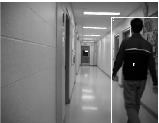
Figure 4.2: a) The moving person b) The grid of the 24 x 30 boxes

Figure 4.5 Illustrates how the moving pixels of the objects are represented in the

grid of the camera FOV. It shows the boxes that have moving objects pixels with values

4.2 Learning Entry/Exit Zones

The output entry/exit points of each camera FOV from the observation detection

phase are clustered into general classes. Then they are classified to infer the entry/exit

zones of each camera’s FOV. The method used for clustering is the Data Spectroscopy

method or DaSpec [SHI09]. We have compared this method with the general K-means

method and it has shown better results. In particular, the K-means failed to cluster two

groups of entry/exit points in their general means when they are close together. The best

example for cameras with close entry/exit zones would be when a camera FOV is looking

down a corridor that has many doors. The corridor seems to be getting narrower when the

door is further away from the camera. So the door appears small in the camera FOV and

will appear very close to the next door. Therefore, the entry/exit points detected for both

doors will be close to each other.

Figure 4.3: Detected observations entry/exit points

We have simulated a camera network with five camera FOVs and thirteen

differing, random speeds through these camera FOVs among these specified entry/exit

zones. The result from the DaSpec method was very accurate; however, this was not the

case for the K-means method. The features used for clustering are a horizontal row

number and a vertical column number of the grid’s box.

Figure 4.4: a) DaSpec Clusters b) General K-Means Clusters

Figure 4.7 Show the results of the simulation of three thousand moving agents

through five different cameras FOVs. Figure4.4 shows how the DaSpec method

succeeded to cluster the entry/exit points into thirteen groups of data which represent the

simulated entry/exit zones in the simulated network. Whereas Figure4.5 shows how the

general K-Means method could not cluster the entry/exit zones because it clusters close

groups of data that have a similar vertical or horizontal box’s numbers into same data

4.3 Computer-Generating Observations and Optimization using Monte Carlo

In this phase our model generates a number of random variables to be the input of

the Monte Carlo simulation. The Monte Carlo algorithm generates the observations to

increase the certainty of detecting the relationship between the entry/exit zones. Noise

that corrupts the Gaussian mixture model can be isolated by generating observations with

uniform distribution [Cho09]. The uniform distribution random number generator is

convenient for time accuracy purposes [WaterlooCh3].

The observations are generated based on the detected observations that have

known entry/exit zones. Let be the learned entry/exit zones from Section 3.2 where

and is the number of entry/exit zones in each camera. Let Oji be the

observations where K is the number of observations for each . The

following equation to calculate ( ) the number of iterations needed for the Monte Carlo

simulation:

(4.1)

Where:

sss

(4.2)

Table 4.2: Monte Carlo Simulation for generating observation

Monte Carlo Simulation Algorithm

Output( ) = MC(Input~,Z , ^

O _{, , )}

// the new generated observations data set ^

O

// Z the number of the generated observations

^

O _arbitrary

arbitrary

Repeat i = 1 .. N loop

Repeat j = 1 .. Z loop

Generate a new random displacement based on and

^

O_{j +}

^

O

end loop

end loop

MC simulation algorithm generates more observations for our model; based on

the variance for each pair of entry/exit zones to in crease the certiniaty of the relation

between them. The model consists the learnt entry/exit zones as the model states.

4.4 Detecting the Links Between each pair of Entry/Exit Zones

When using the fuzzy cognitive map to determine the relationship between each

pair of entry/exit zones to find if they are linked or not is related to the researcher’s

observations the variance of time difference can be used to determine how distances

change between observations of the cameras entry/exit zones. If the amount of the

difference (d) changes in small amount 0≤ Var(d) ≤1 that means the pair of the

entry/exit zones are linked. OtherwiseVar(d) ≥1 indicates that they are not linked.

Table 4.3: Algorithm for detecting the Linked Entry/Exit zones

Linked Entry/Exit Zones Detector Algorithm

Output(List) = LinkDetector(Input~, EE List,P)

// EE list is a List of each entry/exit Zone, each EEx contains it is Own Observations

// List is the list of the linked EE among cameras' FOV

//P is the probability matrix of the entry/exit zones

j i≠ loop Repeat for each pair of EE (EEi,EEj) where

if 0 < P(i,j) <= 0 then

) ( ), ( (

tance EEi O EEj O

sSis mahanoboli d ←

if 0≤Var(d) ≤1 then

//EEi and EEj are linked

List →addNode( EEi, EEj)

end if

Otherwise

//EEi and EEj are not linked

end if

The Mahalanobis distance between each pair of ( , ) where have the

observations Oi = {O1, O2...Ok} and have the observations = {O1, O2…Ok}

i

EE EE_j EEi

j

EE Oj

∑

=

−

₋

−

K

m im jm

T jm

im

O

S

O

O

O

1

₍

₎

)

(

Where S is the Covariance matrix:

₍

_,

₎

O

O

Cov

S

=

4.5 Calculating the Transition Time for the Linked Entry/Exit Zones

For each pair of linked entry/exit zones the histogram of Mahanobolis distances

(d) between their observations is calculated. Then the most popular histogram is

considered as the transition time between them. The most popular histogram of the

different distances can be found applying the peak finder function. The transition time

between each pair of entry/exit zones is used to determine if the cameras are overlapped

or not. First of all, it is simple to determine if two cameras have no linked entry/exit

zones, hence, they do not have overlapped FOVs. However, if they have linked entry/exit

zones between them they can be overlapped, or not overlapped with an unseen path

between them.

Let us assume that camera c1 have entry/exit zones A, B and they are linked.

Camera c2 has entry/exit zone C. Then the relationship between c1 and c2 can be

Table 4.4: Learning the relationship between pair of networked cameras

Learning relation between pair of cameras

Output (Relation) = determineRelation(Input~,c1,c2,EEListc1,c2)

//EEListc1,c2 is the entry/exit list between c1, c2

if EEListc1,c2 has no pair of linked entry/exit between c1 and c2 then

Relation is non-overlapped

Otherwise

if EEListc1,c2 has Linked entry/exit zones (A,B,C) where (A,B) c1, C c2 then

if absolute (transition_time (A, B) – ( transition_time(A,C) +

transition_time(C, B))) <= Threshold then

Relation is overlapped

Otherwise

Relation is related_unseen_path

End determineRelation

Figure 4.8 explains how the transition times between a pair of cameras entry/exit

zones determine the relationship between them. In a) t1=t2 + t3 that means the object can

cross an entry/exit zone of another camera FOV while it is going through a path in the

first camera. In contrast, b) the passing object moves from A to B in the same camera and

does not cross any other camera’s entry/exit zones.

4.6 The Output

A Markov Chain model is constructed from related cameras. Since we have a

countable number of cameras the future location of the object, in terms of what camera it

is in, depends on the current location of the object (what camera is seeing the object

currently). The undirected graph that represents the camera network is weighted by the

transition time between the cameras. This is the transition time between the related

entry/exit zones of each pair of networked cameras. So the vertices V = {v1, v2..vn}

represent the cameras with the edges and E = {e1, e2,…em} represent the paths between

the cameras. Where (n) and (m) are the number of networked cameras and the number of

edges between them, respectively. The overlapped cameras are linked by a black edge

while, the related non-overlapped camera are linked by a grey edge. The grey edge

represents the unseen path between two related cameras. The non-related cameras have

Figure 4.6: Markov model for networked camera topology

4.7 Conclusion

In this chapter the statistical approach of learning the camera network topology is

explained. First we described how the input videos are taken from the networked cameras

that are divided and saved in a buffer. Then we explained how a Weiner filter is used to

reduce the white noise coming from light variation in the input video. Followed by how

we located the centroid point of the object’s blob as an entry/exit point, as well as the

time of each entry/exit. We also determined that the Monte Carlo method is used to

generate more observations to increase the certainty of the learning entry/exit zones. For

classifying new entry/exit points we use a Gaussian mixture model for the purpose of

classifying the entry/exit point to the entry/exit zones which maximize the likelihood of

the zone. Links among cameras’ FOVs entry/exit zones are then detected from this prior

knowledge. We find the transition time by calculating between each pair of linked

entry/exit zones and the adjacency matrix of the linked entry/exit zones of the networked

cameras is analyzed to construct the output model of the relationships between each pair

CHAPTER V

EXPERIMENTAL RESULTS

We have implemented the camera network topology inference system in Borland

C++ and Matlab 7.2. We have also used VisionLab [VisionLab] tool to implement the

observation detection. We have evaluated our application with two different networked

camera locations using real videos.

5.1 Four Networked Camera

We setup a four-camera network on one floor which has crossed corridors with

different entry/exit zones. Figure 5.1 shows the camera network setup. The camera

network has some overlapped camera FOVs and some cameras that have non-overlapped

camera FOVs. For example, camera 1 and camera 2 are overlapped while camera 1 and

camera 3 are not.

Figure 5.1 shows how we locate the cameras in the environment. The pair of

camera FOVs, camera1 and camera 2, are overlapped, camera3 and camera4 are also

overlapped.

a) Camera 1 FOV b) Camera 2 FOV

c) Camera 3 FOV d) Camera 4 FOV

Figure 5.2: Experiment 1 camera FOVs

Figure 5.2 shows the networked cameras FOVs. The cameras are used are of

different manufacture, camera1 and camera 2 are Sony 10.1 mega pixel, while the other

The object detector reads the video and analyzes the entry/exit location as well as

the time of the moving objects. The output of this step is a text file with all observations.

Then we cluster the entry/exit points for each camera to find the number of classes to

infer the entry/exit zones for these cameras. The scale used for the entry/exit points is (30

x 24), which means we divided the screen into thirty rows and twenty-four columns to

simplify the computation and increase the speed of processing. We have used the Data

Spectroscopy function for this task. The top eigenvector of X-row and Y-row for each

observation are not classified until the last unsigned eigenvector value does not change.

Table5.1: Classified observations for camera 1

X-row Y-column

Class or (Entry/Exit) zone number

X-row sign eigen vector picked Y-row sign eigen vector picked 0 11 0 11 0 11 0 11 1 11 0 11 0 1 11 12 13 16 14 7 13 7 12 17 13 18 13 16 17 13 2 1 2 1 2 1 2 1 2 1 2 1 2 2 1 0.0004 0.3047 0.0117 0.2955 0.0042 0.3047 0.0042 0.2955 0.0147 0.3047 0.0095 0.3047 0.0117 0.0147 0.3047 0.0129 0.0093 0.4029 0.0070 0.0697 0.0093 0.0697 0.0106 0.4090 0.0093 0.4001 0.0093 0.0106 0.4090 0.0093

Table 5.1: shows the classified observations of camera 1. The observations were

When all camera FOVs observations are clustered and classified into the detected

entry/exit zones the Monte Carlo method generates new observations in order to

accurately detect the relationship between each pair of entry/exit zones.

a) camera 1 observations b) camera 2 observations

c) camera 3 observations d) camera 4 observations

Figure 5.3: All cameras observations are clustered into main entry/exit zones

We generated eighty-nine observations from eleven observations for each pair of

entry/exit zone 1 in camera 1 to entry/exit zone 2 in the same camera; the standard

deviation = 0.5828 and the number of iterations N = 348. After generating the new

observations the transit time was found by the peak finder to equal 7.8102, for the time

histogram, see Figure 5.4.

Figure 5.4: Histogram of the transit time of the observations

Figure 5.4: represents the histogram of the transit time of the observations that

were generated by Monte Carlo method based on the observations detected between

entry/exit zone 1 and entry/exit zone 2 in camera 1. The most popular histogram equals

7.8102.

After finding the transition times by the Monte Carlo method between each pair

of the learned entry/exit zones then an adjacency matrix is constructed based on the

related entry/exit zones and transition time. If the variance of the Mahalanobis distances

is lower than one then they are related. Since the objects are moving in a consistent way

around the cameras all the entry/exit zones are related in this experiment. Therefore, the

variance of the Mahalanobis distance between pairs of entry/exit zones is smaller than

one for all pairs of entry/exit zones. The transition time is computed by finding the most

popular histogram of the different distances between the pairs of entry/exit zones.

Table 5.2: The adjacency matrix of transition time

E/E# 1 2 3 4 5 6 7 8

1 0 7.8102 12.35 0.95 19.95 17.1 25.65 21.85

2 7.8102 0 2.3 8.25 29.45 9.1 0 0

3 12.35 2.3 0 10.5 1.65 26.6 0 0

4 0.95 8.25 10.5 0 11.55 16.15 14.85 20.9

5 19.95 29.45 1.65 11.55 0 5.1 3.9 0.991

6 17.1 26.6 26.6 16.15 5.1 0 0.55 3.95

7 25.65 0 0 14.85 3.9 0.55 0 4.9167

8 21.85 0 0 20.9 0.991 3.95 4.9167 0

Table 5.2: The adjacency matrix is constructed depending on the relation between

each pair of entry/exit zones among the networked cameras. The networked cameras have

eight entry/exit zones among them.

The relationship linking cameras are determined by the transition times between

the entry/exit zones among cameras. We used a threshold of T =0.200 seconds for

detecting the cameras overlapping See 5.4.

Table 5.3: Detecting the overlapped cameras FOVs in the camera network

Cam1 Cam2 Cam1 EE#A Cam1 EE#B Cam2 EE#C Transition time C-A Transition time C-B Transition time A-B

2 1 3 4 2 2.3 8.25 10.5

3 4 5 6 8 0.991 3.95 5.1

Table 5.3: shows the results of the detected pairs of overlapped camera FOVs. For

example, camera 2 is overlapped with camera 1, camera 1 has entry/exit zone 2 and

camera 2 has related entry/exit zones 3 and 4. The summation of the transition time from

entry/exit zone 2 to entry/exit zone 3 and the transition time from entry/exit zone 2 to

entry/exit zone 4 is approximately equal to the transition time from entry/exit zone 3 to

entry/exit zone 4.

The Markov model shows the overlapped camera FOVs is shown in Figure 5.6

Figure 5.5: The camera network topology

5.2 Five Networked Camera

We set five networked cameras on the same floor of a building which has crossed

corridors with different entry/exit zones. Figure 5.6 shows the camera network setup. The

camera network has some overlapped cameras FOVs and some cameras have

cameras while camera 3 is overlapped with camera 4, camera 5 and non-overlapped with

camera1 and camera 2.

Figure 5.6: Experiment 2 setup

Figure 5.6 shows how we locate the cameras in the environment. The pair of

camera FOVs, camera1 and camera 2, are overlapped, camera3 and camera4 are also

a) Camera1 FOV b) Camera 2 FOV

c) Camera 3 FOV d) Camera 4 FOV

e) Camera 5 FOV

Table5.4: Overlapped Camera FOVs in experiment 2

Cam1 Cam2 Cam1 EE#A Cam1 EE#B Cam2 EE#C Transition time C-A Transition time C-B Transition time A-B

1 2 1 2 3 9.9 2.85 13

2 1 3 4 1 10.2 3 13

2 1 3 4 2 2.85 10.5 13

2 5 3 4 10 11.75 1.05 13

2 5 3 4 11 9.75 3.05 13

3 4 6 7 9 1.6 3.3 4.45

5 1 10 11 1 2 0.35 2

5 3 12 13 6 3.55 1.15 4.7

5 4 12 13 9 3.7 7.55 10.65

Table 5.4 shows the result of detecting the overlapped cameras FOVs. For

Experiment 2 the threshold is used for this example is T = 0.450; when we used 0.250 we

missed one link between camera 4 and camera 5.

The Markov model shows the overlapped camera FOVs is shown in Figure 5.8

CHAPTER VI

CONCLUSIONS AND RECOMMENDATIONS

6.1 Conclusion

In this thesis we have proposed a MCMC model to recover the topological

information of a camera network depending on the statistical information of the moving

objects in the cameras’ FOVs. The networked cameras’ FOVs can be overlapped or

non-overlapped, and communication between the network nodes is not necessary. The

unsupervised learning model requires no assumption on the input parameter to construct

the topology of the camera network. Many applications in the smart video surveillance

field can benefit from this work.

We have analyzed the videos from the networked cameras to determine the

needed information to infer the camera network topology. We have used an observation

detector to detect the entry/exit points and time by detecting the centroid points of the

objects’ blobs. The model learnt the entry/exit zones of each camera FOV using the Data

Spectroscopy algorithm. Then we generate more observations using the Monte Carlo

method and we classify the new observations into learned entry/exit zones.

The proposed model uses a Fuzzy cognitive decision to determine the relations

between the cameras entry/exit zones. The variance of the Mahalanobis distances

between the closest pairs of observations time of the entry/exit zones is used to decide

whether the entry/exit zones are related or not. The results of the entry/exit zones are

saved in an adjacency matrix. The next step is to find the overlapped cameras FOVs

chain graph of the related cameras. The relative location of each camera to the others is

shown in a graph representation.

6.2 Future Work

Although the object detector has been already implemented for this work we are

aiming at implementing a real life system of this problem. In this case, big network

hardware is needed to be set for a real life application, such as processors for each node

as well as a wireless communication among of them.

A variant of traffic types experiment needs to be tested for this approach, such as

a high speed traffic road and a building with multi-floor setting camera network or, a

senior citizen care centre experiment. The smart care centre application can benefit from

this work. For low traffic experiments, the application needs to run for a longer time and

it might need supervised agents to be moving in the cameras’ FOVs. For example, a fire

exit door in a building might not be used in the experiment time, but in reality, it is used

in emergencies. In this case, a supervised agent or a person can be guided in using these

doors

The threshold of the camera overlap detector needs to be overcome or at least it

can be minimized further. For this purpose, choosing the observation process can be

enhanced by adding a criterion to select the convenient observation for a specific kind of

REFERENCES

[Akyildiz07] Akyildiz, I.; Melodia, T.; and Chowdhury, K.; “A survey on wireless

multimedia sensor networks”, The International Journal of Computer

and Telecommunications Networking, 51(4), p.921-960, March 2007

[Ali06] Ali, M. A.; "Feature-Based Tracking of Multiple People for Intelligent

Video Surveillance", Master's Thesis, School of Computer Science,

University of Windsor, 2006

[Andrieu03] Andrieu, C.; Freitas, N. D.; Doucet, A.; Jordan, M. I.; “An

Introduction to MCMC for Machine Learning, Machine Learning”,

Volume 50, pp 5–43, February 2003

[Boyd99] Boyd, J. E.; Meloche, J.; and Vardi, Y.;"Statistical tracking in video

traffic surveillance", The Proceedings of the Seventh IEEE

International Conference on Computer Vision, Volume.1, pp.163-168,

September 1999

[Chavel78] Chavel, P.; and Lowenthal, S.; "Noise and coherence in optical image

processing. II. Noise fluctuations", Optical Society of America,

Volume 68, pp. 721–732,August 1978

[Chilgunde04] Chilgunde, A.; Kumar, P.; Ranganath, S.; WeiMin, H.;

”Multi-Camera Target Tracking in Blind Regions of ”Multi-Cameras with

Non-overlapping Fields of View”, The Proceedings of The British Machine

Vision Conference BMVC, September 2004

[Cho09] Cho, E.; Downes, I.; Wicke, M.; Kusy, B.; Guibas, L. J.;” Recovering

Conference on Embedded Networked Sensor Systems, 387-388,

Novermber 2009

[Clarot09] Clarot, P.; Ermis, E.; Jodoin, P.; Saligrama, V.; "Unsupervised camera

network structure estimation based on activity", Third ACM/IEEE

International Conference on Distributed Smart Cameras, pp.1-8,

August 2009

[Dellaert00] Dellaert, F.; Seitz, S.; Thorpe, C.; Thrun, S.;"Structure from motion

without correspondence", Proceedings. IEEE Conference on

Computer Vision and Pattern Recognition, Volume 2, pp.557-564,

June 2000

[Delp82] Delp, E.; Mudge, T; Siegel, L.; Siegel, H. J.;"Parallel Processing for

Computer Vision", Proceedings of the SPIE Conference on Robot

Vision, Volume 336, pp. 161-167, May 1982

[Durand00] Durand, F.; “A multidisciplinary survey of visibility”, in: ACM

SIGGRAPH course notes, Visibility, Problems, Techniques, and

Applications, July 2000

[Funiak06] Funiak, S.; Guestrin, C.; Paskin, M.; Sukthankar, R.; "Distributed

localization of networked cameras", The Fifth International

Conference on Information Processing in Sensor Networks, pp. 34-42,

2006.

[IEEE-CV] http://ieeexplore.ieee.org/xpl/conhome.jsp?punumber=1000149,

November 12th, 2010

and multiple target tracking usingmobilerobots”, Master’s Thesis,

Rensselaer Polytechnic Institute, December 2007

[Kandasamy07] Kandasamy, W.; Smarandache, F.; and Ilanthenral, K.; “Elementary

Fuzzy Matrix Theory and Fuzzy Models for Social Scientists”,

Technical Report, 2007

[Katan09] Kattan, M. W.; Cowen, M. E.; "Encyclopedia of medical decision

making", SAGE. Publications ,Inc. , Volume 2, Decision Trees, pp.

345-346, 2009

[Khan05] Khan, Z.; Balch, T.; and Dellaert, F.; "MCMC-based particle filtering

for tracking a variable number of interacting targets", IEEE

Transactions on Pattern Analysis and Machine Intelligence, 27(11),

pp.1805-1819, November 2005

[Kim09] Kim; H.; Romberg, J.; and Wolf, W.;"Multi-camera tracking on a

graph using Markov chain Monte Carlo", ICDSC 2009. Third

ACM/IEEE International Conference on Distributed Smart Cameras,

pp.1-8, September 2009

[Ksantini09] Ksantini, R.; Shariat, F.; and Boufama, B.; "An Efficient and Fast

Active Contour Model for Salient Object Detection", 2009 Canadian

Conference on Computer and Robot Vision CRV, pp.124-131, May

2009

[Learn-NT]

http://learn-networking.com/network-design/a-guide-to-network-topology, December 17th, 2010