Modified VM-Assign Load Balancing Algorithm of Cloud Computing in CloudSim

(1)

Modified VM-Assign Load Balancing

Algorithm of Cloud Computing in CloudSim

Prithpal Mohini Singh 1, Shaveta Angurala 2

P.G. Student, Department of Computer Science, DAV Institute of Engineering and Technology, Jalandhar, India 1

Assistant Professor, Department of Computer Science, DAV Institute of Engineering and Technology, Jalandhar, India2

ABSTRACT: In Cloud Computing one of the major challenges is efficient and effective utilization of resources to obtain quick response time and improve the performance of the Cloud Configuration. Different Load Balancing Techniques are developed for proper scheduling of available resources to effectively the overutilization or underutilization of resources. The paper presents and implements available load balancing algorithms with the proposed Modified Load Balancing Algorithm to improve the performance of the Cloud. CloudSim is implemented and results of the Load Balancing Algorithms are compared using parameters like Response Time and Data Processing Time The paper aims to provide the proposed Modified Load Balancing Algorithm a combination of three different methods, Batch Processing, Defined Value and Priority Algorithm, to balance the scheduling of load and for proper utilization of resources in Cloud Computing environment. The paper also provides comparative analysis of the proposed Modified Load Balancer with the existing Optimal Load Balancer Algorithm to analyse the results using Cloud-Analyst simulator using parameters like Response Time and Data Processing Time to get optimized results. It considers and implements four different case studies for comparing these parameters of the Load Balancing Algorithm to properly schedule available resources for better performance. The results showed optimized results on response time and Data Processing Time improving the performance and efficiency of the Cloud.

KEYWORDS: Cloud Computing, Scheduling, Load Balancing, Virtual Machines, Response Time, Utilization, Virtualization, Modified Load-Balancer, Data Processing Time, Cloud-Analyst, Simulation.

I. INTRODUCTION

The Cloud computing is defined as a model for enabling convenient, on-demand network access to a shared pool of configurable computing resource which includes networks, servers, storage, applications and services that can be rapidly provisioned and released with minimal management effort or service provider interaction. Cloud Computing, service model is defined as different types of applications provided by different servers across the cloud which is categorised as three types of service models, i) Software as a Service (SaaS), ii) Platform as a Service (PaaS), ii) Infrastructure as a Service (IaaS) and, private, public, hybrid and community are the four deployment models of Cloud Computing[1].

The process of distributing the total -load to the individual nodes/datacenters of the collective system to improve both resource utilization and job response time where resources are neither over-utilized or under-utilized , is called Load Balancing[2]. The main motive of load balancing is to achieve optimal resource utilization, Uniform distribution of load at different data centers, improving the overall performance of the system, higher user satisfaction, faster Response, and system stability[3][4]. The Load Balancing Algorithms are of two types, static and dynamic load balancing algorithms[5].

(2)

This parameter should be minimized for the better performance of the cloud. Second metric focuses on minimum, average and maximum time taken to process a task. This metric should be minimized for better efficiency of the system.

II. RELATED WORK

In [7] this paper, the authors proposed optimal-load balancing algorithm to check the overutilization or underutilization of resources or requests on cloud which are controlled and handled by VM to process the requests for better performance, throughput, response time. In [8] this paper, an algorithm for load balancing in cloud computing is

implemented foraging the behavior of honey bees . When overloaded virtual machine is found, then the task is to be

(3)

III.PROPOSED ALGORITHM

A. Design Considerations:

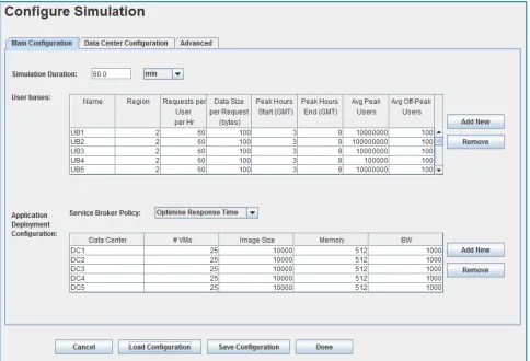
 For Main Configurations, the Simulation time is 60 mins.

 User-Bases up to 5 are set for different geographical locations, Request Per-User-Per Hour value is set up to 60, and Data-Size-Per Request (in bytes) is 100.

 Application Service Center describes two parameters as Service Broker Policy: Response Time, Data Processing Time.

 For Data Centers, Case Studies from VM to 75 are considered; image size 10000, memory 512 and BW 1000 are set as default values.

 Figure 1 shows the GUI used to configure the specifications for User-bases, and Application Deployment Configuration, where the Data centers, Virtual Machines and other entities can be specified and defined as per simulation requirements.

Figure 1 Configure Simulation of Cloud Analyst Simulator

B. Description of the Proposed Algorithm:

(4)

data processing time with the Optimal Load Balancing Algorithm hence reducing the cost and maximizing the performance of the Cloud Environment. The Proposed Algorithm Modified-VM Load Balancer Algorithm combines batch processing, Priority Algorithm and Defined Value to get faster response time, lower data processing time, reduced cost and efficient performance. It overcomes the flaw of not assigning the next/ incoming user-request to the VM which was allocated in the previous assignment as batch is used to allocate requests which saves time of comparison of individual VMs apart from checking for their availability, current allocation time and whether it was used in the previous request or not. In this case the response time of the algorithm could degrade and hence reduce the performance of the Cloud. The Modified Load Balancer firstly checks for the number of user-requests to be served and allocated though a function called Batch, which specifies the batch size and the maximum capacity of load allocation on individual VMs/Resources based on number of jobs/user-requests received. The Algorithm then calculates the current allocation of individual VMs and selects the maximum value of current allocation count. The defined value is calculated for every VM by deducting the Current allocation size from the maximum capacity that can be allocated to every VM (maximum capacity of individual VMs is decided by the batch function depending on the number of user-requests received). The defined value is then compared with the Maximum current allocation value for every VM, to set priority on individual VMs. The highest defined value means lesser user-requests are allocated to the VM; hence higher priority, so the higher defined values get high priorities to which batch of user-requests/jobs can be allocated. After allocating the VM, it updates the allocation table and calculates the defined values again for comparison and prioritizes the VMs for task/job allocation. Instead of parsing the table, checking the availability status, and the last assigned VM every for single user-request as specified in Optimal Scheduling. The proposed Algorithm parses Allocation table for batch of user-requests, thereby reducing the number of comparisons and certain conditions which leads to faster response time and better performance of the system.

Step 1: Calculating the Data Load:

Suppose there are ‘n’ numbers of user-base requests in different regions that need to be scheduled

R= { , , , , … . . , } (1)

If there are ‘m’ set of Virtual Machines at every Data Center or Region

V= { , , , , … . . , } (2)

The Data Load can be defined by L = {V} * {R}

= { , , , , … . . , } (3)

A method/function f(R) needs to be defined so as to map the set of request or load can be distributed to Virtual

Machines available at different geographical locations to get optimized result for balancing load by considering

≈ ≈ ,≈ ≈ . . , ≈ } (4)

Let us use σ to reflect the time needed for executing task Lo on the Virtual Machine Vi, time required to process all

requests/tasks at will be = ∑ _∈ ₍ ₍ ₎₎ (5)

The numbers of Virtual Machines are given by ‘m’. When m = 1, only one Virtual Machine is used to execute the

user-based requests or tasks. The time taken to complete serve all the requests on given machine is the sum total of the tasks

that are executed by the virtual machine: T = ∑ (o = 1 to n ) (6)

For Multiple virtual Machines, m>1, the user requests can be shared and executed by different virtual machines

depending on the availability of the server in different regions.

(5)

Step 2 Selection Criteria:

The Proposed Technique to balance load in the Cloud by scheduling requests/jobs to get optimized response time as compared to the previous Optimal Load Balancing Technique, implements three techniques to get better results and faster response time than the base algorithm. The Proposed Method implements Batch Processing, Defined Value and Priority Scheduling to allocate the VMs to the user requests or tasks. The Batch Processing works based on the number of user-requests received. If the number of user-requests are less than or equal to 100, then the batch size to be allocated to the VM is 5 and the maximum capacity of the load that can be allotted to the VMs is 90. To generalize the batch processing function formulae:

Batch (If UserReqN <= 100, then Batch_size = 5 AND MaxAllocCapacity = 90. ……… If UserReqN <= N, then Batch_size = .05N AND MaxAllocCapacity = .9N)

Step 3: Assigning the Load to VMs at different Geographical Locations.

For Every VM calculate the Defined Value as, Defined_Value = MaxAllocCapacity – CurrAllocVal. The Modified Load Balancer selects the MaxCurrAllocValue for comparison with the Defined Values.

Assigns Priority to every VM based on Defined value, highest_priority to the Highest (Defined_Value), so on and the lowest_priority to the least Defined_Value. The Load Balancer then selects the VM and allocates Batch to it.

IV. PSEUDO CODE

Input: No of incoming user-requests R1, R2 . . . .. Rn.

Available The number of VMs; VM1, VM2 . . . VMn.

Output: All incoming user-requests R1, R2 . . . ... Rn are allocated according to the batch function and

priority is assigned according to DefVal of individual resources among the available VMs; VM1, VM2 . . . VMn.

Step 1: Initially all the VM's have 0 allocations. Initialize VMs = 0;

Step 2: Modified VM-assign load balancer maintains the Allocation table of VMs which has no. of requests currently allocated to each VM, DefinedValue, Priority of VMs.

VM(id, State, CurrentAllocationValue, DefinedValue, Priority);

Step 3: When user requests arrive at the data-center, it passes the jobs over to the load balancer.

Step 4: The function Batch is defined,

Batch (UserRequestN, NB, MaxAllocCapacity)

(If (UserRequestN <= 100) then NB = 5 AND MaxAllocCapacity = 90. If (UserRequestN <=10000) then NB = 500 AND MaxAllocCapacity = 9000. ... ………

If (UserRequestN<=n) then NB = .05n AND MaxAllocCapacity = .9n;) Step 5: Calculate the CurrentAllocationValue on every VM.

Step 6: For every VM/Resource Defined Value is calculated by subtracting the Current Allocation value of user requests from the Maximum Allocation value, which specifies the maximum load/maximum number of user request that can be allocated to a VM and is specified by the batch function DefValue = MaxAllocVal – CurrentAllocationValue.

a. For Every VM, Compare the DefinedValue with the Max(CurrentAllocationValue) and Check and parse table for the condition and value to assign priority to every VM; For (Max(DefinedValue)= priority; priority++):

Select Max(DefinedValue); assign VM( priority). Cases:

(6)

Return to Step a.

b. Allocate the batch() to the VM( highest _priority). Update VM(CurrentAllocationValue).

Return to Step 5.

Step 7: A Response is received at the Data-Center after VM has finished the user-request/job. Step 8: The data center notifies the Modified VM-assign load balancer for the VM de-allocation and updates the table;

Step 9: Return to Step 2.

V. SIMULATION RESULTS

The simulation studies involve Case Studies of VMs from 5 to 75 at each Data processing Center located at different Geographical locations. The proposed Modified Load Balancing algorithm is implemented with CloudSim( CloudAnalyst). Proposed algorithm is compared by two parameters Response Time and Data Processing Time. Response Time is the amount of time that is taken by a particular load balancing algorithm to response a task in a system. This parameter should be minimized for better performance of a system. Data Processing Time is the amount of time actually needed to process a task. The performance of the Load Balancing algorithms is measured by considering the parameters like response time and data processing time.

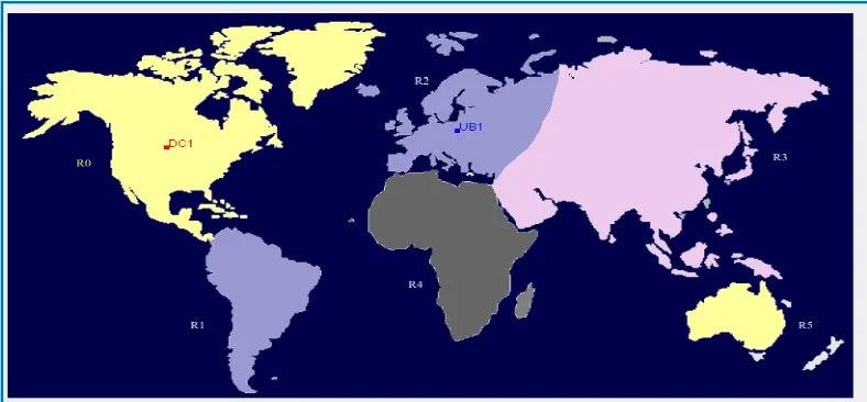
Figure 2 displays Cloud-Analyst Simulator which shows Data Centres, Regions, and User-Base at different geographical Locations. Table 1 shows the Comparative Response time (ms) for the Load Balancing Algorithms when different case scenarios are used to study the impact of increasing the number of VMs at different data centres. Table 2 shows the Comparative data processing time (ms) for the Load Balancing Algorithms for different case studies. Table 3 displays the Comparative average response time of the load balancing algorithms. Figure 3 shows graphical comparison of the algorithms for parameters average response time and average data processing time. Table 4 shows the percentage improvement/ optimization in average response time for the load balancing algorithms. Table 5 show the results of different case studies of VM from 5 up to 75 for average data processing time then calculates the difference in the data processing time for the two algorithms.

Figure 2 Cloud Analyst Simulator: Region.

(7)

better is the performance and of the efficiency of the algorithm. For every case study, the proposed algorithm shows faster response time.

Table 1Comparison Table for Response Time (ms)for Different Case Studies

CASE STUDY ALGORITHM Avg(ms) Min (ms) Max (ms)

CASE 1: VMs=5

Optimal Load 385.34 37.61 18053.02

Modified VM-Load Balancer 262.14 37.61 16398.55

CASE 2: VMs=25

Optimal Load 1137.26 65.25 36691.79

CASE 3: VMs=50

Optimal Load 387.84 37.62 17752.26

CASE 4: VMs=75

Optimal Load 355.35 36.86 18053.50

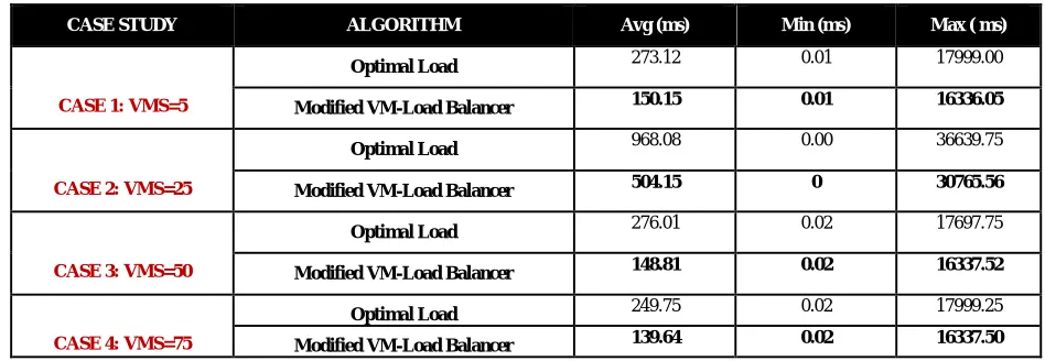
Data Processing timeis the amount of time actually needed to process a task. Considering the same case studies form VM 5 to 75, for optimizing the data processing time of the existing Optimal Load Balancer and comparing and analysis results with the Proposed Modified Load Balancer Technique. The results clearly display optimized results where average, minimum and maximum time(in ms) for data processing time are better than the previous algorithm, Optimal Load balancing algorithm.

Table 2 Comparison Table for Data Processing Time for Different Case Studies

CASE STUDY ALGORITHM Avg (ms) Min (ms) Max ( ms)

CASE 1: VMS=5

Optimal Load 273.12 0.01 17999.00 Modified VM-Load Balancer 150.15 0.01 16336.05

CASE 2: VMS=25

Optimal Load 968.08 0.00 36639.75 Modified VM-Load Balancer 504.15 0 30765.56

CASE 3: VMS=50

CASE 4: VMS=75

(8)

Table 3 Load Balancing Algorithms Comparison

ALGORITHM AVG RESPONSE TIME (ms) AVG DATA PROCESSING TIME (ms)

OPTIMAL LOAD 2264 1766

MODIFIED LOAD 1439 941

Figure 3 displays the results that are obtained from table 3 where average response time and average data processing time are compared and difference in the optimized results are displayed and compared using graphs for algorithms.

Figure 3.Comparison Optimal Load Balancing Algorithm and Modified Load Balancing Algorithm

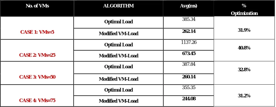
Table 4 displays the improvement in average response time when the proposed and existing algorithms are compared for the case studies from VM 5 to 75. In every case, Modified VM-Load algorithm displays faster response time. The difference in the change shows the optimized percentage of the algorithms.

Table 4 Percentage Improvement/Optimization in Response Time

No. of VMs ALGORITHM Avg(ms) %

Optimization

CASE 1: VMs=5

Optimal Load 385.34

31.9%

Modified VM-Load 262.14

CASE 2: VMs=25

40.8%

CASE 3: VMs=50

32.8%

CASE 4: VMs=75

31.2% Modified VM-Load 244.08

0 500 1000 1500 2000 2500

Optimal Load Balancing Modified Load Balancing

(9)

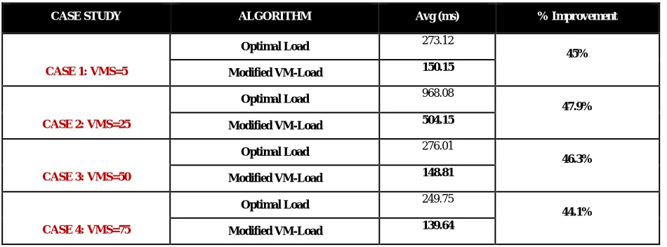
Table 5 displays case studies from VM 5 to 75 and compares the average Data processing time for the two algorithms to exhibit which algorithm faster processing and the percentage optimization shows by how much the time improved and hence the efficiency of the cloud. The Optimal Load shows more data processing time in every case and the proposed algorithm shows faster and better average data processing time and the percentage improvement in overall time.

Table 5 Percentage Comparison in Data Processing Time for different Case Studies

CASE STUDY ALGORITHM Avg (ms) % Improvement

CASE 1: VMS=5

45%

CASE 2: VMS=25

47.9%

CASE 3: VMS=50

46.3%

CASE 4: VMS=75

44.1%

VI.CONCLUSION AND FUTURE WORK

The simulation results showed that the proposed algorithm, Modified Load Balancing Algorithm performs better than the Optimal Load balancing Algorithm with parameters like Response time and Data Processing time displaying optimized results and better performance. Each case study takes different values of VM to study the impact of algorithm by increasing load and resources at different geographical regions. The impact of the proposed algorithm can be further studied by increasing the number of user requests or tasks to be performed. Further case studies can be conducted by increasing the user requests and number of VM allotted at different data centers (scaling up the configuration of the cloud environment), using parameters like response time and data processing time for the load balancing algorithms. The performance of the proposed algorithm Modified VM-assign Load Balancing Algorithm is analyzed by two parameters, in future with some modifications in pseudo algorithm, and more parameters like fault tolerance, CPU utilization, resource utilizations can be considered to check and upgrade the performance of the proposed algorithm and can be further compared with other load balancing algorithms. Optimized Load Balancing helps in proper utilization of resources so they are neither over-utilized nor underutilized thereby minimizing resource consumption.

REFERENCES

1.“NIST Cloud Computing Program–NCCP”,Nov 2010. [Online]. Available:https://www.nist.gov/programs-projects/nist-cloud-computing-program-nccp.

2. V.Suresh Kumar, “Resource Scheduling for Load Balancing Using Ant Colony Optimisation”, Vol 117, No. 22, 2017. 3. Foram F. Kherani, and Prof. Jignesh Vania, “Load Balancing in Cloud Computing", IJEDR, Vol 2, Issue 1, 2014.

4. D. Chitra Devi, and V.Rhymend Uthariaraj, “Load Balancing in Cloud Computing Environment Using Improved Weighted Round Robin Algorithm for Nonprememtive Tasks, Scientific World Journal, Vol 2016.

(10)

7. Shridhar. G. Donamal, "Optimal Load-Balancing in Cloud Computing by efficient utilization of virtual resources", IEEE, 2014 Sixth International Conference on Communication Systems and Networks (COMSNETS), Jan 2014.

8. Obaid Bin Hassan et al, “Optimal Load Balancing of Cloudlets using Honey Bee Behaviour Load Balancing Algorithm”, International Journal of Advance Research in Computer Science and Management Studies, Vol 3, Issue 3, 2015.

9. Saeed Javanmardi, MohammadShojafar, Danilo Amendola, and Nicola Cordeschi, “ Hybrid Job scheduling Algorithm for Cloud computing Environment”, Proceedings of the Fifth International Conference on Innovations in Bio-Inspired Computing and Applications IBICA 2014, Vol 3, pp 43-52, 2014.

10. Gulshan Soni and Mala Kalra,” A Novel Approach For Load Balancing In Cloud Data Center”, 2014 IEEE international advance computing conference (IACC), pp 807-812, 2014.

11. Hitesh A. Ravani, Hitesh A. Bheda, and Vruda J Patel, “Genetic Algorithm Based Resource Scheduling Technique in Cloud Computing”, International Journal of Advance Research of Computer Science and management Studies, Volume 1, Issue 7, 2013.

12. Dhinesh Babu L.D., and P. Venkata Krishna, “Honey Bee Behavior Inspired Load Balancing Of Tasks In Cloud Computing Environments”, Applied Soft Computing Journal, Vol. 13, Issue 5, pp 2292-2303, 2013.