Application of an Optimized Expert System in Development of Simplified Turbomachinery Modelling

University of Windsor University of Windsor

Scholarship at UWindsor

Scholarship at UWindsor

Electronic Theses and Dissertations Theses, Dissertations, and Major Papers

2017

Application of an Optimized Expert System in Development of

Application of an Optimized Expert System in Development of

Simplified Turbomachinery Modelling

Simplified Turbomachinery Modelling

Matheson West University of Windsor

Follow this and additional works at: https://scholar.uwindsor.ca/etd

Recommended Citation Recommended Citation

West, Matheson, "Application of an Optimized Expert System in Development of Simplified Turbomachinery Modelling" (2017). Electronic Theses and Dissertations. 7406.

https://scholar.uwindsor.ca/etd/7406

This online database contains the full-text of PhD dissertations and Masters’ theses of University of Windsor students from 1954 forward. These documents are made available for personal study and research purposes only, in accordance with the Canadian Copyright Act and the Creative Commons license—CC BY-NC-ND (Attribution, Non-Commercial, No Derivative Works). Under this license, works must always be attributed to the copyright holder (original author), cannot be used for any commercial purposes, and may not be altered. Any other use would require the permission of the copyright holder. Students may inquire about withdrawing their dissertation and/or thesis from this database. For additional inquiries, please contact the repository administrator via email

Application of an Optimized Expert System in

Development of Simplied Turbomachinery

Modelling

by

Matheson West

A Thesis

Submitted to the Faculty of Graduate Studies

through the Department of Mechanical, Automotive & Materials Engineering in Partial Fulllment of the Requirements for

the Degree of Master of Applied Science at the University of Windsor

Windsor, Ontario, Canada 2017

Application of an Optimized Expert System in

Development of Simplied Turbomachinery

Modelling

by

Matheson West

APPROVED BY:

N. Biswas

Department of Civil & Environmental Engineering

B. Minaker

Department of Mechanical, Automotive & Materials Engineering

J. Defoe, Advisor

Department of Mechanical, Automotive & Materials Engineering

Declaration of Originality

I hereby certify that I am the sole author of this thesis and that no part of this thesis has been published or submitted for publication.

I certify that, to the best of my knowledge, my thesis does not infringe upon anyone's copyright nor violate any proprietary rights and that any ideas, techniques, quotations, or any other material from the work of other people included in my thesis, published or otherwise, are fully acknowledged in accordance with the standard referencing practices. Furthermore, to the extent that I have included copyrighted material that surpasses the bounds of fair dealing within the meaning of the Canada Copyright Act, I certify that I have obtained a written permission from the copyright owner(s) to include such material(s) in my thesis and have included copies of such copyright clearances to my appendix.

Abstract

Simulating the ingestion of non-uniform inow to a fan or compressor requires enor-mous computational resources if the full details of the ow in the blade rows being studied is to be resolved, since full-wheel unsteady computations are required. A simplied modelling approach exists as an alternative computational option, which is the use of volumetric source terms (body forces) in place of the physical blades. Typically, body force models are manually calibrated with reference to single passage simulation results, and demands signicant user experience and expertise. The objec-tive of this thesis is to eliminate the need for experience and expertise during model calibration as much as is practical by employing an automated expert system. The modelling approach employed in this work is the combination of an existing turning force model, and an adaptation of an existing viscous force model. The automated system is implemented into Matlab and makes use of Ansys CFX as the ow solver. User input is required to initialize the system but the procedure then runs through to convergence of the nal, calibrated model. Viscous force model coecients that are traditionally found through an iterative procedure, are instead subjected to a Nelder-Mead optimization process. The machine studied as an example of the appli-cation of the automated technique is the NASA stage 67 transonic compressor. At peak eciency, the isentropic rotor and stage eciency, and the rotor work coecient are matched within 1% of their single passage counterparts, a result that is on par

Acknowledgements

The work presented in this thesis is the result of the combined eort and support of the people I am fortunate enough to have close to me. Most importantly, I am thankful for the guidance and support of my advisor, Dr. Je Defoe. I owe a great deal of the knowledge and skills I employ today to him, as he has patiently guided me over the last few years. The dedication and focus he invests into each of his students is a testament to the type of professional he is, something I am truly grateful for. Also, I would like to thank my committee members Dr. Nihar Biswas and Dr. Bruce Minaker for their time in reviewing my thesis and insightful suggestions on improvements.

To the members of the Computational Fluid Dynamics Laboratory and Turboma-chinery and Unsteady Flows groups who I was fortunate enough to cross paths with during my tenure, I would like to thank you for the advice and support you provided me that aided me in completing this thesis. Specically, I would like to acknowledge David Jarrod Hill, Kharuna Ramrukheea, Quentin Minaker, and Kohei Fukuda.

As well, I would like to acknowledge the nancial support I was granted from the Natural Sciences and Engineering Research Council.

Contents

Declaration of Originality iii

Abstract iv

Acknowledgements v

List of Figures viii

List of Tables x

Nomenclature xi

1 Introduction 1

1.1 Objective and High-Level Approach . . . 2

1.2 Challenges . . . 3

1.3 Major Findings and Conclusions . . . 3

1.4 Thesis Outline . . . 4

2 Literature Review 5 2.1 Body force modelling . . . 5

2.2 Expert Systems . . . 12

2.3 Optimization . . . 13

2.4 State of the Art and Limitations of Previous Research . . . 15

3.2 Single Passage Computations . . . 20

3.3 Body Force Grid Generation . . . 23

3.4 Body Force Model Calibration . . . 24

3.4.1 Incorporation of User-Provided Body Force Grid . . . 25

3.4.2 Generation of Blade Geometry Fields for Each Blade Row . . 26

3.4.3 Single Passage Computations . . . 28

3.4.4 Initial Body Force Computations . . . 29

3.4.5 Determining the Final Compressibility Correction . . . 30

3.4.6 Rotor Blade Recambering . . . 32

3.4.7 Viscous Force Coecient Optimization . . . 35

4 Body Force Model Assessment 42 4.1 Normal Force and Peak-Eciency Viscous Force Model . . . 42

4.2 Viscous Force Coecient Optimization . . . 45

4.3 Computational Cost . . . 51

5 Conclusions and Future Work 53 5.1 Summary . . . 53

5.2 Conclusions . . . 55

5.3 Potential Future Improvements . . . 56

Bibliography 58

Permission to Include Copyrighted Material 61

List of Figures

1-1 Body force eld in the swept volume of the actual blade row [4]. Used with permission. . . 2 2-1 Body force terms: normal turning force and parallel viscous force [4].

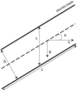
Used with permission. . . 7 2-2 Simplied diagram depicting blade geometry parameters. . . 9 2-3 Example blade camber line used to illustrate the relationship between

cosκ and |nˆθ|. . . 10

2-4 One iteration of the extraction process [1]. Used with permission. . 11

3-1 Process conducted during automated body force model development. 18 3-2 Rotational and non-rotational sections of the NASA Rotor 67 hub [18]. 20 3-3 Single Passage rotor (left) and stator (right) grid topologies at midspan

[1]. Flow is from left to right. . . 22 3-4 Single-passage domain as dened in CFX-Pre [1]. . . 23 3-5 Meridional view of body force grid. (a) Complete computational

do-main; (b) rotor swept volume; (c) stator swept volume. . . 24 3-6 Flow chart depicting the incorporation of the user's body force grid. 25 3-7 Single stage schematic displaying positive and negative blade mean

camber angles. . . 27 3-8 Flow chart depicting the compressibility correction loop. . . 31 3-9 Mismatched swirl velocity with a constrained ow angle due to absence

3-10 Process conducted during optimization of parallel force model coe-cients at ow coecoe-cients either above or below peak eciency. . . 36 3-11 Example Nelder-Mead process for two variable optimization [21]. . . . 39 3-12 Exchanging of coecients between parallel optimization processes. . . 41 4-1 Automated model versus user-generated model for ow angle deviation

from single passage. (a): rotor; (b): stator. . . 44 4-2 Comparison of work coecient between single passage and body force

results. . . 45 4-3 Objective function history for rotor viscous force coecients

optimiza-tion. . . 46 4-4 Objective function history of stator viscous force coecients

optimiza-tion. . . 48 4-5 Body force speedline of isentropic rotor and stage eciency compared

with single passage results. . . 50 4-6 Rotor total temperature ratio, total pressure ratio, and stage total

List of Tables

3.1 Important design characteristics for NASA Rotor 67 at 90% speed [18, 19]. . . 19 3.2 Grid count statistics for both single passage and full annulus RANS

calculations[1]. . . 22 3.3 Body force grid independence study. . . 24 4.1 Outputs of the normal force and peak-eciency viscous force model

calibration. . . 43 4.2 Automated model versus single passage and Hill's model. . . 43 4.3 Operating points used during optimization procedure. . . 45 4.4 Viscous force coecients produced by Nelder-Mead optimization for

the rotor. . . 46 4.5 Viscous force coecients produced by Nelder-Mead optimization for

the stator. . . 47 4.6 Body force reported isentropic eciencies versus single passage result. 49 4.7 Computational time required for model development; computations on

Nomenclature

Symbols

AR aspect ratio B number of blades cblade chord

e specic total energy

f volumetric source term per unit mass F volumetric source term per unit volume F objective function

F P R fan/compressor pressure ratio

h enthalpy, staggered spacing in blade row Kn Peters volumetric source term coecient

˙

m mass ow rate M Mach number

ˆ

nθ circumferential projection of the local blade unit normal vector

p pressure

˙

Q rate of heat transfer r radial coordinate s blade pitch U blade speed V absolute velocity W relative velocity

˙

x, y, z Cartesian coordinates α absolute swirl angle β relative swirl angle δ ow deviation angle

compressibility correction factor η eciency

θ circumferential coordinate κ local blade camber angle

Λ re-cambering constant

ρ density σ blade solidity

υ relative grid density φ axial ow coecient ψ rotor work coecient

Ω fan rotational speed

Subscripts

BF body force in inlet

is isentropic LE leading edge maxmaximum min minimum

n direction normal to streamline out outlet

p direction perpendicular to streamline ref reference

rel relative

SP single passage

T E trailing edge

Superscripts

M mass-averaged quantity

Abbreviations

CCL CFX Command Language CFD Computational Fluid Dynamics RANS Reynolds-Averaged Navier-Stokes RMS Root Mean Squared

Chapter 1

Introduction

non-experts by producing an automated model development system.

Figure 1-1: Body force eld in the swept volume of the actual blade row [4]. Used with permission.

1.1 Objective and High-Level Approach

1.2 Challenges

Normally the body force model calibration process involves the use of several software packages and users manually move data between these tools. Therefore, automated data interchange and minimizing the movement of data between software packages are important challenges to address. Another obstacle faced when developing the automated system is determining when the model is suciently accurate. This in-volves specifying convergence criteria for each of the iteratively-determined aspects of the modelling approach. Setting the values for the convergence criteria is done with reference to previously conducted work on the same turbomachine used for de-velopment in this thesis [1]. The nal challenge faced during system dede-velopment is the generalization of the approach to account for any blade row. This challenge involves converting hard-coded parameters for the machine used during this study to functions capable of accepting user input for the machine of interest.

1.3 Major Findings and Conclusions

blade row. Following the user input, the system is suciently robust to extract all relevant data provided by the user and incorporate it into the models of both the viscous and turning forces.

1.4 Thesis Outline

Chapter 2

Literature Review

This chapter details the state of the art with regard to existing expert systems, opti-mization processes where an analytical version of the objective function is unknown, and body force modelling methodology. The expected contribution of the thesis is also outlined.

2.1 Body force modelling

Body force modelling was introduced by Marble[2] as replacing the physical blade row by an innite number of innitely-thin blades. The body forces are then broken down into a normal force per unit mass, fn, and parallel force per unit mass, fp.

The normal force acts perpendicular to the relative streamlines, working to reduce the deviation of the ow from the blade camber surface (the locus of blade camber lines from hub to tip). The parallel force acts against the streamwise direction and generates viscous losses in the ow. These two forces are illustrated in Figure 2-1.

implementation are: ∂ ∂t            rρ rρVx rρVr rρVθ

rρet

           = ∂ ∂x            rρVx

rρV_x2+rρ rρVxVr

rρVxVθ

rVx(ρet+p)

           + ∂ ∂r            rρVr

rρVrVx

rρV2

r +rp

rρVrVθ

rVr(ρet+p)

           + ∂ ∂θ            ρVθ

ρVθVx

ρVθVr

ρV2

θ +p

Vθ(ρet+p)

           =            0 rFx

ρV_θ2+p+rFr

−ρVrVθ+rFθ

r

~

F ·V~ + ˙Q            , (2.1)

where the force per unit volume, −→F, and force per unit mass,f~, are related through

the local density,

− → F =      Fx Fθ Fr     

=ρ ~f =ρ      fx fθ fr      (2.2)

and the volumetric energy source term is

˙

W =ρ−→f ·−→V + ˙Q (2.3)

If the ow is considered to be adiabatic (_Q˙ _{= 0),}

˙

W ==ρfθΩr, (2.4)

whereρ is the local density, r is the radial coordinate,V~ is the absolute velocity,pis

the static pressure, Ωis the rotational speed, e is the specic total energy, and Q˙ is

circumferential blade velocity, Ωr. At each spatial location within a blade row, the

rate of total enthalpy rise per unit volume is given by Equation 2.4. If the reader desires a detailed description of the development of the current state of the art in body force modelling, Hill's recent thesis provides an excellent overview as of early 2017 [1]. In particular, see Section 2.4 of Hill's thesis. In the remainder of this section only work directly applicable to the current thesis is discussed.

Figure 2-1: Body force terms: normal turning force and parallel viscous force [4]. Used with permission.

fp =

Kp1

h "

(MM_rel)2+Kp2(M

M

rel−Mref)2

#

W2, (2.5)

where Kp1 and Kp2 are viscous force coecients, M

M

rel is the mass averaged relative

Mach number at the blade row inlet, andMref is the value ofM M

rel at peak eciency,

W is the local relative velocity, and h is the staggered blade spacing,

h= 2πr

√ σcosκ

B . (2.6)

Hereκ is the local blade camber angle,B is the number of blades, andσ is the blade

solidity,

σ= c

s, (2.7)

wherecis the blade chord length andsis the blade pitch. This formulation produces

the desired quadratic loss prole associated with turbomachines. A diagram depicting

h, κ, c, and s can be found in Figure 2-2. Peters' model is calibrated for a specic

rotational speed, which produces a speedline for varying ow coecient. The term `speedline' refers to a performance assessment across a range of operating conditions, using performance metrics such as the isentropic eciency, total pressure ratio, or total temperature ratio. Varying the rotational speed would require updated model calibration constants.

Figure 2-2: Simplied diagram depicting blade geometry parameters.

An incompressible, inviscid body force model was developed by Hall et al.[5]. The inviscid assumption eliminates the need for a viscous model. The normal force model is a function of local ow quantities and blade camber angle, allowing the model to be formulated without the need of a single passage RANS calculation for calibration. The normal force per unit mass is expressed as

fn=

(2πδ) 1₂W2_/|nˆ

θ|

2πr/B , (2.8)

wherenˆθ is the circumferential projection of the local blade unit normal vector and δ

is the local deviation angle. However, this approach is limited by the fact that there is no mechanism to model the eects of blade metal blockage and that it only yields accurate models in low-speed ows, due to its assumption of incompressible ow.

developed at the University of Windsor by Hill[1] are added to Hall's normal force modelling approach. An addition to the deviation term () captures compressibility

eects by matching the relative ow angles produced by the body force model with those reported from circumferential averages of single passage simulations:

fn =

2π(δ+)1₂W2

2πr|nˆθ|/B

fn =

(δ+)W2

2rcosκ/B. (2.9)

where the substitution |nˆθ| = cosκ has been made; this trigonometric relationship

can be visualized in Figure 2-3.

Figure 2-3: Example blade camber line used to illustrate the relationship between

cosκ and |ˆnθ|.

The compressibility correction is an iteratively determined spatially-varying func-tion that alters the local blade angle for the rotor and stator so that the local normal force is adjusted appropriately. Hall's normal force model, Equation 2.8, is simulated at peak eciency for the rotational speed of interest, and the relative ow angles are extracted from the results within the rotor domain in the x−r plane. These

correct work is done on the ow by the rotor. The importance of this modication can be seen from the Euler turbine equation,

ht,out−ht,in = Ω(routVθ,out−rinVθ,in), (2.10)

where ht is the total enthalpy, Vθ is the absolute-frame swirl velocity, and r is the

radial coordinate. For the body force model to produce the same total enthalpy rise as the single-passage computations, the Euler turbine equation makes it clear that the absolute swirl velocities at rotor outlet must match assuming the upstream ows are the same. This correction is necessary due to the fact that blade metal blockage is not directly modelled in the body force approach. The blade camber surface model is altered so that at the trailing edge, the correct tangential velocity is obtained. The re-camber is linearly increased from zero at the leading edge to the full amount required at the trailing edge; the implementation details are discussed in Section 3.4.6. These two changes together ensure that both leading edge incidence and trailing edge work input are correctly captured by the normal force model.

Figure 2-4: One iteration of the extraction process [1]. Used with permission.

the peak eciency Mach number. This allows for enhanced control of the eciency characteristic shape, as the quadratic slope on either side of peak eciency is not necessarily the same. The force formulation thus becomes

fp,new =

      

fp if M

M

rel < Mref0

fp

"

1 +K_p0₂M_ref0 −MM_rel

2#

if MM_rel > M_ref0

, (2.11)

where fp is Peters' loss model detailed in equation 2.5, Kp02 is a constant used to

alter the eciency at ow coecients whereMM_rel > M_ref0 . In this thesis, a simplied

version of the double-sided model is used as the parallel force model, and is outlined in Section 3.4.7.

2.2 Expert Systems

inference engine and knowledge base. Although the system presented in this thesis does not fall within the traditional denition of an expert system, it has expert sys-tem qualities, involving the application of expert knowledge (a previously-developed body force modelling approach and resultant model [1]) to obtain a body force model without the need for user interaction during model development. The knowledge base can be thought of as the level of agreement between the model and the single passage calculations, the form of the model functions, and the default number of points on the speedline used for optimization; the inference engine can be thought of as the algorithm itself.

Previously conducted research in the areas of computational uid dynamics (CFD) and automated modelling do not incorporate automated model development, but in-stead incorporate automated model selection for the user-supplied problem descrip-tion. For example, Koziel et al.[9] produced a system that selects grid and ow parameters which are typically chosen by a user while optimizing airfoil shape. De-pending on the resultant parameters, the system then chooses the best-choice CFD model for the shape of the airfoil. The main advantage of Koziel's system is the reduction in computational time when compared to conventional low-delity model development. The automated turbomachinery model development system presented in this thesis is therefore something that has not been done before.

2.3 Optimization

all of these methods provide suitable approaches when optimizing objective functions with unknown gradients, they are typically used for problems with large numbers of variables; however, the Nelder-Mead method performs best with few design variables. The genetic algorithm and particle swarm optimization procedures are considered brute force methods that require a large number of function evaluations [11]. As outlined in Section 3.4.7, the number of variables being optimized in this thesis is two. This suggests the Nelder-Mead method is the best optimization method for this problem.

The Nelder-Mead method was developed by J. A. Nelder and R. Mead. The method minimizes a function of n variables, which depends on the comparison of

function values at the n+ 1vertices of a general simplex, followed by the replacement

of the vertex with the highest value by a new vertex. A simplex is a structure in n

-dimensional space formed byn+1points that are not in the same plane. For example,

2.4 State of the Art and Limitations of Previous

Re-search

When developing a body force model, the current state of the art requires a user to manually develop the model. This involves tuning the model constants, as well as post-processing the model results; to conduct these steps eectively, signicant user expertise is required. Eliminating the need for user expertise can be achieved through the use of an automated system. The viscous model development that is typically conducted by tuning the model coecients could instead by subjected to an optimization process, specically the Nelder-Mead method. To the author's knowledge, no work has been conducted to produce an automated expert system with these capabilities.

Chapter 3

Approach

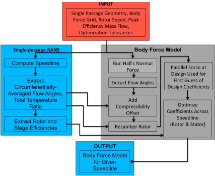
Typically, the models described in Section 2.1 require signicant user experience to calibrate, and the processing of data produced by the model and the higher-delity single passage computations required for calibration is also a task which typically re-quires signicant user experience and eort. This chapter describes the functionality and use of an automated system that eliminates the majority of user expertise and in-teraction required to obtain a well-calibrated model. The automated system requires user input to commence model development. The input required is as follows:

ˆ single passage geometry and the grid for the blade row(s) of interest;

ˆ the corrected rotational speed of the machine, or the speed of the machine if the inlet temperature corresponded with ambient conditions at sea level; ˆ the peak-eciency corrected mass ow rate of the machine at the given corrected

speed;

ˆ the operating points chosen for the speedline of interest; and

ˆ the tolerance for convergence of the objective function and the variables being optimized related to the viscous force coecients.

OUTPUT INPUT

Single-passage RANS Body Force Model

Single Passage Geometry, Body Force Grid, Rotor Speed, Peak

Efficiency Mass Flow, Op>miza>on Tolerances

Compute Speedline

Extract Circumferentially- Averaged Flow Angles,

Total Temperature Ratio

Run Hall’s Normal Force

Body Force Model for Given Speedline Extract Rotor and

Stage Efficiencies

Extract Flow Angles

Add Compressibility

Offset

Recamber Rotor

Parallel Force at Design Used for First Guess of Design Coefficients

Op>mize Coefficients Across

Speedline (Rotor & Stator)

Figure 3-1: Process conducted during automated body force model development.

3.1 Machine Used for Assessment

typical compressor. This means that the ow response is similar to that of a rst stage compressor or a low bypass ratio fan in a turbofan engine.

Table 3.1: Important design characteristics for NASA Rotor 67 at 90% speed [18, 19].

Ω (rad/s) 1512 σhub 3.11

Mrel,tip 1.20 σtip 1.29

FPR 1.48 rhub

rtip

inlet 0.375

˙

m (kg/s) 31.10 rhub

rtip

outlet 0.478

B 22 ηis(%) 92.2

AR 1.56 φ = VxM

Umid 0.50

tip clearance

rtip (%) 0.39

,

In the table, FPR is the fan pressure ratio, σ is the blade solidity, ηis is the rotor

isentropic eciency, m˙ is the mass ow rate, AR is the rotor blade aspect ratio, and

φis the ow coecient. The rotor consists of 22 blades which rotate clockwise (facing

Figure 3-2: Rotational and non-rotational sections of the NASA Rotor 67 hub [18].

3.2 Single Passage Computations

por-tion of the grid was created using Pointwise [17], while the remaining secpor-tions of the grid were created using ANSYS TurboGrid [20]. Due to the complexity of the grid near the physical blade, TurboGrid is the preferred software as it uses an automated grid generation algorithm, catered towards the study of turbomachinery. The NASA stage 67 rotor has a large stagger angle near the blade tip, and due to this stagger, the complexity of the grid is signicantly increased in the outer span regions. For this reason, TurboGrid is especially useful in comparison to manual grid generation. A further advantage of TurboGrid is its handling of a non-conformal tip gap, as the rotor region requires a tip gap of 0.0039Rtip to allow rotor clearance while

operat-ing [1]. For a more detailed description of the soperat-ingle passage grid generation, please see Section 3.3.2 of Hill's thesis. Table 3.2 outlines grid count statistics, where the relative grid density,υ, is calculated as

υ = Cell%

Volume%. (3.1)

The Spalart-Almaras turbulence model is used with y+ _{<30. The boundary}

con-ditions are stagnation pressure and temperature at inlet and mass ow rate specied at outlet. Mixing planes are incorporated upstream and downstream of the rotor, or alternatively only between the rotor and stator. The convergence criterion is a con-servation target for mass, momentum, and energy ux of <0.5% and RMS residuals

< 1.0×10−3. An illustration of the single passage computational domain used for

Table 3.2: Grid count statistics for both single passage and full annulus RANS calculations[1].

Region Cell/Passage Passage/360◦ Cells/360◦ Volume % Cell % υ

Inlet 458,346 22 10,083,612 52.9 10.5 0.198 Rotor Inlet 106,848 22 2,350,656 8.42 2.44 0.290 Rotor 1,781,061 22 39,183,342 6.04 40.8 6.75 Stator 1,065,792 36 38,368,512 4.29 39.9 9.30 Outlet 171,600 36 6,177,600 28.4 6.42 0.226

Total 3,583,647 96,163,722

Figure 3-4: Single-passage domain as dened in CFX-Pre [1].

3.3 Body Force Grid Generation

is recommended.

(b) (c)

(a)

Figure 3-5: Meridional view of body force grid. (a) Complete computational domain; (b) rotor swept volume; (c) stator swept volume.

Grid independence is conrmed at 90% corrected speed; Table 3.3 quanties the changes between a baseline and ne grid. The parameters used to monitor grid independence are the isentropic rotor eciency, and the rotor work coecient

ψ = ∆ht

U2 , (3.2)

where ∆ht is the rise in total enthalpy across the rotor and U is the blade tip speed.

The changes in both parameters are small enough that the baseline grid is suciently ne.

Table 3.3: Body force grid independence study.

Baseline grid Fine grid % Change Cell count 5.25×104 1.45×105 176%

Rotor work coecient 0.2248 0.2263 0.67% Rotor isentropic eciency 87.32% 87.46% 0.16%

3.4 Body Force Model Calibration

com-3.4.1 Incorporation of User-Provided Body Force Grid

The rst automated step in the system is the input of the user's body force grid. A ow chart depicting the high-level process conducted during this step in the automated procedure can be seen in Figure 3-6.

Matlab Working Environment

User’s Body

Force Grid Input User Grid Into Body Force .def file

CFX

Simulate 1 iteraEon with new grid

CFD Post: Export Rotor and Stator grid

points to .csv file Read grid data into

Matlab workspace

Write session files containing body force grid points in

user funcEons

Figure 3-6: Flow chart depicting the incorporation of the user's body force grid.

(detailed in Section 2.1) is conducted at the specic points in the computational do-main corresponding with the body force grid points, which is why accurate knowledge of these points is needed. A ow simulation on the body force grid, with no model present for the blade rows (so, an empty duct) is run for one iteration to initialize the axial and radial coordinates of the body force grid points in the results le that is needed for post-processing of the single-passage computations. A CFD-Post session le writes the coordinates of the grid points to a .csv le, which is then read into the Matlab script responsible for the automation. CFX-Pre and CFD-Post session les are then created using Matlab's fprintf command by appending the body force grid points to an already existing segment of the session les. These CFD-Post session les are responsible for the extraction of the single passage circumferentially averaged ow angles, body force circumferentially average ow angles, and the body force model's compressibility correction () at the specic body force grid points. The CFX-Pre

session le is used to input the newest version of the compressibility correction at the correct spatial location during model calibration iterations.

3.4.2 Generation of Blade Geometry Fields for Each Blade

Row

The 3D blade data corresponding with the single passage geometry is used to generate blade geometry elds, a required input for the body force computations. The axial and radial coordinates, as well as the corresponding local blade mean camber angle from the meridional direction (κ) are needed. The format of the data for the rotor

x_s and provided in metres, the radial coordinate should be in a variable named r_s and provided in metres, and the local blade mean camber angle should be in a variable named kappa_s and provided in degrees. These three sets of data should be compiled in a Matlab .mat le, and stored in the working directory of the automation script. The local blade mean camber angle is dened to be negative in the direction of rotor rotation and positive opposite the direction of rotor rotation (so generally in the rotor the angles will be positive while in the stator they will generally be negative). The schematic found in Figure 3-7 illustrates positive and negative blade mean camber angle conventions.

Figure 3-7: Single stage schematic displaying positive and negative blade mean cam-ber angles.

This data is then interpolated onto the body force grid points within the script re-sponsible for the automation procedure via Matlab's scatteredInterpolant function. The blade mean camber angle along with its axial and radial coordinates are used to create the interpolant function, and the body force grid points' axial and radial coordinates are used as the query points for the interpolation. Linear interpolation is used. The interpolated data is used to create elds forκ, σ,h,κT E, andκLE for each

blade row, whereκT E, and κLE are the blade mean camber angle at trailing edge and

3.4.3 Single Passage Computations

Prior to commencing the body force model calibration, the data used for that cal-ibration is needed. Thus single passage computations are conducted, in series, at all user-specied operating points. CFX-Pre session les are created using Matlab's fprintf command for the purpose of creating case denition .def les for all of the operating points chosen. The .def les are created using Matlab's system command to run the session les previously mentioned. The simulations are conducted via Mat-lab's system command by utilizing CFX's command line capabilities. This process starts at the operating point corresponding with the highest ow coecient, and upon achieving a converged solution moves to the next operating point on the speedline (reducing ow coecient). The results le from the most recently simulated operating point is used to initialize each of the remaining simulations to decrease computational cost.

3.4.4 Initial Body Force Computations

Turning force model calibration begins with a rst body force simulation at the peak eciency operating point with a simplied viscous force model present. The turning force model at this stage in the process is Hill's model without the compressibility correction (equivalent to Hall's model):

fn =

(δ)W2

2rcosκ/B, (3.3)

while the viscous force model at this stage in the process is expressed as

fp =

K_p∗ h

MM_rel2W2, (3.4)

with W representing the relative velocity for the rotor. Note that in the stator's

parallel force model, absolute velocity V is used instead ofW. For the initial

compu-tation, an empirical guess forK_p∗ is used,K_p∗ = 0.0145in the rotor andK_p∗ = 0.052in

the stator. These empirical predictions were the nal values discovered by Hill during his research [1]. The simulation is conducted in parallel across 3 cores. During system development, it was found that this level of parallelization produced the fastest results for the body force grid used. Flow angles (relative in rotor, absolute in stator) are computed from the results with a CFD-Post session le, and the dierence from the corresponding single passage reported angles is computed within the session le using Perl commands. The dierence is computed at all body force grid locations within the blade row(s), and sets the rst version 1 of the compressibility oset correction

.

1,rotor(x, r) =βSP (x, r)−βBF(x, r), (3.5)

1,stator(x, r) =αSP(x, r)−αBF (x, r), (3.6)

where βSP (x, r) is the relative circumferentially-averaged ow angle in the rotor

reported from the body force computation,αSP (x, r)is the absolute

circumferentially-averaged ow angle in the stator reported from the single passage results, andαBF (x, r)

is the absolute ow angle from the stator reported from the body force computation. The session le writes the compressibility correction data at all grid locations to a .txt le along with the axial and radial coordinates of the corresponding grid point, which is stored within the working directory. Within this same session le, the dif-ference in isentropic rotor and stage eciencyη between the body force computation

and the single passage results is used for a calculation of the update of the viscous force coecient K_p∗ in both the rotor and stator, respectively, which is written as

a .txt le and stored within the working directory. The dierence between the two eciencies sets the value for a viscous force coecient incorporated in the denition of the viscous force as seen in Equation 3.7. At this point in the process it is expected that the dierence between the two eciencies is small enough so that K_p∗ will scale

linearly:

K_p∗ =

1− ηSP −ηBF ηSP

K_p∗

empirical. (3.7)

Following the rst iteration ofK_p∗, the eciency dierence acts as a scaling factor on

the previous K_p∗ value, as seen in Equation 3.9.

3.4.5 Determining the Final Compressibility Correction

First version of ε, and Kp*

Current version of ε, and Kp* input into body force .def file

Body force simula=on run un=l convergence

Flow angle difference, as well as isentropic efficiency difference set updated versions

of ε, and Kp*

Do both loop monitors indicate process is complete?

No Yes

Loop con=nues

Process moves to next segment

Compressibility Correc=on Loop

Figure 3-8: Flow chart depicting the compressibility correction loop.

To start, a CFX-Pre session le reads the .txt le pertaining to the current version of the compressibility correction elds i and Kp∗ (for the rotor and stator) via Perl

scripting commands. The session le then inputs the data into the body force .def le via CCL. The simulation at the peak eciency corrected mass ow is initialized from the most recent body force results le and run to convergence. The dierence between the body force and single passage results is assessed within the same CFD-Post session le detailed in Section 3.4.4, and sets the updated versions of and K_p∗

as follows:

new(x, r) =old(x, r) +

"

βSP (x, r)−βBF (x, r)

#

K_p,new∗ =     

K_p,old∗ 1−Cemp

q

ηBF−ηSP

ηSP

ifηBF ≥ηSP

K_p,old∗

1 +Cemp

q

ηSP−ηBF

ηSP

ifηSP > ηBF

, (3.9)

whereCempis an empirical scaling factor set to 0.225 and 0.45 for the rotor and stator,

respectively. These values come from Hill's research, and are based on the iterative procedure he conducted while manually adjustingK_p∗ [1]. AsηBF approachesηSP, the

adjustment of K_p∗ based on the eciency alone typically results in over-adjustment,

thus Cemp is incorporated to reduce overshoot ofKp∗. The while loop implemented

in Matlab repeats this process until monitors for the rate of change of both quantities determine that the model is converged. The details of these monitors M are as

follows:

M(x, r) =

i(x, r)

i−1(x, r)

−1 (3.10)

MKp =

|ηSP −ηBF|

ηSP

. (3.11)

The compressibility correction monitor is evaluated at all body force grid points, and the maximum value is used for the nal assessment. Convergence is achieved when both of these monitors fall below 0.01. This value is chosen as it signies that the body force model is within 1%agreement with the single passage isentropic eciency

results, which is deemed suciently accurate by the author. For the compressibility correction, this represents a maximum change at all body force grid points of 1%,

suggesting the ow angles are suciently matched.

3.4.6 Rotor Blade Recambering

the trailing edge work input, the model incorporates Hill's recambering process [1]. Prior to commencing this process, a CFD-Post session le is used to extract the mass-averaged total temperature ratio across the rotor (τ) from the body force computation

result responsible for terminating the compressibility correction loop. The dierence between the body force and single passage result for this total temperature ratio sets the rst version of a design constant to begin the rotor blade recambering process. The rst version of the recambering constant scales linearly with an empirical recambering constant of Λempirical = 0.27, which was the version of the constant found by Hill

during his research [1].

Λ=

τN AT

τSP

Λempircal (3.12)

A while loop implemented in the Matlab script responsible for model calibration starts by using a CFX-Pre session le to input the current version of the recambering design constant into the body force .def le. This aects the blade camber distribution as follows:

κnew(x, r) = κold(x, r) +Λrecamber

(x−xLE(r))

(xT E(r)−xLE(r))

(βT E,SP(r)−βLE,SP(r)),

(3.13) whereκnew(x, r)is the new blade camber prole at each rotor grid point. A schematic

produced by Hill details the eect of recambering [1], and can be seen in Figure 3-9. Typically the blade loading is highest in the rst quarter chord of the rotor blade, thus the recambering is performed linearly from leading edge to trailing edge, meaning that the camberline is unaltered at the leading edge. By linearly recambering, the body force camberline is a combination of correct swirl angle at the leading edge and correct swirl velocity at the trailing edge. To produce the recambered blade, changes in relative ow angle from leading edge to trailing edge are extracted from single passage RANS and are used to radially scale the re-cambering, as seen in Equation 3.13 represented by the (βT E,SP (r)−βLE,SP(r)) term. By doing this, the spanwise

obtained. Following the input of the recamber constant, the rst recamber simulation is initialized by the most recent body force results le and run to convergence. A CFD-Post session le extracts the total temperature ratio previously discussed and this is used to compute a new value of the recambering constant as follows:

Λnew =

     Λold

1−q1− τBF

τSP

if τSP ≥τBF

Λold

1 +qτBF

τSP −1

if τBF > τSP

. (3.14)

In a similar manner to the compressibility correction loop, the recambering loop makes use of a convergence monitor. The details of the monitor is as follows:

Mrecamber =

1− τBF τSP . (3.15)

The monitor terminates the loop if the calculation results in a value equal to or less than 0.01. This value is chosen as it signies that the body force model is within

1% agreement with the single passage rotor total temperature ratio, which is deemed

Figure 3-9: Mismatched swirl velocity with a constrained ow angle due to absence of blockage [1]. Used with permission.

3.4.7 Viscous Force Coecient Optimization

With the normal force model complete, the automation scheme begins the calibration of the parallel force model. The parallel force model used in this thesis is a modied version of Hill's model [1], which can be found in Equation 2.11. The form of the viscous force model used in this work can be seen in Equation 3.16.

fp =

       Kp1 h

MM_rel

2

+Kp2

MM_rel−Mref

2

W2 if_MM

rel ≤M M rel, peakη Kp10

h

MM_rel2+K_p0₂MM_rel−M_ref0 2

W2 _ifMM

rel > M M rel, peakη

where the primed coecients denote the viscous coecients used above the peak e-ciency point, and the non-primed coecients are used below the peak ee-ciency point. In isolating the parallel force model above the peak eciency point from the model below the peak eciency point, the two models can be solved for simultaneously, as the coecients are independent. As mentioned in Section 2.1, typically the coe-cients Kp1,Kp2, andMref are adjusted in attempts to match the eciencies reported

by the model at all operating points along the speedline. However, in this automated model calibration, the viscous force coecients are subjected to a Nelder-Mead op-timization procedure implemented in Matlab via the fminsearch algorithm. The process is illustrated in Figure 3-10.

First guess of coefficients

Current version of coefficients input into .def files at all

opera7ng points

Simula7on at all opera7ng points with current version of coefficients un7l convergence

Isentropic efficiency extracted from body force results files at

all opera7ng points

Objec7ve func7on evaluated. Is value the minimum?

No Yes

Algorithm adjusts coefficients

Op7mized parallel force model

Objec7ve Func7on

The objective function for the optimization process is

Fobj =

s Pn

i=1(ηSP −ηBF) 2

n , (3.17)

wheren is the number of operating points (including peak eciency) on a given side

of peak eciency. The objective function for the rotor is the RMS error between body force and single passage reported rotor isentropic eciency, while the stator's objective function is the RMS error of the stage isentropic eciency. Because the rotor has a direct eect on the stage eciency, it is important to optimize the model for the rotor prior to that of the stator. The completion of the previously conducted compressibility correction loop indicates that the simplied fp at the peak eciency

operating point corresponds with sucient agreement between the single passage and body force isentropic eciences. Rearranging Equation 3.4 leads to

K_p∗ = fp

MM_rel2W2

h. (3.18)

Rearranging Equation 3.16 leads to Kp1 expressed as

Kp1 =

fp

MM_rel

2

+Kp2

MM_rel−Mref

2 W2

h, (3.19)

eectively reducing the number of independent variables from 3 to 2 (Kp2 andMref).

The rst guess for Mref is simply M M

rel, which is consistent with the rst guess Hill

employed during his study [1]. This reduces Equation 3.19 to

Kp1 =

fp

MM_rel2

W2

h=K_p∗ (3.20)

A CFD-Post session le is used to extract K_p∗ from the body force results le upon

the ratio of Hill's nal versions of Kp1 and Kp2 to set the guess as

Kp2 = 40000Kp1. (3.21)

Upon being subjected to the rst guess

~xo = [Kp2 Mref], (3.22)

the fminsearch algorithm creates a simplex around this guess by adding 5% to each component of~x0 to create two new vectors. The algorithm uses these two new vectors

Figure 3-11: Example Nelder-Mead process for two variable optimization [21].

Following the rst guess, the main script calls a second instance of Matlab. The two scripts run in parallel to simultaneously solve the optimization problems above and below the peak eciency point. The two optimizations are independent and are carried out in parallel to reduce the time required for model calibration. The system optimizes the rotor coecients rst, and upon completion, optimizes the stator coecients using the same approach.

corresponding operating point. Upon reaching a converged solution, a CFD-Post session le extracts the relevant isentropic eciency, and writes the value of the eciency to a .txt le stored within the working directory. Once the eciency at all operating points is obtained, the values are read into the working directory and the objective function is evaluated. Each iteration of the optimization procedure records the version of the coecients being optimized, as well as the corresponding value of the objective function into a plain text le so that convergence can be externally monitored. Before moving to the next iteration of the optimization procedure, the optimization below the peak eciency reads the latest version of the viscous force coecients above peak eciency, and inputs these into the body force .def le below peak. The same is done vice-versa above the peak eciency point, to ensure that upon completion, the model is complete (both above and below peak eciency point coecients will be correct). A visual representation of the exchange of coecients between the above and below peak eciency optimization procedures is presented in Figure 3-12.

Op#miza#on Above Peak Efficiency Opera#ng Point Op#miza#on Below Peak

Efficiency Opera#ng Point

Input of coefficients Input of coefficients

Simulate all opera#ng points

Evaluate objec#ve func#on

Write current version of coefficients

Simulate all opera#ng points

Evaluate objec#ve func#on

Write current version of coefficients

Read other side’s

coefficients Read other side’s coefficients

Working Directory

Chapter 4

Body Force Model Assessment

In this chapter, the body force model produced by the automated system for NASA stage 67 at 90% corrected design speed is detailed. The model's performance is assessed with comparison to single passage results, as well as the results produced by Hill's manually generated body force model [1]. The results of the viscous force optimization for both the rotor and stator is presented, as well as the associated computational cost of model calibration.

4.1 Normal Force and Peak-Eciency Viscous Force

Model

Table 4.1: Outputs of the normal force and peak-eciency viscous force model cali-bration.

K_p,rotor∗ K_p,stator∗ Λ

Constant 0.0209 0.109 0.204 # of Iterations 22 2

At the peak eciency mass ow rate, 31.1 kg/s (ow coecient φ = 0.5 based

on midspan blade speed), the relevant results produced by the normal force model are outlined in Table 4.2. The model's results are compared with the single passage counterparts, and the results produced by Hill's work [1], with the error calculated relative to the single passage results.

Table 4.2: Automated model versus single passage and Hill's model.

single passage automated model % error Hill's model % error

˙

mcorr (kg/s) 31.1 31.1 31.1

ηis(rotor, %) 92.5 93.2 0.75 92.4 0.10

ηis(stator, %) 89.3 90.1 0.84 90.0 0.79

τrotor−1 0.1291 0.1294 0.23 0.1314 1.78

The agreement between the automated model and the single passage results is on par with Hill's results, except for the rotor isentropic eciency. This can be attributed to the monitor responsible for K_p,rotor∗ , seen in Equation 3.11, as the percent error

fell below the 1% threshold corresponding with loop convergence. If the user of the

automated system desired a stronger agreement, adjusting the convergence criteria accordingly for Equation 3.11 would accomplish this.

The nal version of the compressibility correction, , is obtained in the same

loop used to determine, K_p∗, as outlined in Subsection 3.4.5. Hill's model required

19 iterations to obtain the nal spatial eld [1], whereas the automated model

4-1. This gure indicates that the automated model produces stronger matching between the single passage and body force reported ow angles than does the user-calibrated approach. As mentioned in Section 3.4.5, the process of determining the compressibility correction,, involves observing the change inbetween each iteration.

This result suggests that the convergence criteria for the compressibility correction monitor, Equation 3.10, is more precise than the traditional manual method.

Figure 4-1: Automated model versus user-generated model for ow angle deviation from single passage. (a): rotor; (b): stator.

Figure 4-2: Comparison of work coecient between single passage and body force results.

4.2 Viscous Force Coecient Optimization

The operating points chosen for this study are outlined in Table 4.3. These points were chosen as they correspond with evenly distributed locations on the speedline being simulated, centred around the peak eciency operating point of 31.1 kg/s.

Table 4.3: Operating points used during optimization procedure. Operating Point 1 2 3 4 5 6 7

˙

mcorr (kg/s) 28.7 29.5 30.3 31.1 31.9 32.7 33.5

φ 0.461 0.474 0.487 0.5 0.513 0.526 0.539

required 41 iterations of the Nelder-Mead optimization algorithm, and the conver-gence history of the objective function can be found in Figure 4-3. The RMS error minima determined for the rotor optimization procedure is 0.0099 and 0.0017 for below and above peak respectively.

Table 4.4: Viscous force coecients produced by Nelder-Mead optimization for the rotor.

Below Peak Above Peak

Kp1 0.003467 Kp01 0.01157

Kp2 660.5 Kp02 662.5

Mref 1.061 Mref0 0.9620

MM_{rel, peakη} 0.9870 MM_{rel, peakη} 0.9870

stator's viscous force coecients are optimized in an identical manner. The coe-cients produced by the Nelder-Mead optimization can be found in Table 4.5. These coecients were obtained following 27 and 32 iterations for below and above the peak eciency point respectively, and the convergence history for the optimization process can be found in Figure 4-4. The RMS error minima determined for the stator opti-mization procedure is 0.0517 and 0.0897 for below and above the peak eciency point respectively. Comparing these minima with those found for the rotor's optimization process suggests that the stage eciency may not be the most suitable parameter to calibrate the stator's viscous force model. Further discussion of this nding can be found in Section 5.3.

Table 4.5: Viscous force coecients produced by Nelder-Mead optimization for the stator.

Below Peak Above Peak

Kp1 0.00108 Kp01 0.05062

Kp2 12.92 Kp02 5.606

Mref 1.761 Mref0 0.6492

Figure 4-4: Objective function history of stator viscous force coecients optimization.

The eciency as a function of ow coecient produced by the model is compared with the single passage results used for calibration in Figure 4-5. As the RMS error minima suggests, the stator's viscous force model does not produce the same level of agreement as the rotor's viscous force model. The model is unable to match the steep decline in stage eciency as the operating conditions move away from the peak eciency operating point. The isentropic eciencies produced by the body force model are compared at each operating condition to the single passage result used for calibration in Table 4.6. The model predicts the rotor isentropic eciency suciently well, with the highest error being1.32%, and the smallest being0.10%. The model is

coecients is low in comparison to the rotor results. The single passage results at the two highest mass ows are nearing choke conditions, and the lack of blade metal blockage in the body force model becomes more signicant, as the results in Table 4.6 suggest. Possible solutions are outlined in Section 5.3.

Table 4.6: Body force reported isentropic eciencies versus single passage result.

˙

mcorr (kg/s) 28.7 29.5 30.3 31.1 31.9 32.7 33.5

ηrotor,BF (%) 89.4 91.1 92.3 92.7 91.5 88.9 84.3

ηrotor,SP (%) 89.0 90.0 91.2 92.5 91.7 88.8 84.2

% error 0.506 1.16 1.32 0.227 0.240 0.101 0.131

ηstage,BF (%) 86.0 88.3 90.4 90.6 88.9 85.7 80.1

ηstage,SP (%) 77.7 82.8 88.0 89.3 87.9 77.3 64.4

Figure 4-5: Body force speedline of isentropic rotor and stage eciency compared with single passage results.

Figure 4-6: Rotor total temperature ratio, total pressure ratio, and stage total pres-sure ratio at o-design conditions.

4.3 Computational Cost

Model calibration requires numerous iterations for each step of the process. The computational cost of each step is outlined in Table 4.7, with the computational time being presented in terms of core-days. Model calibration was conducted on an Advanced Clustering Technologies MicroHPC2_{Workstation [21], which contains two}

is that the simulations conducted during stator optimization converged quickly as the coecients were changing minimally between iterations.

Table 4.7: Computational time required for model development; computations on 3 cores @ 1.7 GHz.

Step of Model Calibration # of Iterations Computational Time (core-days) Compressibility Correction 22 11.5

Rotor Recambering 2 0.5

Rotor Optimization Below Peak 41 10.0 Rotor Optimization Above Peak 41 10.0 Stator Optimization Below Peak 27 1.0 Stator Optimization Above Peak 32 1.0

Full Model Development 23.0

Chapter 5

Conclusions and Future Work

In this thesis, an automated system is presented for the purpose of calibrating a body force model for a single stage compressor. In this chapter, a summary of the work conducted, the key ndings of the study, and recommendations for future work are discussed.

5.1 Summary

In the past, several authors have conducted studies on the development of body force models and assessed those models' accuracy. Multiple applications of expert systems, as well as Nelder-Mead optimization procedures have been conducted in previous work; however, none of them incorporate all of these ideas at once. The lack of an existing automated system capable of producing an optimized body force model is the motivation behind the work in this thesis.

adaptation of Peters' model, applying two unique instances of the model on either side of the peak eciency point. The automated system is implemented in Matlab, using CFX-Pre and CFD-Post session les for data input and output respectively.

The model is able to produce results at the peak eciency operating point to within 1% of the single passage results for both work input and eciency. At this oper-ating condition, the automated model performs almost identically to a user-generated model produced in Hill's work. The portion of the normal force model calibration that determines the compressibility correction results in non-physical work removal near the casing-leading edge region of the rotor. The minima found for the rotor's viscous force objective function during optimization are 0.0099 and 0.0017 for the below and above peak eciency point respectively; the minima found for the stator's viscous force objective function during optimization are 0.0517 and 0.0897 for the be-low and above peak, eciency point, respectively. The at behaviour seen in Figure 4-4 indicates that the adjustment of the parallel force coecients results in minimal change in the isentropic stage eciency produced by the model. This suggests that the stage isentropic eciency is not the most suitable parameter used to calibrate the stator's parallel force model; alternative parameters are outlined in Section 5.3. Despite this nding, the model produced performs suitably at o-design conditions not pertaining to choke conditions, predicting the rotor total pressure ratio and total temperature ratio to within0.4%and 0.2% of single passage results, respectively, and

the stage total pressure ratio to within 1.4%. This conrms the model is a

produced by this thesis is the removal of nearly all required user interaction during model calibration.

5.2 Conclusions

5.3 Potential Future Improvements

While determining the compressibility correction is necessary in the normal force model calibration, it also has a detrimental eect on the model's ability to produce accurate chordwise blade loading. The latter is desirable in terms of aeromechanical forced response prediction, as accurate predictions of the spanwise and chordwise loading distributions are crucial aspects of the modal response of the blades. In the current modelling approach, the geometric parameters outlined in Section 3.4.2 are expressed as a function of span fraction. Mapping the geometric parameters as functions of both span and chord fraction could serve to reduce the eect of non-physical work removal found near the rotor's leading edge. Also, imposing constraints on the compressibility corrections to prevent work removal would serve as a method to improve this issue.

As previously mentioned, calibrating the stator blade row's parallel force model using the stage isentropic eciency results in relatively large RMS error across the speedline chosen. A potential replacement for the calibration parameter is the stator's entropy loss coecient, as it focuses on the entropy generation within the stator rather than the stage eciency's combined eect of both blade rows. Although the minima found during the rotor's optimization procedure are much lower than the stator's, another possible parameter used for calibration of the rotor's loss model could be the loss coecient.

Allowing the user to select the level of parallelization during model development is another potential improvement. Depending on the available computational resources, the wall-clock time associated with model calibration could be reduced by allowing the user to simultaneously produce speedline computations for both the single pas-sage results used for calibration, as well as the body force model used during the optimization procedure.

3.8 responsible for determining the compressibility correction.

Bibliography

[1] D. J. Hill. Compressor performance scaling in the presence of non-uniform ow. Master's thesis, University of Windsor, 2017.

[2] F. Marble. Three-dimensional ow in turbomachines. High Speed Aerodynamics and Jet Propulsion, 10:83166, 1964.

[3] Y. Gong, C.S. Tan, K.A. Gordon, and E.M. Greitzer. A computational model for short wavelength stall inception and development in multi-stage compressors. In American Society of Mechanical Engineers, editor, ASME 1998 International Gas Turbine and Aerospace Congress and Exhibition, pages V001T01A114 V001T01A114, 1998.

[4] A. Peters. Ulta-short Nacelles for Low Fan Pressure Ratio Propulsors. PhD thesis, MIT, Department of Aeronautics and Astronautics, February 2014. [5] D.K. Hall, E.M. Greitzer, and C.S. Tan. Analysis of fan stage design attributes for

boundary layer ingestion. J. Turbomach., 139:071012107101210, July 2017. American Society of Mechanical Engineers.

[6] V. Zwass. Expert system. Brittanica, 2017. Acessed on August 27th, 2017 at https://www.britannica.com/technology/expert-system.

[7] J. Seok, J. Kasa-Vubu, M. DiPietro, and A. Girard. Expert system for automated bone age determination. Expert Syst. Appl., (50):7588, 2016.

[9] S. Koziel and L. Leifsson. Mutli-level cfd-based airfoil shape optimization with automated low-delity model selection. Procedia Comput. Sci., 18:889898, 2013. [10] S. J. Wright. Optimization. Britannica, 2017. Accessed on August 27th, 2017

at https://www.britannica.com/topic/optimization.

[11] Gradient-free optimization. Online, April 2012. Accessed on August 27th, 2017 at http://adl.stanford.edu/aa222.

[12] J.A. Nelder and R. Mead. A simplex method for function minimization. Comput. J., 7:308313, 1965.

[13] T. Osgood and Y. Huang. Calibration of laser scanner and camera fusion sys-tem for intelligent vehicles using nelder-mead optimization. Meas. Sci. Technol., 24(3), March 2013.

[14] S. Abedi and F. Farhadi. Integration of cfd and nelder-mead algorithm for optimization of mocvd process in an atmospheric pressure vertical rotating disk reactor. Int. Commun. Heat Mass, 43:138145, 2013.

[15] MathWorks Inc., Natick, MA. MathWorks MATLAB Documentation, 2017a edi-tion, 2017.

[16] ANSYS Inc., Canonsburg, PA. CFX-Solver Manager User's Guide, 17.2 edition, August 2016.

[17] Pointwise Inc., Fort Worth, TX. Pointwise User's Manual, v18.0r2 edition, 2016. [18] A.J. Strazisar, J.R. Wood, M.D. Hathaway, and K.L. Suder. Laser anemometer measurements in a transonic axial-ow fan rotor. Technical report, NASA, 1989. [19] V.J. Fidalgo, C.A. Hall, and Y. Colin. A study of fan-distortion interaction

within the nasa rotor 67 transonic stage. J. Turbomach., 134(5):051011, 2012. [20] ANSYS Inc., Canonsburg, PA. ANSYS TurboGrid User's Guide, 17.2 edition,

[21] Advanced Clustering Technologies, 3148 Roanoke Rd, Kansas City, MO. Mi-croHPC Workstation, 2017.

Appendix A

Permission to Include Copyrighted Material

12/10/2017 University of Windsor Mail - Re: EXT: Figure Request

https://mail.google.com/mail/u/0/?ui=2&ik=80b3a3baef&jsver=khUFNOKniXg.en.&view=pt&msg=15f0f703b87ea5a4&search=inbo… 1/2 Matheson West <>

Re: EXT: Figure Request

Peters, Andreas (GE Aviation) <> Thu, Oct 12, 2017 at 3:15 AM

To: Matheson West <>

Hi Matheson,

Thanks for checking. Please go ahead and use figure 3-1 from my thesis.

Best,

Andreas

From: Matheson West [mailto:] Sent: Mittwoch, 11. Oktober 2017 21:52 To: Peters, Andreas (GE Aviation) <> Subject: Re: EXT: Figure Request

Hello Dr. Peters,

Thank you for granting me permission to use this figure.

Following my oral defense, my committee requested I include a figure depicting the body force model's effect of replacing the physical blade with a domain consistent with the blade row swept volume, and Figure 3-1 in your PhD Thesis does a fantastic job of doing this. I was wondering if you could grant me permission to include this figure in my thesis. Thank you!

Matheson West

On Fri, Sep 15, 2017 at 12:23 PM, Peters, Andreas (GE Aviation) <> wrote:

Hi Matheson,

No problem - go ahead.

Andreas

On 15. Sep 2017, at 17:56, Matheson West <<mailto:>> wrote:

Hello Dr. Peters,

12/10/2017 University of Windsor Mail - Figure for Thesis

https://mail.google.com/mail/u/0/?ui=2&ik=80b3a3baef&jsver=khUFNOKniXg.en.&view=pt&msg=15ec3d9ab2d33cea&search=inb… 1/3 Matheson West <>

Figure for Thesis

hill11g <> Wed, Sep 27, 2017 at 10:58 AM

To: Matheson West <>

Mat,

Yeah man, feel free to use whatever you want.

Jarrod.

Original message ---From: Matheson West <>

Date: 2017-09-27 10:47 (GMT-05:00) To: David Hill <>

Subject: Re: Figure for Thesis

Jarrod,

Thanks for all your help with everything I've done in my research thus far. I know I already asked if you would grant me permission to use Figure 3-17 from your thesis, but I was wondering if I could also use Figure 3-16 (with credit given to you of course!)? Thanks Jarrod.

Mat

On Fri, Sep 15, 2017 at 6:32 PM, <> wrote:

Mat,

The stator was from a source Dr. Defoe provided – which I think he got from his MIT colleagues.

Jarrod.

From: Matheson West [mailto:]

Sent: Friday, September 15, 2017 12:01

To: David Hill <>

Subject: Re: Figure for Thesis

Hey Jarrod,

Sorry, another quick question for you. When you got the rotor blade data from the NASA technical report, did you have to find the stator blade data from a different source? Or was both sets of data from the NASA technical report? Thanks!

Mat

Vita Auctoris

Name: Matheson Gaelen West

Place of Birth: Walkerton, Ontario, Canada

Year of Birth: 1993

Education: M.A.Sc, Mechanical Engineering University of Windsor, 2015-2017