A New Simplified DSM-to-DTM Algorithm –
dsm-to-dtm-step
Thomas, Krauß ID
DLR, German Aerospace Center, Muenchener Str. 20, 82234 Wessling; [email protected]
Abstract: In this paper we will present a simplified approach for extracting the ground level – a digital terrain model (DTM) – from the surface provided in a digital surface model (DSM). Most existing algorithms try to find the ground values in a digital surface model. Our approach works the opposite direction by detecting probable above ground areas. The main advantage of our approach is the possibility to use it with incomplete DSMs containing much no data values which can be e.g. occlusions in the calculated DSM. A smoothing or filling of such original derived DSMs will destroy much information which is very useful for deriving a ground surface from the DSM. Since the presented approach needs steep edges to detect potential high objects it will fail on smoothed and filled DSMs. After presenting the algorithm it will be applied to a test area in Salzburg and compared to a terrain model freely available from the Austrian government.
Keywords:Digital Surface Model, Digital Terrain Model, Steep edge detection
1. Introduction
For many applications a representation of the ground is needed. Such so called digital terrain models (DTMs) are the basis e.g. for water run-off simulations or extracting elevated objects from a normalized digital elevation model (nDEM). Deriving heights from photogrammetric approaches like stereo imagery from airborne or spaceborne cameras deliver the surface of the objects – so called digital surface models (DSMs). These contain beneath the visible ground all objects above the ground. To derive the ground (DTM) many approaches already exist but none of these approaches work absolutely perfect in all cases.
Already since the 1980s there is intense research on digital terrain models [1]. A DTM is in general derived from a DSM by detecting and removing all objects and filling these areas. The problem is so the detection of off-ground objects. The Classical morphological approach [2] for example just searches for each point in a DSM the lowest neighbour in a given radius around this point. Newer approaches include e.g. the geodesic dilation as described in [3] or the multi-directional slope dependent (MSD) DTM generation method by [4] which is an extension to the directional filtering concept of [5]. The Normalized Volume above Ground (NVAG) method proposed in [6] is an extension to [4] including also the volume of the objects on the scanline.
Our presented algorithm is designed for usage together with unfilled DSMs still containing occluded areas as no-data values. For processing such DSMs we simplify the approach of [4] by just taking height steps into account and ignoring all no-data areas between.
2. Materials and Methods
Our here presented DSM-to-DTM-step approach is a simplified version of many multidirectional ground detection methods like MSD [4] or NVAG [6]. These approaches are designed for detecting ground areas in filled DSMs using much sophisticated methods for discriminating slopes in a DSM from natural slopes like on hills and object-induced slopes like such from buildings or trees. In contrast we obtain unfilled DSMs from very high resolution satellite imagery like WorldView or Pléiades with ground sampling distances of about 0.5 m. In such unfilled DSMs most of the no-data regions are occlusions near steep walls.
If such DSMs get filled these occlusions often get interpolated to a soft slope which prevent ground detection algorithms to perform correctly. Our presented approach works in contrast on the unfilled DSMs just using the last valid height and skipping any no-data areas. In the case of occlusions the last valid height is the ground, the next valid height is on the roof which results in a steep step.
So the algorithm tries to remove areas of high elevated objects from a DSM starting on a steep raising edge and lasting until a mostly not so steep edge at the end.
In detail the image is processed in four (left-right, right-left, top-bottom, bottom-top) or eight (also including all diagonals) directions and each valid heighthis compared to the previous valid heighth0in this direction – just ignoring any no-data values. If the new height is more thanUpStepu higher than the old all following pixels in this line are marked as “high” until a new height lower than DownStepdbelow the old height is found. All other pixels are left “unknown”.
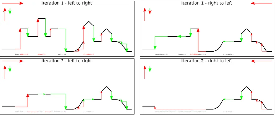
Fig.1illustrates the method. In the top row the processing of the first iteration is shown in one line of a DSM. First the line is processed from left to right. Each heighthis compared to the last found valid heighth0. Ifh>h0+uall following values are set to “high” and moved to “unknown” or no-data values (depicted as dotted red lines in the bottom in fig.1) until a valid down-steph<h0−d is detected. Else (h≤h0+u) nothing is changed. The arrows in fig.1are large with continous lines if the criterion fits and small with dotted lines if the criterion does not fit. The red arrows stand for steps up, the green for steps down.
Iteration 1 - left to right Iteration 1 - right to left
Iteration 2 - left to right Iteration 2 - right to left
Figure 1.Illustration of DSM-to-DTM-step method, top: first iteration, bottom: second iteration, left: processing from left to right, right: processing from right to left
So for all four or eight directions pixels are marked “high” and these values are ignored (as no-data) in the next processing steps. This may be repeated for a provided number of iterations. Afterwards the input-DSM with all high pixels set to no-data is written out. To derive the final DTM this non-high-DSM has to be interpolated using any common interpolation-method.
3. Experiments
3.1. Data
For an experimental evaluation a DSM derived from a Pléiades stereo triplet acquired on 2015-09-01 was used as input. For comparison a DTM provided as open government data for Salzburg in 5 m resolution was used. It is available from https://www.data.gv.at/katalog/dataset/d585e816-1a36-4c76-b2dc-6db487d22ca3 (900 MB for the whole federal state of Salzburg) covered by the Creative Commons License “Namensnennung 3.0 Österreich”. The DSM calculated from the Pléiades triplet is shown in figs.2or3on the left side, the filled DSM in the center and the same sections from the reference DTM in figs.2or3on the right.
Figure 2. Salzburg, section 6×11 km2, left: unfilled DSM derived from the Pléiades triple scene (black=no-data), center: filled DSM, right: reference DTM provided by the state of Salzburg
Additionally from the Pléiades stereo triplet a top of atmosphere (TOA) reflectance ortho image was derived and by calculating the NDVI (normalized difference vegetation index) asNDVI= (N−
R)/(N+R)(Nare the TOA reflectances of the near infrared band 4 (NIR),Rare the TOA reflectances of the red band 3 – both in percent) a classification into vegetation, water and other was performed. Using the filled Pléiades DSM and the reference DTM as shown in fig.2, center and right, allows the calculation of a so called normalized DEM (nDEM) as nDEM=DSM−DTM. Applying a threshold of 3 m to the nDEM gives a high-objects-mask. Joining the spectral classification from the TOA image and the high-objects-mask gives the classification shown in fig.4.
Figure 4. Salzburg, classification image; red: building, light green: low vegetation, dark green: high vegetation, blue: water, black: non-vegetated ground; sections left: 6×11 km2, right: section
1.5×1.5 km2of the old city-center
3.2. Derived DTMs
For the investigation of the performance of the algorithm DTMs with different parameters were calculated. The parameters tunable for the dsm-to-dtm-step algorithm are: UpStep(default 2 m), DownStep(default 1 m),NumDirections(default 4) andNumIterations(default 2).
Figure 5.Salzburg, section 1.5×1.5 km2, city center, from left to right: DTMs generated with 1, 2, 3, 4
and 5 iterations, top: four directions, bottom: eight directions, all up-step 5 m, down-step 1 m
The results of varying the up- and down-step values fromup= [2, 3, 5, 7, 10]anddown= [1, 2, 3, 5]
and keeping all other values as defaults are shown in fig.6.
Figure 6.Salzburg, section 1.5×1.5 km2, city center, from left to right: DTMs generated with up-step values 2, 3, 5, 7 and 10 m, top to bottom: down-step values 1, 2, 3 and 5 m
1. “TM”: The classical morphological approach using a filter-size of 100 m radius 2. “T3”: dsm-to-dtm-step using up-step 3 m, down-step 1 m, four directions, 2 iterations 3. “T5”: dsm-to-dtm-step using up-step 5 m, down-step 1 m, four directions, 2 iterations
4. “T5f”: dsm-to-dtm-step using up-step 5 m, down-step 1 m, four directions, 2 iterations and additionally a median- and gaussian filtering of the DTM scaled down to 1/8 (median filter radius 28 m (7 px), gaussian sigma 4 m (1 px)) and scaled up afterwards
The resulting DTMs are shown in7and figs.8.
Figure 7.Salzburg, section 1.5×1.5 km2of the old city-center, from left to right: DTM morph, up 3 down 1, up 5 down 1, up 5 down 1 additionally median and gaussian filtered
Figure 8.Salzburg, section 6×11 km2, from left to right: DTM morph, up 3 down 1, up 5 down 1, up 5
down 1 additionally median and gaussian filtered
3.3. Deviation from Reference DTM
+20 m
0 m
−20 m
Figure 9.Salzburg, section 1.5×1.5 km2of the old city-center, reference DTM subtracted from derived DTM , left to right: DTM with classic morphological method, DTM up 3 down 1, DTM up 5 down 1, DTM up 5 down 1 additionally median and gaussian filtered
3.4. Differences per class
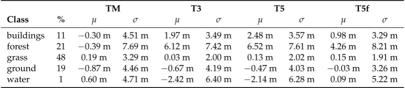
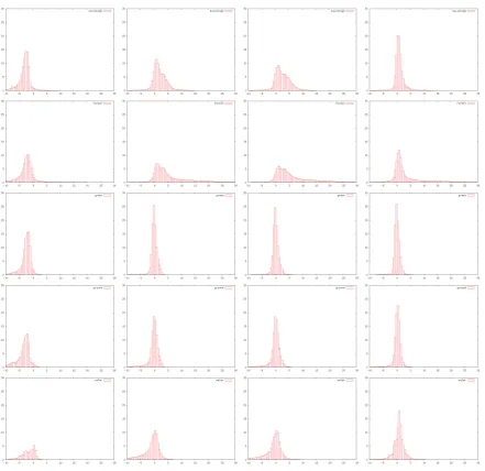
Using the classification shown in fig.4allows a more detailed evaluation of the derivations per class. Table1shows the classes, the coverage in percent of the class in the whole DTM and for each of the four derived test DTMs the mean shiftµand the standard deviationσ. Fig.10show the individual
distribution plots for each class.
Table 1.Classes used for detailled evaluation, coverage in percent of the class in the whole DTM, mean shiftµand standard deviationσfor DTMi−DTMre fper class.
TM T3 T5 T5f
Class % µ σ µ σ µ σ µ σ
buildings 11 −0.30 m 4.51 m 1.97 m 3.49 m 2.48 m 3.57 m 0.98 m 3.29 m forest 21 −0.39 m 7.69 m 6.12 m 7.42 m 6.52 m 7.61 m 4.26 m 8.21 m
grass 48 0.19 m 3.29 m 0.03 m 2.00 m 0.13 m 2.02 m 0.15 m 1.91 m
ground 19 −0.87 m 4.46 m −0.67 m 4.19 m −0.47 m 4.03 m −0.03 m 3.26 m water 1 0.60 m 4.71 m −2.42 m 6.40 m −2.14 m 6.28 m 0.09 m 5.22 m
Figure 10.Histograms of differences DTMi−DTMre f for classes (top to bottom) “buildings”, “forest”,
“grass”, “ground” and “water”, from left to right: DTM TM, T3, T5, T5f, binning to 0.5 m, percentage of values
3.5. Evaluation of nDEMs, tree- and building-masks
A main usage of a DTM is the derivation of off-ground objects or a nDEM. So in this evaluation we calculated the nDEMs for all derived DTMs and from them a tree- and a building-mask using a height-threshold of 3 m. Afterwards these masks were compared to the masks derived using the ground-truth DTM. For this the whole number of pixels of the reference height mask were calculated for vegetation (Nv) and non-vegetation (Nn) areas. Using the DTM under investigation for the derived
height maskHMi = (DSM−DTMi>3 m)the true positives (TP), false positives (FP) and the false
negatives (FN) were calculated as
TPi=
∑
(HMi∩HMre f) FPi =∑
(HMi∩HMre f) FNi =∑
(HMi∩HMre f) (1)Table2shows the results using the completeness asTPi/Nand the correctness as 1−(FPi+
Table 2. Completeness (how many pixels were “high” in both DTM and reference) and correctness (how many pixels were same “high” or “low” in both) for all derived DTMs
building-mask tree-mask
DTM completeness correctness completeness correctness
TM 92.66 % 67.50 % 91.81 % 72.00 %
T3 71.79 % 62.95 % 68.00 % 64.96 %
T5 65.65 % 58.15 % 64.25 % 61.71 %
T5f 85.91 % 81.04 % 78.58 % 75.72 %
As can be seen in tab.2the correctness increased from the simple T3, T5 over TM to T5f but the completeness decreases. The filtered version of the step algorithm delivers the nominally best results of all calculations using the DSM-to-DSM-step method. But in contrast to the classical method the completeness of detected above ground objects can not be reached by the new method.
4. Discussion
Fig.11shows a profile across an area in the old city center starting from the river Salzach, going south across the cupola of the Dom and crossing the hill with castle Hohensalzburg on it. The filled input DSM is shown in red, the reference DTM in green. All other profile lines are the derived DTMs TM, T3, T5 and T5f.
Figure 11.Profile 870 m starting from river Salzach across the Dom and the castle Hohensalzburg, red: filled DSM, green: reference DTM, blue: TM, purple: T3, cyan: T5, brown: T5f, units: ellipsoid height in [m] vs. position in profile line in px [0.3 m]
To sum up the results from sections3and4the results of the DSM-to-DTM-step approach give better results for build-up areas conserving steep natural hills in cities better than the traditional morphological approach.
5. Conclusions
The presented simplified DSM-to-DTM-step method for deriving DTMs from unfilled DSMs gives good results in urban areas conserving also hilly regions in builtup context. But overall the results compared to a ground truth DTM or to the also simple traditional morphological DTM extraction method shows no significant improvements in the resulting DTMs. As in most approaches for extracing DTMs from DSMs any method is not useful for all cases. So our final recommendation will be calculating the DTMs using different methods, classifying the terrain using terrain and spectral classification methods and finally fusing the results of the different DTM methods using different weights for each classified type of terrain. In the previous example the DSM-to-DTM-step method may be used in steep hills in urban areas whereas other methods will be better in rural areas.
Conflicts of Interest:“The authors declare no conflict of interest.”
1. Li, Z.; Zhu, Q.; Gold, C.Digital Terrain Modeling - Principles and Methodology; Routledge Chapman and Hall, 2004.
2. Weidner, U.; Förstner, W. Towards automatic building extraction from high resolution digital elevation models. ISPRS1995,50 (4), 38–49.
3. Arefi, H.; Reinartz, P. Building reconstruction from Worldview DEM using image information. SMPR2011, 2011.
4. Perko, R.; Raggam, H.; Gutjahr, K.; Schardt, M. Advanced DTM Generation from Very High Resolution Satellite Stereo Images. ISPRS Annals of the Photogrammetry, Remote Sensing and Spatial Information Sciences 2015,II-3/W4.
5. Meng, X.; Wang, L.; Silvan-Cardenas, J.L.; Currit, N. A multi-directional ground filtering algorithm for airborne LIDAR.ISPRS Journal of Photogrammetry and Remote Sensing2009,64, 117–124.