Hardness Estimation of LWE via Band Pruning
∗Yoshinori Aono Le Trieu Phong Lihua Wang†
October 27, 2015
Abstract
This paper, examining the hardness of the search LWE problem, is a refined continuation of previous works including (Lindner-Peikert 2011, Liu-Nguyen 2013, Aono et al. 2013) using lattice reduction and lattice vector enumeration. We adopt the attack to the LWE using discrete Gaussian distribution, and propose a new bounding method named band pruning in lattice enumeration. We update the security estimations for several parameter sets proposed in the literature. Finally, using the data gained in our experiments, we derive an explicit formula linking the LWE’s parameters with the bit security.
Keywords: Search LWE, hardness, lattice reduction, lattice enumeration
1
Introduction
1.1 Background
Fix numbersnandq. The learning with errors (LWE) problem [23] is roughly the problem to find a secret vectorx∈Znfrom a set of samples (ai ∈
Zn,bi ∈Z) where
hai,xi+ei =bi(modq) fori=1,2, . . .
whereai is randomly sampled from{0, . . . ,q−1}nandeiis sampled from a distribution over a set of small
integers of deviations. (The detailed definition is in Section 2.3)
The hardness of the learning with errors problem is a gold mine for cryptographers. It has been widely used to ensure the security of numerous cryptographic schemes. Therefore, giving concrete parameters for the hardness is a must in practice.
1.2 Our Contributions
This paper is an update of lattice vector enumeration based analyses [6, 18] for the LWE problem, and gives security analyses for several proposed parameter sets [6, 17, 18]. In details, our technical contributions are as follows:
(i)we update (refine) the cost estimation of lattice reduction part using recent records in SVP challenge [2]. Besides the time for lattice reduction, we need to predict the lengths of Gram-Schmidt basis vectors as sharp
∗
An abridged part of this paper was presented in [6] as the analytic contribution. This manuscript extends that part significantly.
†
as possible to predict the cost of lattice point search and consider the trade-offbetween two timings. We give our new estimation under both Lindner-Peikert model [17] and Chen-Nguyen [12] model with modified coefficients.
(ii) we develop a new pruning method, which we will refer as the band pruning, to speed up the lattice vector enumeration. Our theoretical analysis considersdiscreteGaussian error vectors while the previous attacks [17, 18] only consider continuous Gaussian ones1, allowing more rigid security analysis using small (e.g., deviation less than 8.0) Gaussian parameters.
(iii)we give a new method to estimate the lattice vector enumeration cost, which is derived from the volume of a bit complicatedn-dimensional object (see Seciton 4.) To approximate the volume, we use a method inspired from Gama-Nguyen-Regev [13] in the conference version [6] though it was omitted due to the space limit. After the conference version, we find a new method to approximate the volume without using a random source, which was a drawback of the original method. For the completeness of the information, we give both methods in Section 4.2 and A.
(iv)combining these new techniques together, we give security estimations for several parameters and suc-cess probabilities. By curve fitting on the data gained in our experiments, we derive an explicit formula to link between the bit security and LWE’s parameters (n,q,s) as follows:
bit−security= 7.18n−219
ln(q)−1.66 ln(s) −87 (1)
The left hand sidebit-securityis defined as follows:
bit−securityof LWE(n,q,s)=log2 attacking time in seconds attack success probability
!
+log2(9·106) (2)
Here, the constant log2(9·106) to convert time in seconds to bit-security is from the result ofRC5-72
benchmark published indistributed.net. It makes a record that a standard Intel CPU can check about 9·106keys in second in one thread.
1.3 Discussion on the Possibility of Optimizing Bounding Function
As the cases to estimate SVP and CVP, we simulate the cost and success probability psucc when we search an area defined by the bounding function. It is clear that the optimized bounding function that achieves min-imizing cost with keeping some probability, gives the hardness of cryptographies. Several fast computing methods to approximate the cost andpsucchave been developed when we assume the target point distributes uniformly in the searching area, and it allows us to optimize bounding function.
On the other hand, we assume the error vector distributes as a discrete Gaussian in this paper. This discreteness makes the estimation of probability very complicated and the problem of optimizing bounding function becomes a practically hard problem. Efficient generation of optimal function is an interesting future work.
1.4 Related Works
The LWE problem in dimension n can be theoretically reduced to lattice problems in dimension √n as in [10]. On the practical side, to give the concrete security parameters, several attacks are proposed which
1Quoting from [17, Section 6]: “... to allow for a Gaussian parameters≥8, so that the discrete GaussianD
are mainly classified to three types. Since the polynomial-time equivalence between the decision and search versions [23], many known attacks consider the search version while the securities of schemes are from the decision version. A survey on recent algorithms for solving LWE is in Albrecht et al. [5].
Lattice-Based attacks: Micciancio and Regev [20] gave a distinguishing attack using lattice reduction to a gadget lattice basis of which the first vector of a reduced basis corresponds to the error vector. In this line, Bai-Galbraith [8] and Lauter et al. [16] investigated the analysis.
Subsequently, Lindner-Peikert [17] regarded the problem to find the error vector as the bounded distance decoding (BDD) and analyzed a randomized version of the Babai’s nearest plane algorithm. Liu-Nguyen [18] also considered the problem as BDD and estimated the computational cost by lattice enumeration with linear pruning. These works assume the noises are from a continuous Gaussian distribution. The attack in Aono et al. [6] improved all these attacks by viewing the LWE problem as the closest vector problem (CVP) in which the difference between the target vector and lattice vectors has a discrete Gaussian distribution.
When the Gaussian error is continuous, it is the problem to recover the received signals in MIMO wireless connection. Several lattice based algorithms have been proposed [19, 26].
BKW attacks: Because the LWE problem is a natural extension of the learning with parity noises (LPN) problem, namely, LPN is LWE withq = 2, algorithms for LPN problem can be adopted for solving LWE problems. While Blum-Kalai-Wasserman [9] was originally proposed to solve the LPN problem, it was imported to the cryptographic area [3] and has been deeply investigated. The early attacks have a drawback that requires exponential number of samples, that does not match the real scheme, whereas the problem is avoided by considering trade-offbetween the complexity and number of samples.
Algebraic attacks: This type of LWE attacking algorithm is converting the original problem to an algebraic equation over integers. Arora-Ge [7] proposed a method to convert the problem to a large dimensional linear equation. The algorithm was further improved by the Gr¨oebner basis technique [4].
1.5 Roadmap
We give necessary lemmas and theorems, and introduce several previous works in Section 2. We fix the models and give our cost and probability estimation for the lattice reduction part in Section 3 and for the lattice enumeration part in Section 4. In Section 5, we propose a method to set our bounding function used in lattice enumeration, and give our new estimation for LWE problem and concrete formula.
2
Preliminaries
Throughout this paper, we use log2and ln to denote the logarithms of base 2 and of natural base.
2.1 Lattices
For a set of linearly independent vectors (v1, . . . , vm), which is called a lattice basis, the lattice is set L := nPm
i=1aivi:ai∈Z
o
. We denote its Gram-Schmidt basis by tildes: ˜v1, . . . ,v˜m. The lattice volume or determinantis det(L) := Qm
i=1||v˜i||. For a fixed lattice basis (v1, . . . , vm) and a vectorv =
Pm
i=1xiv˜i, itsk-th
2.2 Discrete Gaussian
For the derivation parameter s > 0, the discrete Gaussian distribution ψs overZ is the random variable
whose density function atyis
Pr[ψs=y]=
exp(−πy2/s2)
1+2P∞
j=1exp(−πj2/s2)
. (3)
Denote the denominator in (3) as W(s). The m-dimensional discrete Gaussiane = (e1, . . . ,em) ∈ ψms is
defined by taking eacheifromψsindependently. Thus, we have
Pr[ψm
s =(e1, . . . ,em)]=
exp(−π||e||2/s2)
W(s)m . (4)
To treat the discrete Gaussian, the following lemma is necessary.
Lemma 1 For given m,B∈Zand small s∈R, we can efficiently compute the probability
p(m,B) := Pr
e←ψm×1 s
h
||e||2= Bi=
X
y∈Zm
||y||2=B
exp(−π||y||2/s2)
W(s)m
with high accuracy.
Proof. Consider the sequence {p(1,i)}i=0,1,... that is easily computed with high accuracy. By the
rela-tion p(m+1,B) = PB
j=0p(m,j)· p(1,B− j),{p(m+1,i)}i=0,1,... is the convolution of {p(m,i)}i=0,1,... and
{p(1,i)}i=0,1,.... Considering an aborted sequence{p(1,i)}i=0,1,...,N−1 of length Nof some power of two, the
convolution can be efficiently computed by the FFT.2
In this paper, it is enough by computing these values in 512-bit precision because we will argue the parameters that achieve at most about 256-bit security. If one wants to obtain these values in very high accuracy, compute its numeratorη(B,m) exp(−πB/s2) whereη(B,m) is the number of integer solutions of the Diophantine equation x21+ · · ·+ xm2 = B. This is just the coefficient of xB of a special case of the Jacobi theta function (P∞
j=−∞xj 2
)m = (1+2P∞ j=1x
j2)m. The coefficients are easily derived by computing
this function modulox`for some`.
With the same method, the probability that||e||is within some range is also computable:
Pr
e←ψms×1
h
B1≤ ||e||2≤B2
i
= X
B∈[B1,B2]∩Z
Pr
e←ψms×1
h
||e||2= Bi.
2.3 The (Search) Learning With Errors Problem
The search LWE is defined as follows. For given ( A ∈ Zm×n, b = Ax+e ∈ Zm×1) where x ∈ ψn×αq1 and
e∈ψm×αq1, the problem is to find the secret vectorxor equivalently to finde. Let us denote as LWE(n, α,q). For given instance (A,b), the standard lattice based attack considers the lattice Λq(A) := {z ∈ Zm :
∃xsuch thatz = Ax(modq)} whose vectorzclosest to bderives the error vectore = b−z. Assume the latticeΛq(A) is given by rows of aq-ary matrix:
"
qIm−n 0
A0 In
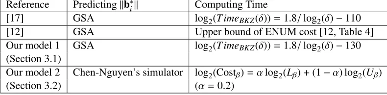
Reference Predicting||b∗i|| Computing Time
[17] GSA log2(T imeBKZ(δ))=1.8/log2(δ)−110
[12] GSA Upper bound of ENUM cost [12, Table 4]
Our model 1 GSA log2(T imeBKZ(δ))=1.8/log2(δ)−130
(Section 3.1)
Our model 2 Chen-Nguyen’s simulator log2(Costβ)=αlog2(Lβ)+(1−α) log2(Uβ)
(Section 3.2) (α=0.2)
Table 1: Summery of attacking models among previous works and this paper
whereA0 is uniquely determined under modulo qfrom the instance. We use (b1, . . . ,bm) and (˜b1, . . . ,b˜m)
to denote a reduced basis and its Gram-Schmidt basis. As we will introduced later, the cost of lattice enumeration part can be approximated using only the Gram-Schmidt lengths (||b∗1||, . . . ,||b∗m||) and bounding coefficients.
2.4 Experimenting Environment
We used the boost library [1] to compute the bounding functions in lattice vector enumeration, and to compute the attacking cost and success probability. The preliminary experiments in Section 3 was performed with usingntllibrary [27].
3
Models for Lattice Reduction
To analyse the lattice based attack for LWE, it needs to fix the model for lattice reduction part. Concretely, the lengths||b˜i||of Gram-Schmidt basis which is used to estimate the lattice vector enumeration part, and
time for lattice reduction. Following the previous works [17, 18], we consider two models, the geometric series assumption (GSA) model [24] and BKZ 2.0 model [12] with modifying constant factor using Lattice Challenge records [2]. Table 1 shows the summery, and below we give the details of them.
3.1 Geometric Series Assumption Model
Since the target lattice is q-ary, following Schnorr [24] and experiments in [17], we set the following as-sumption here.
Assumption 1 The graph ofln||ebi||consists of horizontal line||ebi||= q (if they exist), slope of0.5 lnr, and
line||ebi||=1.
Here,ris a constant in GSA that assumes||ebi||2/||b1||2=ri−1for a reduced basis. It connects to the root
Hermite factorδby the relationr =δ−4m/(m−1)if the Gram-Schmidt basis lengths consist only the slope part. The condition is explicitly given as follows.
1<||ebi||<qfor alli∈[m] ⇔ lnq− q
ln2q−4nlnδlnq
!
/2 lnδ <m< p(nlnq)/lnδ (5)
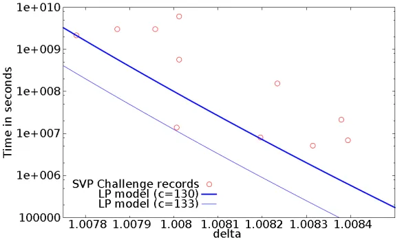
Computing time: In [17], they estimated the cost of BKZ algorithm to achieve the root Hermite factorδas
T imeLP(δ)=21.8/lg(δ)−c[single-core seconds],
where they usedc= 110. Figure 1 plots recent records in SVP Challenge. From the figure, we decided to usec=130 as the average performance of recent algorithms.
Figure 1: Relation between root Hermite factor and computing time published in SVP Challenge, and modified Lindner-Peikert estimation..
Drawback of this model: Clearly, there exists a lower bound ofδfrom the lengths of the shortest vector. We can see that substituting its value,T imeLP =2Θ(n/ln(n)). Thus, it derives a subexponential algorithm for SVP, which is probably hard to realize. For detailed argument, see Albrecht et al. [5].
Moreover, it is known that Schnorr’s GSA does not hold in general when the basis is very reduced [11]. Remark that Liu-Nguyen [18] also employed this model with modified computing time from Chen-Nguyen’s BKZ 2.0 simulator.
To avoid these drawbacks, we use the BKZ 2.0 Model.
3.2 BKZ 2.0 Model
To modify the drawback of GSA model., we use Chen-Nguyen’s estimation and simulator.
From [12, Table 4,5], we extrapolate the lower and upper bound of the number of processed nodes in one enumeration of BKZ-βas
log2(Uβ)=0.000784314β2+0.366078β−6.125, and log2(Lβ)=0.000409753β2+0.237652β−19.3668.
Since they have a significant gap, we need to select a good medium estimation to meet the experimental data. For this purpose, we assume the cost of enumeration satisfies
and for several fixed α ∈ [0,1] and lattice dimension, we execute their BKZ simulator to solve the SVP challenge problems and search the optimal βminimizing total enumeration cost. The simulation starts at the simulated LLL-reduced basis that satisfies GSA and δ = 1.022 whose constant is from [21]. Total enumeration cost in seconds is
TimeBKZ2.0(n, β, ]Tours)=]Tours·
n−1
X
i=1
Costmin(β,n−i+1)/(5.0·107)[sec] (7)
Comparing with the recent records (see Figure 2), we decide thatα = 0.2 gives the practical lower bound to the lattice reduction cost at state of the art, and we will use in this paper. Here, the constant 5.0·107is decided from our benchmark on lattice enumeration.
Figure 2: Costs for solving SVP Challenge problems simulated by Chen-Nguyen’s BKZ 2.0 simulator. Lower and upper bounds, costs whenα=0.2 and points from [2].
4
Model for Lattice Vector Enumeration
We introduce our model for searching error vector, success probability and computing cost adopting to the discrete Gaussian model.
Lattice vector enumeration algorithm: To find the error vector, our attack employs an exhaustive search algorithm [15] (and its modifications [18, 25]) with pruning technique adopted for discrete Gaussian LWE. Since the coordinates of error vector are from a Gaussian, we can bound its projected lengths from the lower and the upper.
The outline of algorithm is as follows: Consider a search tree whose root is labeled by the vectorb. For each node labeled byvat depthk, its children have labels of the formv−a·bm−kwitha∈Z. Thus, nodes at depthkare labeled by vectors of the formb−Pm
i=m−k+1ai·bi∈b−Λq(A) and the desired vectoreexists
at depthm. The algorithm is the depth-first search for this tree and a node is pruned if the projected length
Assumptions to set the bonding coefficients:
Assumption 2 [13, Heuristic 3] the distribution of matrix(˜b1/||b˜1||, . . . ,bm˜ /||bm˜ ||) of a random reduced
basis looks like a uniform distribution over Rm×mO in the meaning of Haar measure, the set of normalized orthogonal matrix of degree m. In particular, for a fixed pointw∈Sm−1,wV distributes uniformly over Sm−1 when V←Rm×mO .
Note that this assumption does not hold in general q-ary lattices, because for some reduced bases and parameters,ebi’s for small and large indexes remain as (0, . . . ,0,q,0, . . . ,0) and (0, . . . ,0,1,0, . . . ,0),
respec-tively. To avoid this phenomenon, we restricted the range ofmandδby (5) in parameter setting.
From now on, denotevi :=ebi/||ebi||. Forb = Ax+e, write the error vectore := b−z = (e1, . . . ,em) =
Pm
i=1αiebiwithz=Ax∈Λq(A). Byhe,ebii=αi||ebi||2, the projective length of each node is
πm−k+1
b−
m
X
i=m−k+1
ai·bi 2 = m X
i=m−k+1
α2
i||ebi||2=
m
X
i=m−k+1
he,ebi/||ebi||i2 =
m
X
i=m−k+1
he, vii2.
We discuss the distribution of this length when (v1, . . . , vm) ← Rm×mO ande ← ψm×s 1. LetV = (v1, . . . , vm).
hvi, vji = δi j and V−1 = VT hold. Since he, vii = hV−1e,V−1vii = (V−1e)i (the i-th element of
vec-tor) and ||V−1e|| = ||e||, the distribution of Pk
i=1he, vii2 is the same as that of ||e||(g21 + · · ·+ g2k) where
(g1, . . . , gm) $
←Sm−1. In other words, the norm distribution is unchanged, whereas its position distributes over the scaled (n−1)-sphere. We denote this distributionCs,m. This is our model of the distribution of error
vector.
4.1 Definitions of Cost and Probability
For fixed parameters and bounding functionsLi andRi, we define the success probability of the attack as follows.
Definition 1 Success probability of the attack.
PrhL2k < k
X
i=1
he, vii2<R2k ∀k∈[m]
i
. (8)
Here, the probability is over e←ψm×1
s and(v1, . . . , vm)←Rm×mO .
The above can be decomposed as
Pr
f←Cs,m
h
L2k < k
X
i=1
fi2<R2k ∀k∈[m]i=
R2 m
X
u=L2 m
Pr
f←Cs,m
h
k
X
i=1
fi2∈[Lk2,R2k]∀k∈[m]
||f||
2 =ui
× Pr
f←Cs,m
[||f||2=u].
Remark that the latter factor Prf←Cs,m[||f||
2 = u] is computable by using Claim 1, and we compute the
other part by the Monte-Carlo sampling over sphere.
Definition 2 Cost of lattice vector enumeration.
]ENU M= m
X
k=1
VolC(L1, . . . ,Lk;R1, . . . ,Rk)
Qm
i=m−k+1||ebi||
.
Here, C(L1, . . . ,Lk;R1, . . . ,Rk)is the object defined by
(x1, . . . ,xk)∈Rk:L2i < i
X
`=1
x2` <R2i for∀i∈[k]
.
To find a good cost estimation, we need to approximate the volume of this object.
4.2 Approximating Volume Factors
Fix an integerk ≥ 1. Let the sequences (L1, . . . ,Lk) and (R1, . . . ,Rk) are monotonic increasing and satisfy
0≤Li <Ri≤1 for alli. We can assumeRi ≤1 without loss of generality; if not, we normalize the sequence by dividingRk. For simplicity, we uselkandrk to denote the sequence respectively. Then denote the object
C(lk,rk) :=C(L1, . . . ,Lk;R1, . . . ,Rk).
To find a good approximation of VolC(lk,rk), in the conference version [6], we used the random sampling method inspired from Gama-Nguyen-Regev’s analysis for lattice vector enumeration [13]. Because this method requires the random source, the estimated volume is perturbated in each execution for the same parameters. It is a barrier to search optimized parameters correctly. Moreover, it requires a heavy computing when the dimension is high. To avoid the drawbacks, we develop a new approximating method. Although the old algorithm is not used in this paper, we give it in Appendix A for completeness of information because it was omitted in the conference proceeding.
Our method in theory: Since C(lk,rk) ⊂ [−1,1]k, the volume can be written by the probability Pk =
Prx←[−1,1]k[x∈C(lk,rk)] times 2k.
For a point x in an Euclidean space of dimension≥ j, we denote the eventEj be thatxsatisfies L2j <
Pj
`=1x 2
` <R2j. The desired probability is Prx∈[−1,1]k[E1· · ·Ek]. Fori=1, . . . ,k, we let Pi= Pr
x←[−1,1]i[Ei|E1· · ·Ei−1]
and we have by the chain rule
Pk = Pr
x←[−1,1]k[Ek|E1· · ·Ek−1]·x←[Pr−1,1]k[E1· · ·Ek−1]
= Pr
x←[−1,1]k[Ek|E1· · ·Ek−1]·x←[−Pr1,1]k−1[E1· · ·Ek−1]
= Pr
x←[−1,1]k[Ek|E1· · ·Ek−1]·Pk−1.
We compute the probability by induction starting with the base caseP1=R1−L1. By definition, the conditional probability is
αk := Pr
x←[−1,1]k[Ek|E1· · ·Ek−1]= x←C(lk−1,Prrk−1)×[−1,1]
DenoteFk−1(z) andGk(z) be the probability density function (p.d.f.) of|x|2and|y|2whenx $
←C(lk−1,rk−1)⊂
Rk−1 andy $
←C(lk−1,rk−1) ×[−1,1] ⊂ Rk, respectively. It is clear that the distribution of|y|2 is that of
|x|2+(x0)2wherexis the same as above andx0 ←[−1,1] independently. Thus, we have the relation
Gk(z)= Fk−1(z)∗H(z) :=
Z 1 0
Fk−1(y)H(z−y)dy. (10)
where
H(z)=
( 1/2√
z (0<z<1)
0 (otherwise)
is the p.d.f. ofx2whenx←$ [−1,1].
By the relationC(lk,rk) = C(lk−1,rk−1)×[−1,1]∩ {x ∈ Rk|L2k ≤ |x|
2 ≤ R2
k}, the probability (9) can be
computed by
Pr
x←C(lk−1,rk−1)×[−1,1]
[L2k ≤ |x|2 ≤R2k]=
Z R2k L2
k
Gk(z)dz. (11)
Also, we have the relation between the p.d.f.
Fk(z)=
(
(1/αk)Gk(z) (L2k ≤z≤R2k)
0 (otherwise) (12)
Therefore, the probability is
Pk = k
Y
i=1
αi.
Our method in practice: Our algorithm to compute the volume approximates the p.d.f. Fk(z) andGk(z)
within the range [0,1] by a real number sequence fj=(fj,0, . . . , fj,N−1) of lengthNwhere fj,`is an
approx-imation for
Z (`+0.5)/N
(`−0.5)/N
Fj(x)dx. (13)
The sequencesgj =(gj,0, . . . , gj,N−1) andh=(h0, . . . ,hN−1) are also used forGj(x) andH(x) in (13).
We simulate the theoretical argument as follows. For the base case, simulate
F1(x)=
(
2√(R1−L1)z (L21≤z≤R21)
0 (otherwise) andH(z).
To simulate the convolution (10) of functions, we use the convolution of sequences{fj∗gj}`={P`i=0 fj,igj,`−i}`
which can be efficiently computable by using FFT.
The integral at the right-hand side of (11) is simulated by a simple addition:
e
αk= `2
X
i=`1
gi
with`1=[L2k ·N] and`2=[R2k ·N]. The cut-off(12) is multiply-then-zeroing:
fk,` =
( g
k,`/αek (`=`1, . . . , `2)
0 (otherwise)
5
LWE Hardness Estimation
In the rest of this section, the notation Pr without indicating distribution means that the probability over
f ←Cs,m.
5.1 Our Bounding Function Setting
The goal of this section is to give a constructive proof of the following theorem.
Theorem 1 (Band pruning) For any probability parameter p ∈ [1/m,1), under our model, we can effi -ciently compute numbers Lkand Rkso that the success probability is larger than1−p.
Proof. We again denote the event Ek that satisfies L2k < Pki=1 fi2 < R
2
k and ¯Ek for its inverse. Then the
probability that the error vector is found is psucc:=Pr [E1· · ·Em].
From Lemma 1 it is possible to compute the lower and upper bounds of error vector lengthsLmandRm
so that
Pr
e←gZms
h
||e||2>R2mi≤ 1
2m and e Prg ←Zms
h
||e||2<L2mi≤ 1
2m.
Using these values, we have
psucc =Pr [Em]·Pr [E1· · ·Em−1|Em]≥ 1−
1
m
!
·Pr [E1· · ·Em−1|Em].
To bound the probability factor, we consider the individual probability Pr[Ek|Em]. For any Lk <Rk, we have
Pr[ ¯Ek|Em]= X
u∈[L2 m,R2m]∩Z
Prh
k
X
i=1
fi2≤ L2k
||f||
2=ui
Prh||f||2=ui+ X u∈[L2
m,R2m]∩Z
Prh
k
X
i=1
fi2 ≥R2k
||f||
2=ui
Prh||f||2=ui.
(14) Each conditional probability can be represented by the incomplete beta function. For instance, the case of lower bound is
Prh
k
X
i=1
fi2≤L2k
||f||
2=ui
= Pr
(h1,...,hm)←Sm
h
k
X
i=1
h2i ≤ L
2
k u
i
= IL2 k/u
k
2,
m−k
2
!
:=
Z Lk2/u
0
tk2−1(1−t) m−k
2 −1dt
B(k/2,(m−k)/2) ,
and the other case is similar. Here, foru≤ L2k, we regard the probability is one. The other factor Pr[||f||2=u] can be computed by Claim 1. Therefore, the tail probability (14) can be computed efficiently by summing up 2(R2m−L2m) terms.
We setL2k andR2k so that the both factors in the right-hand side of (14) arep0/2(m−1) where p0= mp−m−11. Thus, we have Pr[ ¯Ek|Em]= p0/(m−1) fork∈[m−1], and
Pr[E1· · ·Em−1|Em]>1+ m−1
X
k=1
Pr[Ek|Em]=1− p0. (15)
Practical relation betweenp0andpsucc: We remark on the success probability analysis. Since the
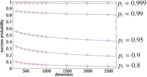
inequal-ity (15) uses a simple union bound, there exists a significant gap. To check it, we performed the preliminary experiment. Figure 2 shows the relation among dimension m, individual probability p0, and the success probabilitypsuccwhen setting bounding functionLk andRk so that Pr[Ek|Em]= p0when s=8. The circles
and curves indicate the experimental result using the above formula, and the result of curve fitting where we set
psucc= pY whereY =a+bmc+d pe.
and
(a,b,c,d,e)=(0.0345,3.32,0.2,7.93,35.8).
Using this relation, we can set pwhen the target probabilitypsuccis given. We will use this formula to setpfrom a targetpsucc ∈[0.01,0.99].
Figure 3: Relation betweenpandpsuccfor several dimensions (temporal)
5.2 LWE Parameters
We give our experimental results of LWE attacking cost.
Comparison to Previous Results under GSA: Table 2 gives the comparison among previous and our attacks for Lindner-Peikert’s parameters under GSA. We again remark that the GSA does not hold exactly and its estimation for timing of lattice vector enumeration small.
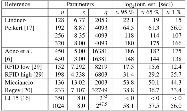
Updated parameters: Table 3 gives updated attacking costs in various success probabilities from several published papers.
For given parameter set (n,q,s), we consider the additional parameters (m, β, ]Tours), and simulate||ebi||
ofm-dimensionalq-ary lattices after]Tours tours of BKZ-βby using Chen-Nguyen’s simulator. Then, the total attacking cost is given by the sum of (7) and enumeration cost in Section 4:
Our Estimation(n,q,s)[sec]=TimeBKZ+]ENU M/(5·107) (16)
Lindner-Peikert [17] Liu-Nguyen [18] this workwith GSA (Our model 1)
Gaussian model Continuous Continuous Discrete
log2(tBKZ(δ)) 1.8/log2(δ)−110 [12]’s upper 1.8/log2(δ)−130 ]ENU M/sec./thread 215 107=223.25[12] 5·107=225
n s q log2(time in second in single thread)andsuccess probability
128 6.77 2053 32 ≈100% 23.6 ≈63.21% 11.5 ≈95.4%
192 8.87 4093 78 ≈100% 62.8 ≈63.21% 52.4 ≈95.7%
256 8.35 4093 132 ≈100% 105.5 ≈63.21% 95.8 ≈95.7%
320 8.00 4093 189 ≈100% – – 139.7 ≈95.6%
Table 2: Comparison among several attacks on LWE using single-thread time for Lindner-Peikert parame-ters.All models assume that||ebi||of reduced lattices satisfy the GSA.
Reference Parameters log2(our. est. [sec])
n s q ≈95 % ≈65 % ≈1 %
Lindner- 128 6.77 2053 22.1 19 15
Peikert [17] 192 8.87 4093 64.5 61.3 56.0
256 8.35 4093 118 114 107
320 8.00 4093 180 175 166
Aono et al. 450 5.00 16381 186 182 175
[6] 450 3.00 16381 148 144 138
RFID low [29] 152 7.292 8219 17.5 15.6 12.4
RFID high [29] 198 4.338 6803 31.4 29.2 25.7
Micciancio- 136 13.02 2003 53.8 50.1 44.3
Regev [20] 233 7.107 32749 38.8 36.7 33.4
LL15 [16] 350 8.0 252 <0 <0 <0
1024 8.0 247.5 58.1 57.5 56.0
We estimate Lindner-Peikert parameters by our attack usingpsucc≈10−8. The result is given in Table 4.
Be-cause the setting method of bounding functions are not investigated enough, the speed up is minor compared to the probability.
(n,q,s) ≈95% ≈10−8 (192,8.87,4093) 64.5 54.9 (256,8.35,4093) 118 101 (320,8.00,4093) 180 159
Table 4: Cost comparison between high and very low probabilities
Explicit formula for parameter setting: Since our prediction requires a heavy computation to obtain results, we give a formula of attacking time for parameter (n,s,q) by curve fitting. We assume the form of formula as
log2(T imeLW E [sec])=
Bn−C
lnq−Alns −D
which was derived from the estimation in [14]. Using the estimation in [17], they proposed a necessary LWE dimensionn ≥ log(q/s)·(k+110)/7.2 to achieve 2k attacking time/probability. Remark that the formula
of [14] is a theoretical estimation. In contrast, our formula is from real experiments. In addition, the models under the formulas are also different, so it is hard to directly compare them.
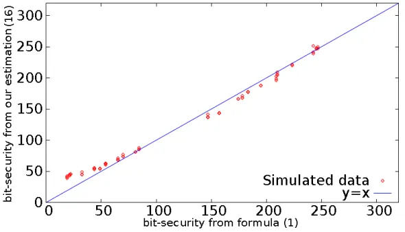
With our hardness estimations for several parameters satisfies n ∈ [100,1000], q ∈ [210,252], s ∈
[2.0,14.0] andpsucc ∈[0.01,0.95], besides Table 3, we fix the coefficients (A,B,C,D)=(1.66,7.18,219,110)
by the least square estimation. Figure 4 is the points whose coordinates are the security estimations by this formula and our method by (2). We can see the points are on the liney= xwhich means our formula works well.
Figure 4: Verifying our security estimation formula
Note that this estimation assumess>1.5 because if the deviation is too small, the lattice point
enumer-ation can be done significantly fast. We also assume p ≥ 0.01 because the estimated security (2) is much
smaller than that by the formula when the probability is small. For low probability situation, it needs to perform the individual simulations.
6
Conclusion
We update the lattice based attack for LWE problem and adopt the previous attack to the discrete Gaussian model. We also give an explicit formula tobit securityestimation. Using this result, we can set the concrete parameters having anybit securityin LWE based scheme.
References
[1] Boost C++Libraries,http://www.boost.org/.
[2] TU Darmstadt SVP Challenge. http://www.latticechallenge.org/svp-challenge/.
[3] M. R. Albrecht, C. Cid, J. Faug`ere, R. Fitzpatrick, and L. Perret. On the complexity of the BKW algorithm on LWE. Des. Codes Cryptography, 74(2):325–354, 2015.
[4] M. R. Albrecht, C. Cid, J.-C. Faugere, R. Fitzpatrick, and L. Perret. Algebraic algorithms for LWE problems. Cryptology ePrint Archive, Report 2014/1018, 2014. http://eprint.iacr.org/.
[5] M. R. Albrecht, R. Player, and S. Scott. On the concrete hardness of learning with errors. Cryptology ePrint Archive, Report 2015/046, 2015.http://eprint.iacr.org/.
[6] Y. Aono, X. Boyen, L. T. Phong, and L. Wang. Key-private proxy re-encryption under LWE. In G. Paul and S. Vaudenay, editors, INDOCRYPT, volume 8250 ofLecture Notes in Computer Science, pages 1–18. Springer, 2013.
[7] S. Arora and R. Ge. New algorithms for learning in presence of errors. In L. Aceto, M. Henzinger, and J. Sgall, editors,ICALP (1), volume 6755 ofLecture Notes in Computer Science, pages 403–415. Springer, 2011.
[8] S. Bai and S. D. Galbraith. Lattice decoding attacks on binary LWE. In ACISP 2014, LNCS 8544,, pages 322–337, 2014.
[9] A. Blum, A. Kalai, and H. Wasserman. Noise-tolerant learning, the parity problem, and the statistical query model. J. ACM, 50(4):506–519, July 2003.
[10] Z. Brakerski, A. Langlois, C. Peikert, O. Regev, and D. Stehl´e. Classical hardness of learning with errors. In D. Boneh, T. Roughgarden, and J. Feigenbaum, editors,STOC, pages 575–584. ACM, 2013.
[12] Y. Chen and P. Q. Nguyen. BKZ 2.0: Better lattice security estimates. In D. H. Lee and X. Wang, editors,ASIACRYPT 2011, volume 7073 ofLecture Notes in Computer Science, pages 1–20. Springer, 2011.
[13] N. Gama, P. Q. Nguyen, and O. Regev. Lattice enumeration using extreme pruning. In H. Gilbert, edi-tor,EUROCRYPT 2010, volume 6110 ofLecture Notes in Computer Science, pages 257–278. Springer, 2010.
[14] C. Gentry, S. Halevi, and N. P. Smart. Homomorphic evaluation of the AES circuit. InAdvances in Cryptology - CRYPTO 2012 - 32nd Annual Cryptology Conference, Santa Barbara, CA, USA, August 19-23, 2012. LNCS 7417, pages 850–867, 2012.
[15] R. Kannan. Improved algorithms for integer programming and related lattice problems. In D. S. Johnson, R. Fagin, M. L. Fredman, D. Harel, R. M. Karp, N. A. Lynch, C. H. Papadimitriou, R. L. Rivest, W. L. Ruzzo, and J. I. Seiferas, editors,STOC, pages 193–206. ACM, 1983.
[16] K. Laine and K. Lauterr. Key recovery for lwe in polynomial time. Cryptology ePrint Archive, Report 2015/176, 2015.http://eprint.iacr.org/.
[17] R. Lindner and C. Peikert. Better key sizes (and attacks) for LWE-based encryption. In A. Kiayias, editor,CT-RSA, volume 6558 ofLecture Notes in Computer Science, pages 319–339. Springer, 2011.
[18] M. Liu and P. Q. Nguyen. Solving BDD by enumeration: An update. In E. Dawson, editor,CT-RSA, volume 7779 ofLecture Notes in Computer Science, pages 293–309. Springer, 2013.
[19] S. Liu, C. Ling, and D. Stehl´e. Decoding by sampling: A randomized lattice algorithm for bounded distance decoding. IEEE Transactions on Information Theory, 57(9):5933–5945, 2011.
[20] D. Micciancio and O. Regev. Lattice-based cryptography. In Post-Quantum Cryptography, pages 147–191. Springer, 2009.
[21] P. Q. Nguyen and D. Stehl´e. LLL on the average. InAlgorithmic Number Theory, 7th International Symposium, ANTS-VII, Berlin, Germany, July 23-28, 2006, Proceedings, pages 238–256, 2006.
[22] P. Q. Nguyen and B. Valle. The LLL Algorithm: Survey and Applications. Springer Publishing Com-pany, Incorporated, 1st edition, 2009.
[23] O. Regev. On lattices, learning with errors, random linear codes, and cryptography. In H. N. Gabow and R. Fagin, editors,STOC, pages 84–93. ACM, 2005.
[24] C.-P. Schnorr. Lattice reduction by random sampling and birthday methods. In H. Alt and M. Habib, editors,STACS 2003, volume 2607 ofLecture Notes in Computer Science, pages 145–156. Springer, 2003.
[25] C. P. Schnorr and M. Euchner. Lattice basis reduction: Improved practical algorithms and solving subset sum problems. InMath. Programming, pages 181–191, 1993.
[26] B. Shim and I. Kang. Sphere decoding with a probabilistic tree pruning. IEEE Transactions on Signal Processing, 56(10-1):4867–4878, 2008.
[28] R. Smith. Efficient Monte-Carlo procedures for generating points uniformly distributed over bounded regions. Operations Res., 32:1296–1308, 1984.
[29] Y. Yao, J. Huang, S. Khanna, A. Shelat, B. H. Calhoun, J. Lach, and D. Evans. A sub-0.5V lattice-based public-key encryption scheme for RFID platforms in 130nm CMOS.
A
Random Sampling Method to Approximate the Volume of
C
(
l
k,
r
k)
in the
Conference Version [6]
We also define the covering object for an even integerk≥2 by
C0(lk,rk)=
(x1, . . . ,xk)∈Rk :L2i < i
X
`=1
x2` <R2i for∀eveni∈[k]
.
Clearly,C(lk,rk)⊂C0(lk,rk).
An algorithm for approximating VolC(lk;rk) by induction is given as follows. For the base casesk = 1
and 2, they can be computed by VolC(L1;R1)=2(R1−L1) and approximated by the standard Monte-Carlo
sampling method, respectively. For simplicity, let us denote the intervalIk =[−Rk,Rk].
For evenk≥2, suppose (an approximation of) VolC(lk;rk) is computed. Then by the relation in (k+
1)-dimensional space
C(rk+1,lk+1)⊂C(rk,lk)×[−Rk+1,Rk+1]⊂C0(rk,lk)×[−Rk+1,Rk+1],
the volume ink+1 dimension is computed by the relation
VolC(rk+1,lk+1)=VolC(rk,lk)·2Rk+1×Pr
h
x∈C(rk+1,lk+1)
x∈C(rk,lk)×Ik+1 i
.
where the probability is over x ← C0(rk,lk)× [−Rk+1,Rk+1]. Here, the above holds for any probability
distribution over x ← S such thatS ⊃ x ∈ C(rk,lk)×[−Rk+1,Rk+1]. Following [13], we decided to take
S = C0(rk,lk)×[−Rk+1,Rk+1] that gives a better balance between the easiness of sampling and probability
ratio Pr[x∈C(rk,lk)×[−Rk+1,Rk+1]]. As shown below, uniform sampling fromC0(rk,lk) is easy and hence
the probability is easily approximated.
Next, consider the (k+2)-dimensional object. By the relation
C(rk+2,lk+2)⊂C(rk,lk)×Ik+1×Ik+2⊂C0(rk,lk)×Ik+1×Ik+2,
we can also compute the volume by
VolC(rk+2,lk+2)=VolC(rk,lk)·4Rk+1Rk+2×Pr
h
x∈C(rk+2,lk+2)
x∈C(rk,lk)×Ik+1×Ik+2 i
where the probability is overx←C0(rk,lk)×Ik+1×Ik+2.
Uniform sampling from even-tube-intersections. To approximate the probability, we need to perform uniform sampling fromC0(rk,lk). This can be done by generating
(√u1cosθ1,
√
u1sinθ1,
√
u2cosθ2, . . . ,
√
where (θ1, . . . , θk/2) is uniform over [−π, π]k/2andu=(u1, . . . ,uk/2) is uniform from the polygon
P(rk,lk) :=
u∈Rk/2
L
2 2i <
i
X
`=1
u`<R22i, ui ∈[0,1]∀i∈
" k 2 #
by the hit-and-run algorithm [28] for sampling points uniformly from this object.
The correctness follows from [13]. Here we give a proof outline. Let us consider the standard (k
/2)-simplex
∆k/2 =
w∈Rk/2
wi ≥0 for∀i∈[k/2] and
k/2
X
`=1
w` ≤1
that containsC0(rk,lk), and let (y1, . . . , yk/2) be the uniform sampling from the simplex. Then, the extended
vector (y1, . . . , yk/2,y) where ¯¯ y = 1− y1 − · · · −yk/2 has the Dirichlet distribution Dir(1, . . . ,1) of order
k/2+1. On the other hand, for θ over uniform [−π, π], (cos2θ,sin2θ) has the distribution Dir(1/2,1/2).
Hence, the compound random distribution is a tuple inRk+2
(y1cos2θ1, y1sin2θ1, y2cos2θ2, . . . , yk/2cos2θk/2,y¯cos2θk/2+1,y¯cos2θk/2+1)
whereθi are uniformly sampled from [−π, π] independently, has the distribution Dir(1/2, . . . ,1/2). Thus,
by a straightforward computation of probability density function, the component-wise squared distribution
(√y1|cosθ1|,
√
y1|sinθ1|, . . . ,
√
yk/2
sinθk/2
, p ¯ y
sinθk/2+1 , p ¯ y
cosθk/2+1 )∈R
k+2
is the uniformly random over the part of (k+2)-dimensional unit sphere
(z1, . . . ,zk+2)∈Rk+2:zi≥0 for∀iand k+2
X
i=1
z2i =1)
.
Therefore, extracting firstkcoordinates and removing the absolute function, it can be shown that
(√y1cosθ1,
√
y1sinθ1, . . . ,
√
yk/2cosθk/2)∈Rk
is the uniform distribution in the unit ball.
Finally, considering rejection sampling, that is, restricting∆k/2toP(rk,lk) corresponds to restricting the
![Figure 2: Costs for solving SVP Challenge problems simulated by Chen-Nguyen’s BKZ 2.0 simulator.Lower and upper bounds, costs when α = 0.2 and points from [2].](https://thumb-us.123doks.com/thumbv2/123dok_us/7922501.1315461/7.612.154.450.242.438/figure-solving-challenge-problems-simulated-nguyen-simulator-points.webp)