Implementing Candidate Graded Encoding Schemes from
Ideal Lattices
Martin R. Albrecht1, Catalin Cocis2, Fabien Laguillaumie3, Adeline Langlois4
1
Information Security Group, Royal Holloway, University of London
2 Technical University of Cluj-Napoca 3
Universit´e Claude Bernard Lyon 1, LIP (U. Lyon, CNRS, ENS Lyon, INRIA, UCBL)
4
EPFL, Lausanne, Switzerland and CNRS/IRISA, Rennes, France
Abstract. Multilinear maps have become popular tools for designing cryptographic schemes since a first approximate realisation candidate was proposed by Garg, Gentry and Halevi (GGH). This construction was later improved by Langlois, Stehl´e and Steinfeld who pro-posed GGHLite which offers smaller parameter sizes. In this work, we provide the first implementation of such approximate multilinear maps based on ideal lattices. Implementing GGH-like schemes naively would not allow instantiating it for non-trivial parameter sizes. We hence propose a strategy which reduces parameter sizes further and several technical improvements to allow for an efficient implementation. In particular, since finding a prime ideal when generating instances is an expensive operation, we show how we can drop this requirement. We also propose algorithms and implementations for sampling from discrete Gaussians, for inverting in some Cyclotomic number fields and for computing norms of ideals in some Cyclotomic number rings. Due to our improvements we were able to compute a multilinear jigsaw puzzle forκ“52 (resp.κ“38) andλ“52 (resp.λ“80).
Keywords.algorithms, implementation, lattice-based cryptography, cryptographic multi-linear maps.
1
Introduction
Multilinear maps, starting with bilinear ones, are popular tools for designing cryptosystems. When pairings were introduced to cryptography [Jou04], many previously unreachable cryptographic primitives, such as identity-based encryption [BF03], became possible to construct. Maps of higher degree of linearity were conjectured to be hard to find – at least in the “realm of algebraic geometry” [BS03]. But in 2013, Garg, Gentry and Halevi [GGH13a] proposed a construction, relying on ideal lattices, of a so-called “graded encoding scheme” that approximates the concept of a cryptographic multilinear map.
As expected, graded encoding schemes quickly found many applications in cryptography. Already in [GGH13a] the authors showed how to generalise the 3-partite Diffie-Hellman key exchange first constructed with cryptographic bilinear maps [BS03] to N parties: the protocol allows N users to share a secret key with only one broadcast message each. Furthermore, a graded encoding scheme also allows constructing very efficient broadcast encryption [BS03,BWZ14]: a broadcaster can encrypt a message and send it to a group where only a part of it (decided by the broadcaster before encrypting) will be able to read it. Moreover, [GGH`13b] introduced indistinguishability
obfuscation (iO) and functional encryption based on a variant of multilinear maps — multilinear jigsaw puzzles — and some additional assumptions.
encoding gives a level-pi`jqencoding. Additionally, a zero-testing parameterpzt allows testing
if a level-κelement is an encoding of 0, and hence also allows testing if two level-κencodings are encoding the same elements. Finally, the extraction procedure usespztto extract`bits which are
a “canonical” representation of a ring element given its level-κencoding. More precisely, in GGH we are given R“ZrXs {pXn
`1q, wherenis a power of 2, a secret elementzuniformly sampled inRq“R{qR(for a certain prime numberq), and a public elementy
which is a level-1 encoding of 1 of the formra{zsq for some smallain the coset 1`I. We are also
givenmlevel-iencodings of 0 namedxjpiq, for all 1ďiďκ, and a zero-testing parameterpzt. To
encode an element ofR{I at level-i(foriďκ), we multiply it byyi inRq (which give an element
of the form “c{zi‰q, where c is an arbitrary small coset representative). Then, we add a linear
combination of encodings of 0 at level-iof the formř
jρjx
piq
j to it where theρj are sampled from a
certain discrete Gaussian. This last step is the re-randomisation process and ought to ensure that the analogue of the discrete logarithm problem is hard: going from level-ito level-0, for example by multiplying the encoding byy´i. We will see later that the encodings of zero made public for
this step are a problem for the security of the scheme.
The asymmetric variant of this scheme replaces levels by “groups” which are identified with subsets oft1, . . . , κu. Addition of two elements in the same group stays within the group, multiplying two elements of different groups with disjoint index sets produces an element in the group defined by the union of their index sets. These groups are realised by defining onezifor each index 1ďiďκ
and then dividing by the appropriate product ofzi. Given a group characterised bySĎ t1, . . . , κu
we call the cardinality ofS its level.
We can distinguish between GGH instances where encodings of zero are made publicly available to allow anyone to encode elements and those where this is not the case. The latter are also called “Multilinear Jigsaw Puzzles” and were introduced in [GGH`13b] as a building block for
indistinguishability obfuscation. Such instances can be thought of as secret-key graded encoding schemes. To distinguish the two cases, we denote those instances where no encodings of zeroxpjiq are published as GGHs. In such instances the secret elements g and zi are required to encode
elements at levels above zero.
Security. Already in [GGH13a] it was shown that an attacker can recover the ideal pgqand the coset ofpgqfor any encoding at levelďκif encodings of zero are made available. However, since these representatives of eitherpgq or the cosets are not small, it was believed that these “weak discrete log” attacks would not undermine the central security goal of GGH – the analogue of the BDDH assumption. However, in [HJ15] it was shown that these attacks can be extended to recover short representatives of the cosets. As a consequence, if encodings of zero are published, then [HJ15] breaks the GGH security goals in many scenarios and it is not clear, at present, if and how GGH-like graded encoding schemes can be defended against such attacks. A candidate proposal to prevent weak discrete logarithm attacks was proposed in [CLT15, Appendix G], where the strategy is to change zero testing to make it non-linear in the encodings such that the attack does not work anymore. However, no security analyses was provided in [CLT15] and revision
20150516:083005of [CLT15] drops any mention of this candidate fix. Hence, the status of
GGH-like schemes where encodings of zero are published is currently unclear. However, we note that GGHs, where no encodings of zero are made available, does not appear to be vulnerable to weak
discrete log attacks if the freedom of an attacker to produce encodings of zero at the higher levels is also severely restricted to prevent generalisations of “zeroizing” attacks such as [CGH`15].
Such variants are the central building block of indistinguishability obfuscation, i.e. this case has important applications despite being more limited in functionality. Indeed, at present no known attack threatens the security of indistinguishability obfuscation constructed from graded encoding schemes such as GGH.
was later generalised in [CGH`15] and a candidate defence against these attacks was proposed
in [CLT15]. The authors of [CLT15] also provided a C++ implementation of a heuristic variant of this scheme. They report that theSetupphase of an 7-partite Diffie-Hellman key exchange takes 4528s (parallelised on 16 cores), publishing a share (Publish) takes 7.8s per party (single core) and the final key derivation (KeyGen) takes 23.9s per party (single core) for a level of securityλ“80.
Instantiation. The implementation reported in [CLT15] is to date the only implementation of a candidate graded encoding scheme. This is partly because instantiating the original GGH con-struction is too costly in practice for anything but toy instances. In 2014, Langlois, Stehl´e and Steinfeld [LSS14a] proposed a variant of GGH called GGHLite, improving the re-randomisation process of the original scheme. It reduces the numberm of re-randomisers, public encodings of zero, needed from Ωpnlognqto 2 and also the size of the parameter σ‹
i of the Gaussian used to
sample multipliersρj during the re-randomisation phase fromOrp2λλ n4.5κqtoOrpn5.5
?
κq. These improvements allow reducing the size of the public parameters and improving the overall efficiency of the scheme. But even though [LSS14a] made a step forward towards efficiency and in some cases no public re-randomisation is required at all (GGHs), GGH-like schemes are still far from being
practical.
Our contribution. Our main contribution is a first and efficient implementation of improved GGH-like schemes which we make publicly available under an open-source license. This implementation covers symmetric and asymmetric flavours and we allow encodings of zero to be published or not. However, since the security of GGH-like constructions is unclear when encodings of zero are published, we do not discuss this variant in this paper. We note, however, that our implementation provides a good basis for implementing any future fixes and improvements for GGH-based graded encoding schemes.
Implementing GGH-like schemes efficiently such that non-trivial levels of multilinearity and security can be achieved is not straight forward and to obtain an implementation we had to address several issues. In particular, we contribute the following improvements to make GGH-like multilinear maps instantiable:
‚ We show that we do not require pgqto be a prime ideal for the existing proofs to go through. Indeed, sampling an element gPZrXs {pXn
`1qsuch that the ideal it generates is prime, as required by GGH and GGHLite, is a prohibitively expensive operation. Avoiding this check is then a key step to allow us to go beyond toy instances.
‚ We give a strategy to choose practical parameters for the scheme and extend the analysis of [LSS14a] to ensure the correctness of all the procedures of the scheme. Our refined analysis reduces thebitsize ofqby a factor of about 4, which in turn reduces the required dimension n.
‚ We apply the analyses from [CS97] to pick parameters to defend against lattice attacks.
‚ For all steps during the instance generation we provide implementations and algorithms which work in quasi-linear time and efficiently in practice. In particular, we provide algorithms and implementations for inverting in some Cyclotomic number fields, for computing norms of ideals in some Cyclotomic number rings, for producing short representatives of elements modulopgq
and for sampling from discrete Gaussians inOrpnq. For the latter we use Ducas and Nguyen’s strategy [Duc13] Our implementation of these operations might be of independent interest (cf. [LP15] for recent work on efficient sampling from a discrete Gaussian distribution), which
is why they are available as a separate module in our code.
‚ We discuss our implementation and report on experimental results.
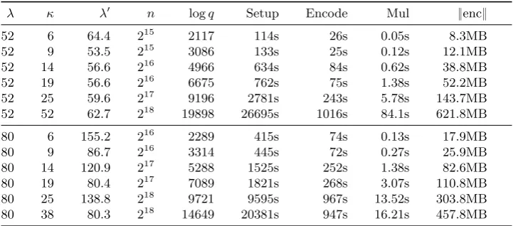
Our results (cf. Table 1) are promising, as we manage to compute up to multilinearity level κ“52 (resp. κ“38) at security levelκ“52 (resp.λ“80) in the asymmetric GGHs case. We note that much smaller levels of multilinearity have been used to realise non-trivial functionality in the literature. For example, [BLR`15] reports on comparisons between 16-bit encrypted values
λ κ λ1 n logq Setup Encode Mul
}enc}
52 6 64.4 215 2117 114s 26s 0.05s 8.3MB
52 9 53.5 215 3086 133s 25s 0.12s 12.1MB
52 14 56.6 216 4966 634s 84s 0.62s 38.8MB
52 19 56.6 216 6675 762s 75s 1.38s 52.2MB
52 25 59.6 217 9196 2781s 243s 5.78s 143.7MB 52 52 62.7 218 19898 26695s 1016s 84.1s 621.8MB
80 6 155.2 216 2289 415s 74s 0.13s 17.9MB
80 9 86.7 216 3314 445s 72s 0.27s 25.9MB
80 14 120.9 217 5288 1525s 252s 1.38s 82.6MB
80 19 80.4 217 7089 1821s 268s 3.07s 110.8MB 80 25 138.8 218 9721 9595s 967s 13.52s 303.8MB
80 38 80.3 218 14649 20381s 947s 16.21s 457.8MB
Table 1.Computing aκ-level asymmetric multilinear maps with our implementation without encodings of zero. Columnλgives the minimum security level we accepted, columnλ1 gives the actually expected security level based on the best known attacks for the given parameter sizes. Timings produced on Intel Xeon CPU E5–2667 v2 3.30GHz with 256GB of RAM, parallelised on 16 cores, but not all operations took full advantage of all cores. Setup gives the time for generating the GGH instance. Encode lists the time it takes to reduce an elementPZpwithp“NpIqto a small element inZrXs { pXn
`1qmodulopgq. Mult lists the time to multiplyκelements. All times are wall times.
Technical overview. Our implementation relies on FLINT [HJP14]. However, we provide our own specialised implementations for operations in the ring of integers of Cyclotomic number fields where the degree is a power of two and related rings as listed above.
Our variant of GGH foregoes checking if g generates a prime ideal. During instance genera-tion [GGH13a,LSS14a] specify to sampleg such thatpgqis a prime ideal. This condition is needed in [GGH13a,LSS14a] to ensure that no non-zero encoding passes the zero-testing test and to argue that the non-interactive N-partite key exchange produces a shared key with sufficient entropy. We show that for both arguments we can drop the requirement that g generates a prime ideal. This was already mentioned as a potential improvement in [Gar13, Section 6.3] but not shown there. As rejection sampling until a prime idealpgqis found is prohibitively expensive due to the low density of prime ideals inZrXs {pXn`1q, this allows speeding-up instance generation such that non-trivial instances are possible. We also provide fast algorithms and implementations for checking ifpgq ĂZrXs {pXn
`1qis prime for applications which still require primepgq.
We also improve the size of the two parametersqand`compared to [LSS14a]. We first perform a finer analysis than [LSS14a], which allows us to reduce thesize of the parameterqby a factor 2. Then, we introduce a new parameterξ, which controls what fraction ofqis considered “small”, i.e. passes the zero-testing test, which reduces the size ofq further. This also reduces the number of bits extracted from each coefficient `. Indeed, instead of setting `“1{4 logq´λwhereλis the security parameter, we set`“ξlogq´λwith 0ăξď1{4. We then show that for a good choice ofξ this is enough to ensure the correctness of the extraction procedure and the security of the scheme. Overall, our refined analysis allows us to reduce the size ofq« p3n32σ1‹σ1q
8κ
in [LSS14a] to q« p3n32σ1‹σ1q
p2`εqκ
which, in turn, allows reducing the dimension n. When no encodings of zero are published we simply setσ‹
1“1 and apply the same analysis.
would mean a significant step forward. Finally, establishing better estimates for lattice reduction and tuning the parameter choices of our schemes are areas of future work.
Roadmap. We give some preliminaries in Section 2. In Section 3 we describe the GGH-like asymmetric graded encoding schemes and the multilinear jigsaw puzzles used for iO. In Section 4, we explain our modifications to GGH-like schemes, especially concerning the parameter q. We also recall a lattice attack to derive the parameternand show that we do not require pgqto be prime. In Section 5, we give the details of our implementation.
2
Preliminaries
Lattices and ideal lattices. Anm-dimensional latticeLis an additive subgroup of Rm. A latticeL can be described by its basisB“ tb1, b2, . . . , bku, withbiPRm, consisting inklinearly independent vectors, for somekďm, called therank of the lattice. Ifk“m, we say that the lattice has full-rank. The lattice L spanned by B is given by L “ třki“1ci ¨bi, ci P Zu. The volume of the latticeL, denoted by volpLq, is the volume of the parallelepiped defined by its basis vectors. We have volpLq “adetpBTBq, where B is any basis ofL.
For n a power of two, let fpXq P ZrXs be a monic polynomial of degree n (in our case, fpXq “Xn
`1). Then, the polynomial ringR“ZrXs {fpXqis isomorphic to the integer latticeZn,
i.e. we can identify an elementupXq “řin“´01ui¨XiPR with its corresponding coefficient vector pu0, u1, . . . , un´1q. We also defineRq “R{qR“ZqrXs{pXn`1q(isomorphic to Znq) for a large
primeq andK“QrXs {pXn`1q(isomorphic toQn).
Given an element g P R, we denote by I the principal ideal in R generated by g: pgq “ tg¨u:uPRu. The idealpgqis also called anideal lattice and can be represented by itsZ-basis
pg, X¨g, . . . , Xn´1
¨gq. We denote byNpgqits norm. For anyyPR, letrysg be the reduction ofy moduloI. That is,rysg is the unique element inRsuch thaty´ rysgP pgqandrysg“řni“´01yiXig,
with yi P r´1{2,1{2q,@i,0 ď i ď n´1. Following [LSS14a] we abuse notation and let σnpbq
denotes the last singular value of the matrix rotpbq PZnˆn, for anybPI. ForzPR, we denote by MSB`P t0,1u`¨n the`most significant bits of each of thencoefficients ofzin R.
Gaussian distributions. For a vectorcPRnand a positive parameterσPR, we define the Gaussian distribution of centre c and width parameter σ as ρσ,cpxq “ expp´π||x´σ2c||2q, for allx P R
n.
This notion can be extended to ellipsoid Gaussian distribution by replacing the parameter σ with the square root of the covariance matrix Σ “ BBt
P Rnˆn with detpBq ‰ 0. We define it by ρ?
Σ,cpxq “ expp´π¨ px´cq t
pBtB
q´1px´cqq, for all x P Rn. For L a subset of Zn, let ρσ,cpLq “řxPLρσ,cpxq. Then, thediscrete Gaussian distribution overLwith centrecand standard deviationσ (resp. ?Σ) is defined asDL,σ,cpyq “ ρσ,cpyq
ρσ,cpLq, for ally PL. We use the notations ρσ
(resp.ρ?
Σ) andDL,σ (resp.DL,?Σ) whencis 0.
Finally, for a fixed Y “ py1, y2q PR2, we define:ErY,s “y1DR,s`y2DR,s as the distribution induced by sampling u “ pu1, u2q P R2 from a discrete spherical Gaussian with parameter s,
and outputting y “ y1u1`y2u2. It is shown in [LSS14a, Th. 5.1] that if Y ¨R2 “ I and s ě
maxp}g´1y
1}8,}g´1y2}8q¨n¨
a
2 logp2np1`1{εqq{πforεP p0,1{2q, this distribution is statistically close to the Gaussian distributionDI,sYT.
3
GGH-like Asymmetric Graded Encoding Scheme
We now recall the definitions given in [GGH`13b, Section 2.2] for the notions of Jigsaw specifier,
Multilinear Form and Multilinear Jigsaw puzzle.
Definition 1 ([GGH`13b, Def. 5]). AJigsaw specifieris a tuple pκ, `, Aqwhereκ, `P
Z` are parameters and Ais a probabilistic circuit with the following behavior: On input a prime number q,Aoutputs the primeq and an ordered set of`pairs pS1, a1q, . . . ,pS`, a`qwhere each aiPZq and
Definition 2 ([GGH`13b, Def. 6 and 7]). A Multilinear Form is a tuple F “ pκ, `, Π, Fq
whereκ, `PZ`are parameters andΠ is a circuit with`input wires, made out of binary and unary gates. F is an assignment of an index setI Ď rκs to every wire ofΠ. A multilinear form must satisfies constraints given in the original definition (on gates, and the output wire is assigned to
rκs).
We say that a Multilinear FormF“ pκ1, `1, Π, Fqis compatible withX“ ppS
1, a1q, . . . ,pS`, a`qq
ifκ“κ1,`“`1 and the input wires ofΠ are assigned to the sets S
1, . . . , S`. The evaluation ofF
onX is then doing arithmetic operations on the inputs depending on the gates. We say that the evaluation succeeds if the final output isprκs,0q.
We now define the Multilinear Jigsaw Puzzles.
Jigsaw Generator: JGenpλ, κ, `, Aq Ñ pq, X,puzzleq. This algorithm takes as inputλ, and a Jig-saw specifier pκ, `, Aq. It outputs a prime q, a private outputX and a public outputpuzzle. The generator is using a pair of PPT algorithmsJGen“ pInstGen,Encodeq.
InstGenpλ, κq Ñ pq,params, sq. This algorithm takesλandκas inputs and outputspq,params, sq, whereqis a prime of size at least 2λ,paramsis a description of public parameters, ands is a secret state to pass to the encoding algorithm.
Encodepq,params, s,pS, aqq Ñ pS, uq. The encoding algorithm takes as inputs the primeq, the parameters params, the secret state s, and a pair pS, aq with S Ď rκs and a P Zq and
outputsu, an encoding ofarelative toS.
More precisely, the algorithm runs the Jigsaw specifier on inputqto get`pairspS1, a1q, . . . ,pS`, a`q.
Then encodes all the plaintext elements by using theEncodealgorithm on eachpSi, aiqwhich
returnpSi, uiq. We have:
X “ pq,pS1, a1q, . . . ,pS`, a`qqandpuzzle“ pparams,pS1, u1q, . . . ,pS`, u`qq.
Jigsaw Verifier:JVerppuzzle,Fq Ñ t0,1u. This algorithm takes as input the public output of a Jigsaw Generatorpuzzle, and a multilinear formF. It outputs either acceptp1qor rejectp0q.
Correctness. For an outputpq, X,puzzleqand a formFcompatible withX, we say that the verifier JVeris correct if either the evaluation ofFonX succeeds andJVerppuzzle,Fq “1 or the evaluation fails and JVerppuzzle,Fq “ 0. We require that with high probability over the randomness of the generator, the verifier will be correct on all forms.
Security. The hardness assumptions for the Multilinear Jigsaw puzzle requires that for two different polynomial-size families of Jigsaw Specifiertpκλ, `λ, AλquλPZ` and tpκλ, `λ, A
1
λquλPZ` the public
output of the Jigsaw Generator onpκλ, `λ, Aλqwill be computationally indistinguishable from the
public output of the Jigsaw Generator onpκλ, `λ, A1λq.
3.1 Using GGH to construct Jigsaw puzzles
In Figure 1, we describe a GGH-like asymmetric graded encoding scheme without encodings of zero based on the definition of GGHLite from [LSS14a]. Below, we explain how to use those procedures to construct the Jigsaw Generator, described in [GGH`13b, Appendix A].
Jigsaw Generator. The Jigsaw Generator usesInstGen to generate all the public (params and pzt) and secret parameters of the multilinear map. Each level of the multilinear map will be
associated with a subset of the set rκs. To create the puzzle pieces, which are encodings of some elements ofR at different level, the Generator simply encodes some random elements at levelS Ă r1, κs, those are given aspuzzle.
Jigsaw Verifier. The verifier is given the public parameters params and pzt, a valid form Π
(which is defined [GGH`13b, Def. 6] in as a circuit made of binary and unary gates) andpuzzle,
‚ Instance generation. InstGenp1λ,1κq: Given security parameterλand multilinearity parameterκ, determine scheme parametersn,q,σ,σ1,`
g´1,`b,`as in [LSS14a]. Then proceed as follows:
‚ SamplegÐâDR,σ until}g´1} ď`g´1 andI“ pgqis a prime ideal. Define encoding domainRg “
R{ pgq.
‚ SampleziÐâUpRqqfor all 0ăiďκ. ‚ SamplehÐâDR,?
q and define the zero-testing parameterpzt“
”
h g
śκ i“1zi
ı
q. ‚ Return public parametersparams“ pn, q, `qandpzt.
‚ Encode at level-0 Enc0pparams, g, eq: Compute a small representative e1 “ res
g and sample an elemente2ÐâDe
1`I,σ1. Outpute2.
‚ Encode in group tiu.Encpparams, zi, eq: Given parametersparams,zi, and a level-0 encodingePR, outputre{zisq.
‚ Adding encodings. Addpparams, u1, u2q: Given encodings u1 “ “
c1{`śiPSzi ˘‰
q and u2 “
“
c2{`śiPSzi ˘‰
q withSĎ t1, . . . , κu:
‚ Returnu“ ru1`u2sq, an encoding ofrc1`c2sq in the groupS.
‚ Multiplying encodings.Multpparams, u1, u2q: Let S1 Ă rκs,S2 Ă rκswithS1XS2 “ H, given an
encodingu1“ ”
c1{ ´
ś
iPS1zi
¯ı
q
and an encodingu2“ ”
c2{ ´
ś
iPS2zi
¯ı
q : ‚ Returnu“ ru1¨u2sq, an encoding ofrc1¨c2sqinS1YS2.
‚ Zero testing at level κ.isZeropparams, pzt, uq: Given parametersparams, a zero-testing parameter pzt, and an encodingu““c{`śκi“´01zi˘‰q in the grouprκs, return 1 if}rpztusq}8ăq3{4and 0 else.
Fig. 1.GGH-like asymmetric graded encoding scheme adapted from [LSS14a].
4
Modifications to and parameters for GGH-like schemes
In this section, we first show that we do not require a prime pgq and then describe a method which allows to reduce the size of two parameters: the modulusq and the number`of extracted bits. In Section 4.3 then we describe the lattice-attack against the scheme which we use to pick the dimension n. Finally, we describe our strategy to choose parameters that satisfy all these constraints.
4.1 Non-prime pgq
Both GGHLite and GGH-like jigsaw puzzles as specified in Figure 1 require to sample ag such thatpgqis a prime ideal. However, finding such ag is prohibitively expensive. While checking each individualgwhetherpgqis a prime ideal is asymptotically not slower than polynomial multiplication, finding such a g requires to run this check often. The probability that an element generates a prime ideal is assumed to be roughly 1{pncqfor some constantcą1 [Gar13, Conjecture 5.18], so we expect to run this checknctimes. Hence, the overall complexity is at least quadratic innwhich is too expensive for anything but toy instances.
Primality ofpgqis used in two proofs. Firstly, to ensure that after multiplyingκ`1 elements inRg the product contains enough entropy. This is used to argue entropy of theN-partite
non-interactive key exchange. Secondly, to prove thatc¨h{g is big if c, hRg (cf. Lemma 2). Below, we show that we can relax the conditions on gfor these two arguments to still go through, which then allows us to drop the condition thatpgqshould be prime. We note, though, that some other applications might still requireg to be prime and that future attacks might find a way to exploit non-primepgq.
Entropy of the product. The next lemma shows that excluding prime factorsď2N and guaranteeing Npgq ě 2n is sufficient to ensure 2λ bits of entropy in a product ofκ`1 elements inRg with
Lemma 1. Let κ ě 2, λ be the security parameter and g P ZrXs {pXn
`1q with norm p “
Npgq ě 2n such that p has no prime factors
ď 2κ`2, and such that n ě κ¨λ¨logpλq. Then, with overwhelming probability, the product ofκ`1 uniformly random elements inRg has at least
κ¨λ¨logpλq{4 bits of entropy.
Proof. Writep“śri“1pei
i wherepi are distinct primes andeiě1 for alli. Let us consider the set
S“ tiP t1, . . . , ru:ei“1u. Then, following [CDKD14] we define ps“
ś
iPSpi as the square-free
part ofp. Asymptotically, it holds that #tpďx:p{psąpsuiscx3{4for some computable constant
c(cf. [CDKD14]). Since in our case we havexě2n, this implies that with overwhelming probability
it holds thatpsě ?
pand hence logppsq ěn{2.
By the Chinese Remainder Theorem, Rg is isomorphic to F1ˆ ¨ ¨ ¨ ˆFr where each “slot”
Fi “Zpeii . The set ofFi, foriPS corresponds to the square-free part of p. Those Fi are fields,
and each of them has orderpiě2N which means that a random element in suchFiis zero with
probability 1{pi. In those slots, the product ofN elements hasEs bits of entropy, where
Es“
ÿ
iPS
ˆ 1´N
pi
˙ logppiq.
First, aspiě2N for alliPS, the quotientN{piď1{2 and then
´ 1´Np
i
¯
ě1{2 for alliPS. This
implies that
Esě1{2
ÿ
iPS
logppiq “1{2 log´ ź
iPS
pi
¯
“1{2 logppsq.
Because logppsq ěn{2, we conclude that Esě n4 ě κ¨λ¨log4 pλq. [\
Probability of false positive. It remains to be shown that we can ensure that there are no false positives even ifpgqis not prime. In [GGH13a, Lemma 3] false positives are ruled out as follows. Letu“ rc{zκsq wherecis a short element in some coset ofI, and letw“ rpzt¨usq, then we have
w“ rc¨h{gsq. The first step in [GGH13a] is to suppose that}g¨w} and}c¨h} are each at most q{2, then, sinceg¨w “c¨hmodq we have that g¨w“c¨hexactly. We also have an equality of ideals:pgq ¨ pwq “ pcq ¨ phq, and then several cases are possible. Ifpgqis prime as in [GGH13a, Lemma 3], thenpgqdivides eitherpcqorphqand eithercor his in pgq. As, by construction, none of them is inpgqifcis not inI, either}g¨w}or}c¨h}is more thanq{2. Using this, they conclude that there is no smallc (not inI) such thatwis small enough to be accepted by the zero-test.
Our approach is to simply notice that all we require is thatpgqandphqare co-prime. Checking if
pgqandphqare co-prime can be done by checking gcdpNpgq,Nphqq “1. However, computingNphq
is rather costly becausehis sampled fromDZn,?q and hence has a large norm. To deal with this
issue we notice that if gcdpNpgq,Nphqq ‰1 then we also have gcdpNpgq,Nphmodgqq ‰1 which can be verified with a simple calculation. Now, interpreting hmodg as “a small representative ofhmodulo g”, we can computehmodg as h´g¨tg´1
¨hs, which produces an element of size
«?n¨ }g}. We can use this observation to reduce the complexity of checking ifpgqand phqare co-prime to computing two norms for elements of size }g} and «?n¨ }g} and taking their gcd. Furthermore, this condition holds with high probability, i.e. we only have to perform this testOp1q
times. Indeed, by ruling out likely common prime factors first, we expect to run this test exactly once. Hence, checking co-primality ofpgqand phq is much cheaper than finding a prime pgqbut still rules out false positives.
Finally, we note that recent proposals of indistinguishability obfuscation from multilinear maps [Zim15,AB15] requires composite order maps. These are not the maps we are concerned with here as in [Zim15,AB15] it is assumed that the factorisation ofpgqis known. However, we note that our techniques and implementation easily extend to this case by consideringg“g1¨g2 for
known co-primeg1 andg2.
4.2 Reducing the size ofq
Diffie-Hellman key exchange but not the Jigsaw puzzle case. However, when no re-randomisers are published we may simply set σ‹
1 “1 and apply the same analysis. Hence, assuming that
re-randomisers are published fits our framework in all cases and makes our analysis compatible with previous work. We note that the analysis can be easily generalised to accommodate re-randomisers at higher levels than one by increasingqto accommodate “numerator growth”.
The size of qis driven from both correctness and security considerations. To ensure the cor-rectness of the zero-testing procedure, [LSS14a] showed the two following lower bounds onq. Eq. 1 implies that false negatives do not exist, and Eq. 2 implies that the probability of false positive occurrence is negligible:
qąmax ´
pn`g´1q8,p3n 3 2σ‹
1σ1q 8κ¯
, (1)
qą p2nσq4. (2)
The strongest constraint for qis given by the inequalityqą p3n32σ1‹σ1q
8κ
. It comes from the fact that for any level-κencoding uof 0, the inequality }pztu}8 ăq3{4 has to hold. The condition is
needed for the correctness of zero-testing and extraction.
New parameterξ. The choice suggested in [LSS14a] is to extract`“logpqq{4´λbits from each element of the level-κencoding. We show that this supplies much more entropy than needed and that we can sample a smaller fraction,`“ξlogpqq ´λbits. The equation for qcan be rewritten in terms of the variableξ, by setting the initial condition }pztu}8ăq1´ξ.
Lemma 2 (Adapted from Lemma A.1 in [LSS14b]). Let g P R and I “ pgq, let c, hP R such thatcRI,pgqandphqare co-prime, }c¨h} ăq{2 andqą p2tnσq1{ξ for some tě1 and any 0ăξď1{4. Then}rc¨h{gsq} ąt¨q1´ξ.
Proof. From [GGH13a, Lemma 3] and the discussion in Section 4.1 we know that since}c¨h} ăq{2 we must have
› ›
›g¨ rc¨h{gsq
› ›
› ąq{2 if pgq and phq are co-prime (note that c¨h‰g¨ rc¨h{gsq in
R{pXn`1q). So we have › ›
›g¨ rc¨h{gsq
› ›
›ąq{2 ùñ
?
n}g} ¨
› ›
›rc¨h{gsq
› ›
› ąq{2 ùñ › ›
›rc¨h{gsq
› › ›ą q{p2nσq. We havet¨q1´ξ
“t¨q{qξ
ăt¨q{p2tnσq “q{p2nσqand the claim follows. [\
Correctness of zero-testing. We can obtain a tighter bound onqby refining the analysis in [LSS14a]. Recall that}rpztusq}8 “ }rhc{gsq}8 “ }h ¨ c{g}8 ď }h} ¨ }c{g} ď }h} ¨ }c} ¨ }g´1}
?
n. The first inequality is a direct application of the inequalities between the infinity norm of a product and the product of the Euclidean norms, the second comes from [Gar13, Lemma 5.9].
SincehÐDR,?q, we have}h} ď ?
nq1{2. Moreover,ccan be written as a product ofκlevel-1
encodingsui, fori“1, . . . , κ, i.e.,c“
śκ
i“1ui. Thus,}c} ď p ?
nqκ´1pmaxi“1,...,κ}ui}q κ
since each of theκ´1 multiplications brings an extra?nfactor. Letumax be one of theui of largest norm.
It can be written asumax“e¨a`ρ1¨b1p1q`ρ2¨b2p1q. As we sampled the polynomialg such that
› ›g´1›
›ďlg´1 the inequality}rpztusq}8ăq1´ξ holds if:
nlg´1p
?
nqκ´1}pe¨a`ρ1¨b
p1q
1 `ρ2¨b
p1q
2 q}
κ
ăq1{2´ξ. (3)
Then, since
}e¨a`ρ1¨bp 1q
1 `ρ2¨bp 1q
2 }
κ
ď p}e} ¨ }a}?n` }ρ1} ¨ }bp11q}?n` }ρ2} ¨ }bp21q}?nq κ
,
eÐDR,σ1, aÐD1`I,σ1, bp11q, bp21qÐDI,σ1 andρ1, ρ2ÐDR,σ‹
1, we can bound each of these values
as}e},}a},}bp11q},}bp21q} ďσ1?n,}ρ1},}ρ2} ďσ‹
1 ?
nto get:
nlg´1p
?
nqκ´1pσ1?n
¨σ1?n
¨?n`2¨σ‹
1 ?
n¨σ1?n
ˆ nlg´1p
?
nqκ´1ppσ1
q2n32 `2σ‹
1σ1n
3 2q
κ˙
2 1´2ξ
ăq. (4)
In [LSS14a], we hadξ“1{4 (which give 2{p1´2ξq “4), we hence have that this analysis allows to save a factor of 2 in the size ofqeven for the sameξ. If we additionally considerξă1{4 bigger improvements are possible. For practical parameter sizes we reduce the size ofq by a factor of almost 4 becauseξtends towards zero asκandλgrow.
Correctness of extraction. As in [LSS14a], we need that two level-κencodingsuandu1 of different
elements have different extracted elements, which implies that we need:}rpztpu´u1qs
q}8ą2L´``1
with L“tlogqu. This condition follows from Lemma 2 withtsatisfyingt¨q1´ξ
ą2L´``1, which
holds fort“qξ¨2´``1. As a consequence, the conditionq
ą p2tnσq1{x is still satisfied if we have `ąlog2p8nσq, and to ensure thattą1 we need that`ăξlogq`2. Finally, to ensure that εext,
the probability of the extraction to be the same for two different elements, is negligible, we need that`ďξlog2q´log2p2n{εextq.
Picking ξandq. Putting all constraints together, we let`“logp8nσqand
˜
q“nlg´1p
?
nqκ´1
ˆ
pσ1q2n32`2σ‹
1σ1n
3 2
˙κ .
To findξwe solve``λ“ 1´2ξ2ξ ¨log ˜qforξ and setq“q˜1´22ξ.
4.3 Lattice attacks
To pick a dimensionnwe rely on lattice attacks. The most efficient lattice attacks described [GGH13a] rely on computing weak discrete logarithms and hence do not seem to be applicable to either the case where no encodings of zero are published or the case where such attacks are ruled out in some other way. However, we may mount the attack from [CS97] against GGH-like graded encoding schemes. We explain it in the symmetric setting. Assume two encodings of random elements: u1“ re1{zsq andu2“ re2{zsq. We have
„ u1
u2
q “
„ e1{z e2{z
q “
„ e1
e2
q
withe1ande2 small. We set up the latticeΛ“
ˆ qI0 X I
˙
whereI is thenˆnidentity matrix, 0 is
thenˆnzero matrix, andU a rotational basis forru1{u2sq. By constructionΛcontains the vector
pe1, e2qwhich is short. We have detpΛq “qn and}pe1, e2q} « ?
2nσ1. In contrast, a random lattice
with determinantqnand dimension 2nis expected to have a shortest vector of norm
«qn{2n “?q which is much longer than }pe1, e2q}. WhileΛdoes not constitute a Unique-SVP instance because
there are many short elements of norm roughly?2nσ1 we may consider all of these “interesting”.
Clearly, there is a gap between those “interesting” vectors and the expected length of short vectors for random lattices. To hedge against potential attacks exploiting this gap, we may hence want to ensure that finding those “interesting” short vectors is hard. The hardness of Unique-SVP instances is determined by the ratio of the second shortestλ2pΛqand the shortest vectorλ1pΛqof the lattice. We assume that the complexity of finding a short element inΛdepends on the gap betweenpe1, e2q
and?qin a similar way.
In order to succeed, an attacker needs to solve something akin of a Unique-SVP instance with gapλ2pΛq{λ1pΛq. We need to pick parameters such that this problem takes at least 2λoperations.
δ0. An algorithm with root-Hermite factorδ0is expected to output a vectorv in a latticeLsuch
that}v} “δn
0volpLq1{n. Hence, in our case we requireτ¨δ02nďλ2pΛq{λ1pΛqand thus
δ0ď
ˆ ?
q
?
2n¨σ1¨τ
˙1{p2nq
, (5)
whereτ is a constant which depends on the lattice structure and on the reduction algorithm used. Typicallyτ «0.3 [APS15], which we will use as an approximation.
Currently, the most efficient algorithm for lattice reduction is a variant of the BKZ algo-rithm [SE94] referred to as BKZ 2.0 [CN11]. However, its running time and behaviour, especially in high dimensions, is not very well understood: there is no consensus in the literature as to how to relate a givenδ0 to computational cost. We estimate the cost of lattice reduction as in [APS15].
We stress, though, that these assumptions requires further scrutiny. Firstly, this attack does not usepzt which means we expect that better lattice attacks can be found eventually. Secondly,
we are assuming that the lattice reduction estimates in [APS15] are accurate. However, should these assumptions be falsified, then this part of the analysis can simply be replaced by refined estimates.
4.4 Putting everything together
Our overall strategy is as follows. Pick annand compute parametersσ,σ1,σ‹
1 as in [LSS14a] and
`g andqas in Section 4.2. Now, establish the root-Hermite factor required to carry out the attack
in Section 4.3 using Equation (5). If thisδ0 is small enough to satisfy security levelλterminate,
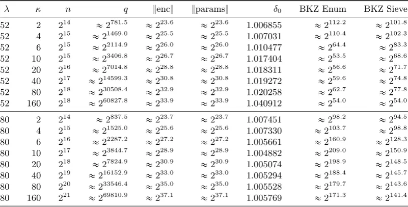
otherwise double n and restart the procedure. We give choices of parameters in Table 2. These tables were produced using the Sage [S`13] module from Appendix A.
λ κ n q }enc} }params} δ0 BKZ Enum BKZ Sieve
52 2 214 «2781.5 «223.6 «223.6 1.006855 «2112.2 «2101.8 52 4 215
«21469.0
«225.5
«225.5 1.007031
«2110.4
«2102.3
52 6 215 «22114.9 «226.0 «226.0 1.010477 «264.4 «283.3 52 10 215
«23406.8
«226.7
«226.7 1.017404
«253.5
«268.6
52 20 216 «27014.8 «228.8 «228.8 1.018311 «256.6 «271.7
52 40 217 «214599.3 «230.8 «230.8 1.019272 «259.6 «274.8
52 80 218 «230508.4 «232.9 «232.9 1.020258 «262.7 «277.8
52 160 218 «260827.8 «233.9 «233.9 1.040912 «254.0 «254.0
80 2 214 «2837.5 «223.7 «223.7 1.007451 «298.2 «294.5 80 4 215
«21525.0
«225.6
«225.6 1.007330
«2103.7
«298.8
80 6 216 «22287.2 «227.2 «227.2 1.005661 «2160.9 «2128.3 80 10 217
«23844.7
«228.9
«228.9 1.004882
«2209.0
«2150.9
80 20 218 «27824.9 «230.9 «230.9 1.005074 «2198.9 «2148.5
80 40 219 «216152.9 «233.0 «233.0 1.005294 «2188.4 «2145.7
80 80 220 «233546.4 «235.0 «235.0 1.005528 «2179.7 «2143.6
80 160 221 «269810.9 «237.1 «237.1 1.005769 «2171.3 «2141.4
Table 2.Parameter choices for multilinear jigsaw puzzles.
5
Implementation
Our implementation relies on FLINT [HJP14]. We use its data types to encode elements in ZrXs, QrXs, and ZqrXs but re-implement most non-trivial operations for the ring of integers
mpfr_t[The13] with precision 2λif not stated otherwise. Our implementation is available under the GPLv2+ license athttps://bitbucket.org/malb/gghlite-flint. We give experimental results for computing multilinear maps using our implementation in Table 1.
For all operations considered in this section naive algorithms are available in O`
n2logq˘ or O`n3logn˘ bit operations. However, the smallest set of parameters we consider in Table 1 is n“215 which implies that if implemented naively each operation would take 249bit operations for the smallest set of parameters we consider. Even quadratic algorithms can be prohibitively expensive. Hence, in order to be feasible, all algorithms should run in quasi-linear time inn, or more precisely inOpnlognqorO`nlog2n˘. All algorithms discussed in this section run in quasi-linear time.
5.1 Polynomial Multiplication inZqrXs{pXn`1q
During the evaluation of a GGH-style graded encoding scheme multiplications of polynomials inZqrXs{pXn`1q are performed. Naive multiplication takesO
`
n2˘time inn, Asymptotically fast multiplication in this ring can be realised by first reducing to multiplication in ZrXs and then to the Sch¨onehage-Strassen algorithm for multiplying large integers in Opnlognlog lognq. This is the strategy implemented in FLINT, which has a highly optimised implementation of the Sch¨onehage-Strassen algorithm. Alternatively, we can get an Opnlognq algorithm by using the Number-Theoretic Transform (NTT). Furthermore, using a negative wrapped convolution we can avoid reductions modulopXn
`1q:
Theorem 1 (Adapted from [Win96]). Letωn be anth root of unity in Zq andϕ2“ωn. Let
a “řni“´01aiXi and b “ř n´1
i“0 biXi P ZqrXs{pXn`1q. Letc “a¨b PZqrXs{pXn`1q and let
a“ pa0, ϕa1, . . . , ϕn´1an´1qand defineb andc analogously. Thenc“1{n¨NTT´
1
ωnpNTTωnpaq d
NTTωnpbqq.
The NTT with a negative wrapped convolution has been used in lattice-based cryptography before, e.g. [LMPR08]. We note that if we are doing many operations inZqrXs{pXn
`1qwe can avoid repeated conversions between coefficient and “evaluation” representations,`fp1q, fpωnq, . . . , fpωn´1 n q
˘ , of our elements, which reduces the amortised cost fromOpnlognqto Opnq. That is, we can con-vert encodings to their evaluation representation once on creation and back only when running extraction. We implemented this strategy. We observe a considerable overall speed-up with the strategy of avoiding the conversions where possible. We also note that operations on elements in their evaluation representation are embarrassingly parallel.
5.2 Computing norms in ZrXs {pXn `1q
During instance generation we have to compute several norms of elements inZrXs {pXn
`1q. The normNpfqof an elementf inZrXs {pXn
`1qis equal to the resultant respf, Xn
`1q. The usual strategy for computing resultants over the integers is to use a multi-modular approach. That is, we compute resultants modulo many small primesqi and then combine the results using the Chinese
Remainder Theorem. Resultants modulo a primeqi can be computed inOpMpnqlognqoperations
whereMpnqis the cost of one multiplication inZqirXs{pX n
`1q. Hence, in our setting computing the norm costsOpnlog2nqoperations without specialisation.
However, we can observe that respf, Xn`1qmodqican be rewritten asśpXn`1qpxq“0fpxqmod
qiasXn`1 is monic, i.e. as evaluatingf on all roots ofXn`1. Pickingqi such thatqi”1 mod 2n
this can be accomplished using the NTT reducing the cost modqi toOpMpnqqsaving a factor of
logn, which in our case is typicallyą15.
5.3 Checking ifpgqis a prime ideal
To check whether the ideal generated byg is prime inZrXs {pXn
`1qwe compute the norm Npgqand check if it is prime which is a sufficient but not necessary condition. However, before computing full resultants, we first check if respg, Xn
`1q “0 modqifor several “interesting” primes
qi. These primes are 2 and then all primes up to some bound with qi ”1 modnbecause these
occur with good probability as factors. We list timings in Table 3.
n logσ wall time n logσ wall time n logσ wall time 1024 15.1 0.54s 2048 16.2 3.03s 4096 17.3 20.99s
Table 3.Average time of checking primality of a singlepgqon Intel Xeon CPU E5–2667 v2 3.30GHz with 256GB of RAM using 16 cores.
5.4 Verifying thatpbp11q, bp21qq “ pgq
If re-randomisation elements are required, then it is necessary that they generate all ofpgq, i.e.
pbp11q, bp21qq “ pgq. Ifbpi1q“˜bip1q¨gfor 0ăiď2 then this condition is equivalent top˜b1p1qq ` p˜bp21qq “R. We check the sufficient but not necessary condition gcdpresp˜bp11q, Xn`1q,resp˜bp21q, Xn`1qq “1, i.e. if the respective ideal norms are co-prime. This check, which we have to perform for every candidate pairp˜bp11q,˜bp21qq, involves computing two resultants and their gcd which is quite expensive. However, we observe that gcdpresp˜bp11q, Xn
`1q,resp˜bp21q, Xn
`1qq ‰1 when resp˜bp11q, Xn
`1q “
0“resp˜bp21q, Xn
`1qmodqi for any modulus qi. Hence, we first check this condition for several
“interesting” primes and resample if this condition holds. These “interesting” primes are the same as in the previous section. Only if these tests pass, we compute two full resultants and their gcd. Indeed, after having ruled out small common prime factors it is quite unlikely that the gcd of the norms is not equal to one which means that with good probability we will perform this expensive step only once as a final verification. However, this step is still by far the most time consuming step during setup even with our optimisations applied. We note that a possible strategy for reducing setup time is to samplemą2 re-randomisersbpi1qand to apply some bounds on the probability of melements ˜bpi1q sharing a prime factor (after excluding small prime factors).
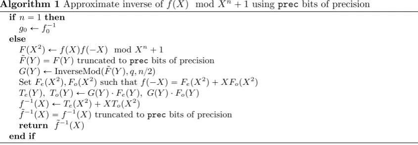
5.5 Computing the inverse of a polynomial modulo Xn `1
Instance generation relies on inversion inQrXs {pXn
`1qin two places. Firstly, when samplingg we have to check that the norm of its inverse is bounded by`g. Secondly, to set up our discrete
Gaussian samplers we need to run many inversions in an iterative process. We note that for computing the zero-testing parameter we only need to invertginZqrXs{pXn`1qwhich can be
realised inninversions in Zq in the NTT representation.
In both cases where inversion inQrXs {pXn`1qis required approximate solutions are sufficient. In the first case we only need to estimate the size ofg´1and in the second case inversion is a
sub-routine of an approximation algorithm (see below). Hence, we implemented a variant of [BCMM98] to compute the approximate inverse of a polynomial inQrXs {pXn`1q, withna power of two.
The core idea is similar to the FFT, i.e. to reduce the inversion of f to the inversion of an element of degree n{2. Indeed, since n is even, fpXqis invertible modulo Xn
`1 if and only if fp´Xqis also invertible. By settingFpX2
q “ fpXqfp´Xq modXn
`1, the inverse f´1 pXqof fpXqsatisfies
FpX2qf´1
pXq “fp´Xq pmodXn`1q. (6)
Let f´1
pXq “ gpXq “ GepX2q `XGopX2q and fp´Xq “ FepX2q `XFopX2q be split into their even and odd parts respectively. From Eq. 6, we obtain FpX2qpGepX2q `XGopX2qq “
FepX2q `XFopX2q pmodXn`1qwhich is equivalent to "
FpX2 qGepX2
q “FepX2
q pmodXn `1q
FpX2 qGopX2
q “FopX2
Algorithm 1Approximate inverse offpXq modXn
`1 usingprecbits of precision if n“1then
g0Ðf0´1
else
FpX2q ÐfpXqfp´Xq modXn`1 ˜
FpYq “FpYqtruncated toprecbits of precision GpYq ÐInverseModpF˜pYq, q, n{2q
SetFepX2
q, FopX2
qsuch thatfp´Xq “FepX2
q `XFopX2
q TepYq, TopYq ÐGpYq ¨FepYq, GpYq ¨FopYq
f´1
pXq ÐTepX2q `XTopX2q ˜
f´1
pXq “f´1
pXqtruncated toprecbits of precision return f˜´1
pXq end if
From this, inverting fpXq can be done by inverting FpX2
q and multiplying polynomials of degree n{2. It remains to recursively call the inversion of FpYq modulo pXn{2
`1q (by setting Y “X2
q. This leads to an algorithm for approximately inverting elements ofQrXs {pXn
`1qwhen nis a power of 2 which can be performed inOpnlog2pnqqoperations inQ. We give experimental results in Table 4.
We give experimental results comparing Algorithm 1 with FLINT’s extended GCD algorithm in Table 4 which highlights that computing approximate inverses instead of exact inverses is necessary for anything but toy instances.
n logσ xgcd 160 160iter 8 4096 17.2 234.1s 0.067s 0.073s 121.8s 8192 18.3 1476.8s 0.195s 0.200s 755.8s
Table 4.InvertinggÐâDZn,σwith FLINT’s extended Euclidean algorithm (“xgcd”), our implementation with precision 160 (“160”), iterating our implementation until }f˜´1
pXq ¨fpXq} ă2´160 (“160iter”) and
our implementation without truncation (“8”) on Intel Core i7–4850HQ CPU at 2.30GHz, single core.
5.6 Small remainders
The Jigsaw Generator as defined in [GGH`13b, Definition 8] takes as input elementsa
iinZpwhere
p“NpIqand produces level encodings with respect to some source groupSi. In particular, this
algorithm produces some small representative of the cosetai modulopgqfrom large integers of size « pσ?nqnif we represents elements inZpas integers 0ďaiăp. This can be accomplished by using
Babai’s trick and thatgis small, i.e. by computingai´g¨tg´1¨aisinQrXs {pXn
`1q. However, in order for this operation to produce sufficiently small elements, we need g´1 either exactly or
with high precision. Computing such a high quality approximation of g´1 can be prohibitively
expensive in terms of memory and time. Our strategy for computing with a lower precision is to rewriteai as
ai“
rlog2paiq{Bs
ÿ
j“0
2B¨j¨aij
where aijă2B for someB. Then, we compute small representatives for all 2B¨j andaij using an
approximation ofg´1with precisionB. Finally, we multiply the small representatives for 2B¨j and
aij and add up their products. This produces a somewhat short element which we then reduce
5.7 Sampling from a Discrete Gaussian
While the strategy in Section 5.6 produces short elements it does not necessarily produce elements which follow a spherical Gaussian distribution and hence do not leak geometric information about g. To produce such samples we need to sample from the discrete Gaussian Dpgq,σ1,c where c is
a small representative of a coset of pgq. Furthermore, if encodings of zero are published, we are required to sample fromDpgq,σ1,0andDpgq,σ1,1. For this, a fundamental building block is to sample
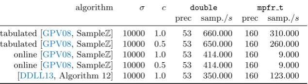
from the integer lattice. We implemented a discrete Gaussian sampler over the integers both in arbitrary precision – using MPFR — and in double precision — using machine doubles. For both cases we implemented rejection sampling from a uniform distribution with and without table (“online”) lookups [GPV08] and Ducas et al’s sampler which samples from DZ,kσ2 whereσ2 is a
constant [DDLL13, Algorithm 12]. Our implementation automatically chooses the best algorithm based onσ,c andτ (the tail cut). In our caseσis typically relatively large, so we call the latter whenever sampling with a centre cPZand the former whencRZ. We list example timings of our discrete Gaussian sampler in Table 5. We note that in our implementation we — conservatively — only make use of the arbitrary precision implementation of this sampler with precision 2λ.
algorithm σ c double mpfr t
prec samp./s prec samp./s tabulated [GPV08, SampleZ] 10000 1.0 53 660.000 160 310.000 tabulated [GPV08, SampleZ] 10000 0.5 53 650.000 160 260.000 online [GPV08, SampleZ] 10000 1.0 53 414.000 160 9.000 online [GPV08, SampleZ] 10000 0.5 53 414.000 160 9.000 [DDLL13, Algorithm 12] 10000 1.0 53 350.000 160 123.000
Table 5.Example timings for discrete Gaussian sampling overZon Intel Core i7–4850HQ CPU at 2.30GHz, single core.
Using our discrete Gaussian sampler over the integers we implemented discrete Gaussian sam-plers over lattices. Implemented naively this takesOpn3logn
qoperations even if we ignore issues of precision. Following [Duc13], we implemented a variant of [Pei10] which we reproduce in Algo-rithm 2. Namely, we first observe thatDpgq,σ1,0“g¨DR,σ1¨g´T and then use [Pei10, Algorithm 1]
to sample fromDR,σ1¨g´T where g´T is the conjugate ofg´1. That is,g0T “g0 and gnT´i “ ´gi
for 1ďiănfor degpgq “n´1. We then proceed as follows. We first compute an approximate square root (see below) ofΣ1
2“g´T ¨g´1up to λbits of precision. We perform operations with
logpnq `4plogp?n}σ}qq bits of precision. If the square root does not converge for this precision, we double it and start over. We then use this value, scaled appropriately, as the initial value from which to start computing a square-root of Σ2 “σ12¨g´T ¨g´1´r2 with r “2¨r
?
logns. We terminate when the square of the approximation is within distance 2´2λ to Σ
2. This typically
happens quickly because our initial candidate is already very close to the target value.
Algorithm 2Computing an approximate square root ofσ12 ¨g´T
¨g´1 ´r2. p, s1Ðlogn`4 logp?n}σ}q, 1
Σ1
2Ðg´T¨g´1
while}s12
´Σ1
2} ą2´λdo
s1
ЫaΣ1
2 computed at prec.puntil}s
12
´Σ2} ă2´λor no more convergence
pÐ2p end while
p, rÐp`2 logσ1, 2¨r?logns Σ2Ðσ¨g´T¨g´1´r2
sЫ?Σ2 computed at precisionpusings1 as initial approximation until}s2´Σ2} ă2´2λ
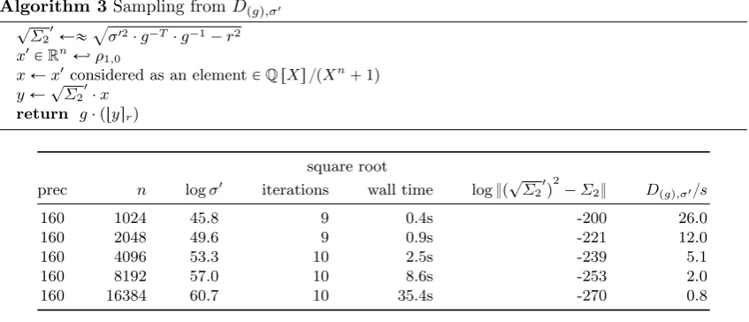
Algorithm 3Sampling fromDpgq,σ1
? Σ2
1
Ыaσ12¨g´T¨g´1´r2
x1
PRnÐâρ1,0
xÐx1considered as an elementP
QrXs {pXn`1q yÐ?Σ2
1 ¨x return g¨ ptysrq
square root
prec n logσ1 iterations wall time log }p?Σ2
1
q2´Σ2} Dpgq,σ1{s
160 1024 45.8 9 0.4s -200 26.0
160 2048 49.6 9 0.9s -221 12.0
160 4096 53.3 10 2.5s -239 5.1
160 8192 57.0 10 8.6s -253 2.0
160 16384 60.7 10 35.4s -270 0.8
Table 6. Approximate square roots ofΣ2 “σ12¨g´T ¨g´r2¨I for discrete Gaussian sampling overg
with parameter σ1 on Intel Core i7–4850HQ CPU at 2.30GHz, 2 cores for Denman-Beavers, 4 cores for estimating the scaling factor, one core for sampling. The last column lists the rate (samples per second) of sampling fromDpgq,σ1.
Given an approximation?Σ2
1
of?Σ2we then sample a vectorxÐâRnfrom a standard normal distribution and interpret it as a polynomial inQrXs {pXn
`1q. We then computey“?Σ2
1
¨xin QrXs {pXn
`1qand returng¨ ptysrq, wheretysr denotes sampling a vector inZn where thei-th component followsDZ,r,yi. This algorithm is then easily extended to sample from arbitrary centres
c. The whole algorithm is summarised in Algorithm 3 and we give experimental results in Table 6.
5.8 Approximate square roots
Our Gaussian sampler requires an (approximate) square root in QrXs {pXn
`1q. That is, for some input element Σ we want to compute some element ?Σ1 P QrXs {pXn `1q such that
}?Σ1¨?Σ1´Σ} ă2´2λ. We use iterative methods as suggested in [Duc13, Section 6.5] which
iteratively refine the approximation of the square root similar to Newton’s method. Computing approximate square roots of matrices is a well studied research area with many algorithms known in the literature (cf. [Hig97]). All algorithms with global convergence invoke approximate inversions inQrXs {pXn
`1qfor which we call our inversion algorithm.
We implemented the Babylonian method, the Denman-Beavers iteration [DB76] and the Pad´e iteration [Hig97]. Although the Babylonian method only involves one inversion which allows us to compute with lower precision, we used Denman-Beavers, since it converges faster in practice and can be parallelised on two cores. While the Pad´e iteration can be parallelised on arbitrarily many cores, the workload on each core is much greater than in the Denman-Beavers iteration and in our experiments only improved on the latter when more than 8 cores were used.
Most algorithms have quadratic convergence but in practice this does not assure rapid con-vergence as error can take many iterations to become small enough for quadratic concon-vergence to be observed. This effect can be mitigated, i.e. convergence improved, by scaling the operands appropriately in each loop iteration of the approximation [Hig97, Section 3]. A common scaling scheme is to scale by the determinant which in our case means computing respf, Xn
`1qfor some f PQrXs {pXn
`1q. Computing resultants in QrXs {pXn
`1qreduces to computing resultants inZrXs pXn
`1q. As discussed above, computing resultants inZrXs {pXn
`1qcan be expensive. However, since we are only interested in an approximation of the determinant for scaling, we can compute with reduced precision. For this, we clear all but the most significant bit for each coefficient’s numerator and denominator off to producef1 and compute res
pf1, Xn
to speed up the resultant computation. With this optimisation scaling by an approximation of the determinant is both fast and precise enough to produce fast convergence. See Table 6 for timings.
Acknowledgement: We would like to thank Guilhem Castagnos, Guillaume Hanrot, Bill Hart, Claude-Pierre Jeannerod, Cl´ement Pernet, Damien Stehl´e, Gilles Villard and Martin Widmer for helpful discussions. We would like to thank Steven Galbraith for pointing out the NTRU-style attack to us and for helpful discussions. This work has been supported in part by ERC Starting Grant ERC-2013-StG-335086-LATTAC. The work of Albrecht was supported by EPSRC grant EP/L018543/1 “Multilinear Maps in Cryptography”.
References
AB15. Benny Applebaum and Zvika Brakerski. Obfuscating circuits via composite-order graded encoding. In Yevgeniy Dodis and Jesper Buus Nielsen, editors,TCC 2015, Part II, volume 9015 ofLNCS, pages 528–556. Springer, March 2015.
APS15. Martin R. Albrecht, Rachel Player, and Sam Scott. On the concrete hardness of learning with errors. Cryptology ePrint Archive, Report 2015/046, 2015. http://eprint.iacr.org/2015/ 046.
BCMM98. Dario Bini, Gianna M. Del Corso, Giovanni Manzini, and Luciano Margara. Inversion of circulant matrices overZm. InProc. of ICALP 1998, volume 1443 ofLNCS, pages 719–730. Springer, 1998.
BF03. Dan Boneh and Matthew Franklin. Identity-based encryption from the Weil pairing. SIAM J. Comput., 32(3):586–615, 2003.
BLR`15. Dan Boneh, Kevin Lewi, Mariana Raykova, Amit Sahai, Mark Zhandry, and Joe Zimmerman. Semantically secure order-revealing encryption: Multi-input functional encryption without obfuscation. In Oswald and Fischlin [OF15b], pages 563–594.
BS03. Dan Boneh and Alice Silverberg. Applications of multilinear forms to cryptography. Contem-porary Mathematics, 324:71–90, 2003.
BWZ14. Dan Boneh, Brent Waters, and Mark Zhandry. Low overhead broadcast encryption from multilinear maps. In Juan A. Garay and Rosario Gennaro, editors,CRYPTO 2014, Part I, volume 8616 ofLNCS, pages 206–223. Springer, August 2014.
CDKD14. Maurice- ´Etienne Cloutier, Jean-Marie De Koninck, and Nicolas Doyon. On the powerful and squarefree parts of an integer. Journal of Integer Sequences, 17(2):28, 2014.
CG13. Ran Canetti and Juan A. Garay, editors. CRYPTO 2013, Part I, volume 8042 of LNCS. Springer, August 2013.
CGH`15. Jean-S´ebastien Coron, Craig Gentry, Shai Halevi, Tancr`ede Lepoint, Hemanta K. Maji, Eric Miles, Mariana Raykova, Amit Sahai, and Mehdi Tibouchi. Zeroizing without low-level zeroes: New MMAP attacks and their limitations. In Gennaro and Robshaw [GR15], pages 247–266. CHL`15. Jung Hee Cheon, Kyoohyung Han, Changmin Lee, Hansol Ryu, and Damien Stehl´e. Crypt-analysis of the multilinear map over the integers. In Oswald and Fischlin [OF15a], pages 3–12.
CLT13. Jean-S´ebastien Coron, Tancr`ede Lepoint, and Mehdi Tibouchi. Practical multilinear maps over the integers. In Canetti and Garay [CG13], pages 476–493.
CLT15. Jean-S´ebastien Coron, Tancr`ede Lepoint, and Mehdi Tibouchi. New multilinear maps over the integers. In Gennaro and Robshaw [GR15], pages 267–286.
CN11. Yuanmi Chen and Phong Q. Nguyen. BKZ 2.0: Better lattice security estimates. In Dong Hoon Lee and Xiaoyun Wang, editors, ASIACRYPT 2011, volume 7073 of LNCS, pages 1–20. Springer, December 2011.
CS97. Don Coppersmith and Adi Shamir. Lattice attacks on NTRU. In Walter Fumy, editor, EUROCRYPT’97, volume 1233 ofLNCS, pages 52–61. Springer, May 1997.
DB76. Eugene D. Denman and Alex N. Beavers Jr. The matrix sign function and computations in systems. Applied Mathematics and Computation, 2:63–94, 1976.
DDLL13. L´eo Ducas, Alain Durmus, Tancr`ede Lepoint, and Vadim Lyubashevsky. Lattice signatures and bimodal gaussians. In Canetti and Garay [CG13], pages 40–56.
Gar13. Sanjam Garg.Candidate Multilinear Maps. PhD thesis, University of California, Los Angeles, 2013.
GGH13a. Sanjam Garg, Craig Gentry, and Shai Halevi. Candidate multilinear maps from ideal lattices. In Thomas Johansson and Phong Q. Nguyen, editors,EUROCRYPT 2013, volume 7881 of LNCS, pages 1–17. Springer, May 2013.
GGH`13b. Sanjam Garg, Craig Gentry, Shai Halevi, Mariana Raykova, Amit Sahai, and Brent Waters. Candidate indistinguishability obfuscation and functional encryption for all circuits. In54th FOCS, pages 40–49. IEEE Computer Society Press, October 2013.
GPV08. Craig Gentry, Chris Peikert, and Vinod Vaikuntanathan. Trapdoors for hard lattices and new cryptographic constructions. In Richard E. Ladner and Cynthia Dwork, editors,40th ACM STOC, pages 197–206. ACM Press, May 2008.
GR15. Rosario Gennaro and Matthew J. B. Robshaw, editors. CRYPTO 2015, Part I, volume 9215 ofLNCS. Springer, August 2015.
Hig97. Nicholas J. Higham. Stable iterations for the matrix square root. Numerical Algorithms, 15(2):227–242, 1997.
HJ15. Yupu Hu and Huiwen Jia. Cryptanalysis of GGH map. Cryptology ePrint Archive, Report 2015/301, 2015. http://eprint.iacr.org/2015/301.
HJP14. William Hart, Fredrik Johansson, and Sebastian Pancratz. FLINT: Fast Library for Number Theory, 2014. Version 2.4.4,http://flintlib.org.
Jou04. Antoine Joux. A one round protocol for tripartite Diffie-Hellman. Journal of Cryptology, 17(4):263–276, September 2004.
LMPR08. Vadim Lyubashevsky, Daniele Micciancio, Chris Peikert, and Alon Rosen. SWIFFT: A modest proposal for FFT hashing. In Kaisa Nyberg, editor,FSE 2008, volume 5086 ofLNCS, pages 54–72. Springer, February 2008.
LP15. Vadim Lyubashevsky and Thomas Prest. Quadratic time, linear space algorithms for Gram-Schmidt orthogonalization and gaussian sampling in structured lattices. In Oswald and Fischlin [OF15a], pages 789–815.
LSS14a. Adeline Langlois, Damien Stehl´e, and Ron Steinfeld. GGHLite: More efficient multilinear maps from ideal lattices. In Phong Q. Nguyen and Elisabeth Oswald, editors,EUROCRYPT 2014, volume 8441 ofLNCS, pages 239–256. Springer, May 2014.
LSS14b. Adeline Langlois, Damien Stehl´e, and Ron Steinfeld. GGHLite: More efficient multilinear maps from ideal lattices. Cryptology ePrint Archive, Report 2014/487, 2014. http://eprint. iacr.org/2014/487.
OF15a. Elisabeth Oswald and Marc Fischlin, editors. EUROCRYPT 2015, Part I, volume 9056 of LNCS. Springer, April 2015.
OF15b. Elisabeth Oswald and Marc Fischlin, editors. EUROCRYPT 2015, Part II, volume 9057 of LNCS. Springer, April 2015.
Pei10. Chris Peikert. An efficient and parallel gaussian sampler for lattices. In Tal Rabin, editor, CRYPTO 2010, volume 6223 ofLNCS, pages 80–97. Springer, August 2010.
S`13. William Stein et al. Sage Mathematics Software Version 6.2. The Sage Development Team, 2013. Available athttp://www.sagemath.org.
SE94. C. P. Schnorr and M. Euchner. Lattice basis reduction: Improved practical algorithms and solving subset sum problems. Mathematical Programming, 66(1-3):181–199, 1994.
The13. The MPFR team. GNU MPFR: The Multiple Precision Floating-Point Reliable Library, 3.1.2 edition, 2013. http://www.mpfr.org/.
Win96. Franz Winkler. Polynomial Algorithms in Computer Algebra. Texts and Monographs in Symbolic Computation. Springer, 1996.
Zim15. Joe Zimmerman. How to obfuscate programs directly. In Oswald and Fischlin [OF15b], pages 439–467.
A
Parameter Estimation Source Code
# * c o d i n g : utf 8 *
-f r o m c o l l e c t i o n s i m p o r t O r d e r e d D i c t f r o m c o p y i m p o r t c o p y
f r o m s a g e . f u n c t i o n s . o t h e r i m p o r t s q r t f r o m s a g e . m i s c . m i s c i m p o r t g e t _ v e r b o s e f r o m s a g e . r i n g s . all i m p o r t ZZ , RR , R e a l F i e l d f r o m s a g e . s y m b o l i c . all i m p o r t pi , e
# U t i l i t y F u n c t i o n s
def p a r a m s _ s t r ( d , k e y w o r d _ w i d t h = N o n e ) : """
R e t u r n s t r i n g of key , v a l u e p a i r s as a s t r i n g " k e y 0 : value0 , k e y 1 : v a l u e 1 "
: p a r a m d : r e p o r t d i c t i o n a r y
: k e y w o r d _ w i d t h : k e y s are p r i n t e d w i t h t h i s w i d t h """
if d is N o n e : r e t u r n s = [] for k in d :
v = d [ k ]
if k e y w o r d _ w i d t h :
fmt = u " %%% ds " % k e y w o r d _ w i d t h k = fmt % k
if ZZ (1) / 2 0 4 8 < v < 2 0 4 8 or v == 0: try :
s . a p p e n d (u " % s : %9 d " % ( k , ZZ ( v ) ) ) e x c e p t T y p e E r r o r :
if v < 2.0 and v >= 0 . 0 :
s . a p p e n d (u " % s : % 9 . 7 f " % ( k , v ) ) e l s e :
s . a p p e n d (u " % s : % 9 . 4 f " % ( k , v ) ) e l s e :
t = u "«2 ^ % . 1 f " % log ( v , 2) . n () s . a p p e n d (u " % s : %9 s " % ( k , t ) ) r e t u r n u " , ". j o i n ( s )
def p a r a m s _ r e o r d e r ( d , o r d e r i n g ) : """
R e t u r n a new o r d e r e d d i c t f r o m the key : v a l u e p a i r s in ‘d ‘ but r e o r d e r e d s u c h t h a t the k e y s in o r d e r i n g c o m e f i r s t .
: p a r a m d : i n p u t d i c t i o n a r y
: p a r a m o r d e r i n g : k e y s w h i c h s h o u l d c o m e f i r s t ( in o r d e r )
"""
k e y s = l i s t ( d ) for key in o r d e r i n g :
k e y s . pop ( k e y s . i n d e x ( key ) ) k e y s = l i s t ( o r d e r i n g ) + k e y s r = O r d e r e d D i c t ()
for key in k e y s : r [ key ] = d [ key ] r e t u r n r
# L a t t i c e R e d u c t i o n E s t i m a t e s
def k _ c h e n ( d e l t a ) : """
E s t i m a t e r e q u i r e d b l o c k s i z e ‘k ‘ for a g i v e n root - h e r m i t e f a c t o r δ_0 .
: p a r a m d e l t a : root - h e r m i t e f a c t o r δ_0 """
k = ZZ ( 4 0 )
RR = d e l t a . p a r e n t () p i _ r = RR ( pi ) e_r = RR ( e )
f = l a m b d a k : ( k / ( 2 * p i _ r * e_r ) * ( p i _ r * k ) * * ( 1 / k ) ) * * ( 1 / ( 2 * ( k -1) ) )
w h i l e f (2* k ) > d e l t a : k *= 2
w h i l e f ( k + 1 0 ) > d e l t a : k += 10
w h i l e T r u e :