Faster Compact Diffie–Hellman:
Endomorphisms on the
x
-line
Craig Costello1, Huseyin Hisil2, and Benjamin Smith3,4 1
Microsoft Research, Redmond, USA [email protected] 2
Yasar University, Izmir, Turkey [email protected] 3
INRIA (´Equipe-projet GRACE), France 4
LIX (Laboratoire d’Informatique), ´Ecole polytechnique, France [email protected]
Abstract. We describe an implementation of fast elliptic curve scalar multiplication, optimized for Diffie–Hellman Key Exchange at the 128-bit security level. The algorithms are compact (using only x-coordinates), run in constant time with uniform execution patterns, and do not distinguish between the curve and its quadratic twist; they thus have a built-in measure of side-channel resistance. (For comparison, we also implement two faster but non-constant-time algorithms.) The core of our construction is a suite of two-dimensional differential addition chains driven by efficient endomorphism decompositions, built on curves selected from a family of Q-curve reductions over Fp2 with p = 2127 −1. We include state-of-the-art experimental results for twist-secure, constant-time,x-coordinate-only scalar multiplication.
Keywords: Elliptic curve cryptography, scalar multiplication, twist-secure, side channel attacks, endomorphism, Kummer variety, addition chains, Montgomery curve.
1
Introduction
In this paper, we discuss the design and implementation of state-of-the-art Elliptic Curve Diffie– Hellman key exchange (ECDH) primitives for security level of approximately 128 bits. The major priorities for our implementation are
1. Compactness: We targetx-coordinate-only systems. These systems offer the advantages of shorter keys, simple and fast algorithms, and (when properly designed) the use of arbitrary x-values, not just legitimate x-coordinates of points on a curve (the “illegitimate” values are x-coordinates on the quadratic twist). For x-coordinate ECDH, the elliptic curve exists only to supply formulæ for scalar multiplications, and a hard elliptic curve discrete logarithm problem (ECDLP) to underwrite a hard computational Diffie–Hellman problem (CDHP) on x-coordinates. The users should not have to verify whether given values correspond to points on a curve, nor should they have to compute any quantity that cannot be derived simply from x-coordinates alone. In particular, neither a user nor an algorithm should have to distinguish between the curve and its quadratic twist—and the curve must be chosen to be twist-secure. 2. Fast, constant-time execution: Every Diffie–Hellman key exchange is essentially comprised
of four scalar multiplications,5 so optimizing scalar multiplicationP 7→ [m]P for varying P andmis a very high priority. At the same time, a minimum requirement for protecting against side-channel timing attacks is that every scalar multiplicationP 7→[m]P must be computed in constant time (and ideally with the same execution pattern), regardless of the values ofm and P.
†This is the full version of the article to appear in EUROCRYPT 2014, LNCS, Vol. 8441, cIACR. 5
Our implementation targets a security level of approximately 128 bits (comparable with
Curve25519[3],secp256r1[12], andbrainpoolP256t1[22]). The reference system with respect to our desired properties is Bernstein’sCurve25519, which is based on an efficient, uniform differential addition chain applied to a well-chosen pair of curve and twist presented as Montgomery models. These models not only provide highly efficient group operations, but they are optimized for x -coordinate-only operations, which (crucially) do not distinguish between the curve and its twist. Essentially, well-chosen Montgomery curves offer compactness straight out of the box.
Having chosen Montgomery curves as our platform, we must implement a fast, uniform, and constant-time scalar multiplication on their x-coordinates. To turbocharge our scalar multiplication, we apply a combination of efficiently computable pseudo-endomorphisms and two-dimensional differential addition chains. The use of efficient endomorphisms follows in the tradition of [21], [34], [16], and [15], but to the best of our knowledge, this work represents the first use of endomorphism scalar decompositions in thepure x-coordinate setting (that is, without additional input to the addition chain).
Our implementation is built on a curve-twist pair (E,E′
) equipped with efficiently computable endomorphisms (ψ, ψ′
). The family of Q-curve reductions in [33] offer a combination of fast endomorphisms and compatibility with fast underlying field arithmetic. Crucially (and unlike earlier endomorphism constructions such as [16] and [15]), they also offer the possibility of twist-secure group orders over fast fields. One of these curves, with almost-prime order over a 254-bit field, forms the foundation of our construction (see §2). Any other curve from the same family over the same field could be used with only very minor modifications to the formulæ below and the source code for our implementations; we explain our specific curve choice in Appendix B. The endomorphisms ψ and ψ′ induce efficient pseudo-endomorphisms ψ
x and ψ′x on the x-line; we
explain their construction and use in§3.
The key idea of this work is to replace conventional scalar multiplications (m, x(P))7→x([m]P) with multiscalar multiexponentiations
((a, b), x(P))7−→x([a]P⊕[b]ψ(P)) orx([a]P⊕[b]ψ′
(P)),
where (a, b) is either a short multiscalar decomposition of a random full-length scalarm(that is, such that [m]P = [a]P⊕[b]ψ(P) or [a]P⊕[b]ψ′
(P)), or a random short multiscalar. The choice of ψorψ′
formally depends on whetherP is onE orE′
, but there is no difference betweenψandψ′
on the level ofx-coordinates: they are implemented using exactly the same formulæ. Since every element of the base field is thex-coordinate of a point onEorE′
, we may view the transformation above as acting purely on field elements and not curve points.
From a practical point of view, the two crucial differences compared with conventional ECDH over a 254-bit field are
1. The use of 128-bit multiscalars (a, b) inZ2 in place of the 254-bit scalarm in Z. We treat the geometry of multiscalars, the distribution of their corresponding scalar values, and the derivation of constant-bitlength scalar decompositions in§4.
2. The use of two-dimensional differential addition chainsto compute x([a]P ⊕[b]ψ(P)) given only (a, b) andx(P). We detail this process in§5.
We have implemented three different two-dimensional differential addition chains: one due to Montgomery [25] via Stam [35], one due to Bernstein [4], and one due to Azarderakhsh and Karabina [1]. Each offers a different combination of speed, uniformity, and constant-time execution. We provide implementation details and timings for scalar multiplications based on each chain in§6. The differential nature of these chains is essential in thex-coordinate setting, which prevents the effective use of the vector chains traditionally used in the endomorphism literature (such as [36]).
A Magma implementation is publicly available at
http://research.microsoft.com/en-us/downloads/ef32422a-af38-4c83-a033-a7aafbc1db55/ ;
a complete mixed-assembly-and-C implementation6is publicly available (in eBATS [9] format) at http://hhisil.yasar.edu.tr/files/hisil20140318compact.tar.gz .
6
2
The Curve
We begin by defining our curve-twist pair (E,E′
). We work over
Fp2:=Fp(i), where p:= 2127−1 and i2=−1 .
We chose this Mersenne prime for its compatibility with a range of fast techniques for modular arithmetic, including Montgomery- and NIST-style approaches. We build efficientFp2-arithmetic on top of the fastFp-arithmetic described in [11]. Appendix A provides a complete description of our arithmetic routines.
In what follows, it will be convenient to define the constants u:= 1466100457131508421, v:= 1
2(p−1) = 2
126−1, w:= 1
4(p+ 1) = 2 125.
The Curve E and its Twist E′. We define E to be the elliptic curve over F
p2 with affine Montgomery model
E:y2=x(x2+Ax+ 1), where
A=A0+A1·i with
A0= 45116554344555875085017627593321485421, A1= 2415910908.
The element 12/Ais not a square inFp2, so the curve overFp2 defined by
E′ : (12/A)y2=x(x2+Ax+ 1)
is a model of the quadratic twist of E. The twisting Fp4-isomorphism δ : E → E′ is defined by δ : (x, y) 7→ (x,(A/12)1/2y). The mapδ
1 : (x, y) 7→ (xW, yW) = (12Ax+ 4,12
2
A2y) defines an
Fp2-isomorphism betweenE′ and the Weierstrass model
E2,−1,s:y2W =xW3 + 2(9(1 +si)−24)xW −8(9(1 +si)−16)
of [33, Theorem 1] with
s=i(1−8/A2) = 86878915556079486902897638486322141403,
soE is a Montgomery model of the quadratic twist ofE2,−1,s. (In the notation of [33,§5] we have E ∼=E′
2,−1,s andE
′∼
=E2,−1,s.) These curves all havej-invariant
j(E) =j(E′) =j(E2,−1,s) = 28(A
2−3)3 A2−4 = 2
6(5−3si)3(1−si) (1 +s2)2 .
Group Structures. Using the SEA algorithm [29], we find that #E(Fp2) = 4N and #E′(Fp2) = 8N′ where
N =v2+ 2u2 and N′
= 2w2−u2 are 252-bit and 251-bit primes, respectively. Looking closer, we see that
E(Fp2)∼= (Z/2Z)2×Z/NZ and E′(Fp2)∼=Z/2Z×Z/4Z×Z/N′Z.
Recall that every element ofFp2is either thex-coordinate of two points inE(Fp2), thex-coordinate of two points inE′
(Fp2), or thex-coordinate of one point of order two in bothE(Fp2) andE′(Fp2). The x-coordinates of the points of exact order 2 in E(Fp2) (and in E′(Fp2)) are 0 and −12A±
1 2
√
A2−4; the points of exact order 4 inE′(F
p2) havex-coordinates±1. Either of the points with x-coordinate 2 will serve as a generator for the cryptographic subgroup E(Fp2)[N]; either of the points withx-coordinate 2−igenerateE′(F
Curve Points, x-Coordinates, and Random Bitstrings. Being Montgomery curves, both
E andE′ are compatible with the Elligator 2 construction [6,
§5]. For our curves, [6, Theorem 5] defines efficiently invertible injective mapsFp2 → E(Fp2) andFp2→ E′(Fp2). This allows points on
E and/orE′ to be encoded in such a way that they are indistinguishable from uniformly random
254-bit strings. Since we work withx-coordinates only in this article, a square root is saved when computing the injection (see [6,§5.5] for more details).
The ECDLP on E and E′. Suppose we want to solve an instance of the DLP in E(F
p2) or
E′
(Fp2). Applying the Pohlig–Hellman–Silver reduction [26], we almost instantly reduce to the case of solving a DLP instance in eitherE(Fp2)[N] or E′(Fp2)[N′]. The best known approach to solving such a DLP instance is Pollard’s rho algorithm [27], which (properly implemented) can solve DLP instances inE(Fp2)[N] (resp.E′(Fp2)[N′]) in around 12
√
πN ∼2125.8(resp. 1 2
√
πN′
∼2125.3) group operations on average [10]. One might expect that working overFp2would imply a
√
2-factor speedup in the rho method by using Frobenius classes; but this seems not to be the case, since neitherE norE′
is a subfield curve [37,§6]. The embedding degrees ofE andE′
with respect to N andN′
are 501(N−1) and 12(N′
−1), respectively, so ECDLP instances inE(Fp2)[N] andE(Fp2)[N′] are not vulnerable to the Menezes– Okamoto–Vanstone [23] or Frey–R¨uck [14] attacks. The trace ofEisp2+ 1−4N6=±1, so neither
E norE′
are amenable to the Smart–Satoh–Araki–Semaev attack [28], [30], [31].
While our curves are defined over a quadratic extension field, this does not seem to reduce the expected difficulty of the ECDLP when compared with elliptic curves over similar-sized prime fields. Taking the Weil restriction ofE (orE′) toF
p as in the Gaudry–Hess–Smart attack [18], for
example, produces a simple abelian surface overFp; and the best known attacks on DLP instances
on simple abelian surfaces overFp offer no advantage over simply attacking the ECDLP on the
original curve (see [32], [17], and [15,§9] for further discussion).
Superficially,E is what we would normally call twist-secure (in the sense of Bernstein [3] and Fouque–R´eal–Lercier–Valette [13]), since its twist E′
has a similar security level. Indeed, E (and the whole class of curves from which it was drawn) was designed with this notion of twist-security in mind. However, twist-security is more subtle in the context of endomorphism-based scalar decompositions; we will return to this subject in§4 below.
The Endomorphism Ring. Let πE denote the Frobenius endomorphism of E. The curve E is
ordinary (its tracetE is prime to p), so its endomorphism ring is an order in the quadratic field
K :=Q(πE). (The endomorphism ring of an ordinary curve and its twist are always isomorphic,
so what holds below for E also holds for E′.) We will see below that
E has an endomorphismψ such thatψ2=−[2]π
E. The discriminant ofZ[ψ] is the fundamental discriminant
DK =−8·5·397·10528961·6898209116497·1150304667927101
ofK, soZ[ψ] is the maximal order inK; hence, End(E) =Z[ψ].
Thesafecurvesspecification [8] suggests that the discriminant of the CM field should have at least 100 bits; ourE easily meets this requirement, since DK has 130 bits. We note that
well-chosen GLS curves can also have large CM field discriminants, but GLV curves have tiny CM field discriminants by construction: for example, the endomorphism ring of the curvesecp256k1[12] (at the heart of the Bitcoin system) has discriminant−3.
Brainpool[22] requires the ideal class number of K to be larger than 107; this property is never satisfied by GLV curves, which have tiny class numbers (typically≤2) by construction. But
E easily meets this requirement: the class number of End(E) is
3
Efficient Endomorphisms on
E
,
E
′, and the
x
-line
Theorem 1 of [33] defines an efficient endomorphism
ψ2,−1,s: (xW, yW)7−→
−xpW
2 −
9(1−si) xpW −4 ,
yWp
√ −2
−1
2 +
9(1−si) (xpW −4)2
of degree 2pon the Weierstrass modelE2,−1,s, with kernel h(4,0)i. To avoid an ambiguity in the
sign of the endomorphism, we must fix a choice of√−2 inFp2. We choose the “small” root:
√
−2 := 264·i . (1)
Applying the isomorphismsδandδ1, we define efficientFp2-endomorphisms ψ:= (δ1δ)−1ψ2,−1,sδ1δ and ψ′:=δψδ−1=δ1−1ψ2,−1,sδ1 of degree 2ponE and E′, respectively, each with kernel
h(0,0)i. More explicitly: if we let n(x) := AAp x2+Ax+ 1
, d(x) :=−2x , s(x) :=n(x)p/d(x)p , r(x) := Ap
A(x
2−1), and m(x) :=n′
(x)d(x)−n(x)d′
(x), thenψandψ′
are defined (using the same value of√−2 fixed in Eq. (1)) by
ψ: (x, y)7−→
s(x), −12
v
Av√−2
ypm(x)p
d(x)2p
and
ψ′
: (x, y)7−→
s(x), −12 2v√−2
A2v
ypr(x)p
d(x)2p
.
Actions of the Endomorphisms on Points. Theorem 1 of [33] tells us that
ψ2=−[2]πE and (ψ′)2= [2]πE′ , (2) whereπE andπE′ are thep2-power Frobenius endomorphisms ofE andE′, respectively, and
P(ψ) =P(ψ′) = 0, where P(T) =T2−4uT + 2p .
If we restrict to the cryptographic subgroup E(Fp2)[N], then ψ must act as multiplication by an integer eigenvalueλ, which is one of the two roots ofP(T) modulo N. Similarly, ψ′
acts on
E′
(Fp2)[N′] as multiplication by one of the rootsλ′ ofP(T) moduloN′. The correct eigenvalues are
λ≡ −uv (modN) and λ′ ≡ −2uw (modN′). Equation (2) implies thatλ2≡ −2 (modN) andλ′2
≡2 (modN′
). (Note that choosing the other square root of−2 in Eq. (1) negatesψ, ψ′
,λ,λ′
, andu.)
To complete our picture of the action ofψonE(Fp2) andψ′ onE′(Fp2), we describe its action on the points of order 2 and 4 listed above:
(0,0) 7−→ 0 underψandψ′ ,
−1 2A±
1 2
√
A2−4,0
7−→ (0,0) underψandψ′ ,
1,±21
p
A(A+ 2)/3
7−→ −12A− 1 2
√
A2−4,0
underψ′
,
−1,±12
p
−A(A+ 2)/3
7−→ −12A+ 1 2
√
A2−4,0
underψ′
Pseudo-endomorphisms on the x-line. One advantage of the Montgomery model is that it allows a particularly efficient arithmetic using only the x-coordinate. Technically speaking, this corresponds to viewing thex-lineP1 as the Kummer variety ofE: that is,P1∼=E/h±1i.
The x-line is not a group: if P and Q are points on E, then x(P) and x(Q) determine the pair {x(P ⊕Q), x(P⊖Q)}, but not the individual elements x(P ⊕Q) and x(P ⊖Q). However, thex-line inherits part of the endomorphism structure ofE: every endomorphismφof E induces a pseudo-endomorphism7φ
x:x7→φx(x) of P1, which determines φup to sign; and ifφ1and φ2 are two endomorphisms ofE, then
(φ1)x(φ2)x= (φ2)x(φ1)x= (φ1φ2)x= (φ2φ1)x.
Montgomery’s explicit formulæ for pseudo-doubling (DBL), pseudo-addition (ADD), combined pseudo-doubling and pseudo-addition (DBLADD) on P1 are available in [7]. In addition to these, we need expressions for both ψx and (ψ±1)x to initialise the addition chains in §5. Moving to
projective coordinates: writex=X/Z andy =Y /Z. Then the negation map on E is [−1] : (X : Y :Z)7→(X :−Y :Z), and the double coverE → E/h[±1]i ∼=P1is (X :Y :Z)7→(X :Z). The pseudo-doubling onP1 is
[2]x((X:Z)) = (X+Z)2(X−Z)2: (4XZ) (X−Z)2+A+24 ·4XZ . (3)
Our endomorphism ψinduces the pseudo-endomorphism
ψx((X :Z)) =
Ap (X−Z)2−A+22 (−2XZ)
p
:A(−2XZ)p .
Composingψx with itself, we confirm thatψxψx=−[2]x(πE)x.
Proposition 1. With the notation above, and with√−2 chosen as in Eq.(1),
(ψ±1)x(x) = (ψ′±1)x(x)
= 2s
2nd4p−x(xn)pm2pAp−1 2s(x−s)2d4pAp−1 ∓
mp(xn)(p+1)/2√−2
A(p−1)/2(x−s)2d2p . (4)
Proof. IfP andQare points on a Montgomery curveBy2=x(x2+Ax+ 1), then
x(P ±Q) = B(x(P)y(Q)∓x(Q)y(P)) 2
x(P)x(Q) (x(P)−x(Q))2 .
TakingP= (x, y) to be a generic point onE (whereB= 1), settingQ=ψ(P), and eliminating y usingy2=−Ap
2Adnyields the expression for (ψ±1)xabove. The same process forE
′
(withB= 12A), eliminatingy with 12Ay2=−Ap
2Adn, yields the same expression for (ψ
′
±1)x. ⊓⊔
Deriving explicit formulæ to compute the pseudo-endomorphism images in Eq. (4) is straightforward. We omit these formulæ here for space considerations, but they can be found in our code online. IfP ∈ E, then on input ofx(P), the combined computation of the three projective elements (Xλ−1:Zλ−1), (Xλ:Zλ), (Xλ+1:Zλ+1), which respectively correspond to the three affine
elementsx([λ−1]P),x([λ]P),x([λ+1]P), incurs 15 multiplications, 129 squarings and 10 additions in Fp2. The bottleneck of this computation is raisingdnto the power of (p+ 1)/2 = 2126, which incurs 126 squarings. We note that squarings are significantly faster than multiplications in Fp2 (see Appendix A).
7 “Pseudo-endomorphisms” are true endomorphisms of
4
Scalar Decompositions
We want to evaluate scalar multiplications [m]P as [a]P⊕[b]ψ(P), where m≡a+bλ (mod N)
and the multiscalar (a, b) has a significantly shorter bitlength8 than m. For our applications we impose two extra requirements on multiscalars (a, b), so as to add a measure of side-channel resistance:
1. both aandbmust bepositive, to avoid branching and to simplify our algorithms; and 2. the multiscalar (a, b) must haveconstant bitlength(independent ofmas mvaries overZ),
so that multiexponentiation can run in constant time.
In some protocols—notably Diffie–Hellman—we are not interested in the particular values of our random scalars, as long as those values remain secret. In this case, rather than starting with m in Z/NZ (orZ/N′Z
) and finding a short, positive, constant-bitlength decomposition of m, it would be easier to randomly sample some short, positive, constant-bitlength multiscalar (a, b) from scratch. The sample space must be chosen to ensure that the corresponding distribution of values a+bλinZ/NZdoes not make the discrete logarithm problem of findinga+bλappreciably easier than if we started with a randomm.
Zero Decomposition Lattices. The problems of finding good decompositions and sampling good multiscalars are best addressed using the geometric structure of the spaces of decompositions forEandE′. The multiscalars (a, b) such thata+bλ
≡0 (modN) ora+bλ′
≡0 (mod N′) form
lattices
L=h(N,0),(−λ,1)i and L′
=h(N′
,0),(−λ′
,1)i ,
respectively, witha+bλ≡c+dλ (modN) if and only if (a, b)−(c, d) is inL(similarly,a+bλ′
≡
c+dλ′
(modN′
) if and only if (a, b)−(c, d) is inL′
).
The sets of decompositions ofmforE(Fp)[N] and E(Fp2)[N′] therefore form lattice cosets (m,0) +L and (m,0) +L′
,
respectively, so we can compute short decompositions of m for E(Fp)[N] (resp. E(Fp2)[N′]) by subtracting vectors near (m,0) inL(resp.L′) from (m,0). To find these vectors, we need
k · k∞
-reduced9bases forL andL′.
Proposition 2 (Definition of e1,e2,e′
1,e
′
2). Up to order and sign, the shortest possible bases
for L andL′
(with respect to k · k∞) are given by
L=he1:= (v, u) , e2:= (−2u, v)i and
L′
=he′
1:= (u, w) , e
′
2:= (2u−2w,2w−u)i.
Proof. The proof of [33, Prop. 2] constructs sublattices
h˜e1:=−2(v, u),˜e2:=−2(2u, v)i ⊂ L
and
h˜e′
1:= 2(2w,−u),e˜
′
2:= 4(u, w)i ⊂ L
′
with [L:h˜e1,˜e2i] = 4 and [L′
:he˜′
1,˜e
′
2i] = 8. We easily verify thate1=−12˜e2 ande2=− 1 2˜e1 are both inL; then, sinceh˜e1,e2˜ ihas index 4 inhe1,e2i, we must haveL=he1,e2i. Similarly, both
8
The bitlength of a scalarmis⌈log2|m|⌉; the bitlength of a multiscalar (a, b) is⌈log2k(a, b)k∞⌉. 9
e′
1=14˜e
′
2ande
′
2=12(˜e
′
2−˜e
′
1) are inL
′, and thus form a basis for
L′. According to [20, Definition
3], an ordered lattice basis [b1,b2] isk · k∞-reduced if
kb1k∞≤ kb2k∞≤ kb1−b2k∞≤ kb1+b2k∞ .
This holds for [b1,b2] = [e2,−e1] and [e′
1,e′2], soke2k∞andke1k∞(resp.ke′1k∞andke′2k∞) are
the successive minima ofL(resp.L′) by [20, Theorem 5].10 ⊓⊔ In view of Proposition 2, the fundamental parallelograms of L and L′
are the regions of the (a, b)-plane defined by
A:=
(a, b)∈R2 : 0≤vb−ua < N, 0≤2ub+va < N and
A′:=
(a, b)∈R2 : 0≤ub−wa < N′, 0≤(2u−2w)b−(2w−u)a < N′ ,
respectively. Every integermhas precisely one decomposition forE(Fp2)[N] (resp.E′(Fp2)[N′]) in any translate ofAbyL (resp.A′
byL′
).
Short, Constant-Bitlength Scalar Decompositions. Returning to the problem of finding short decompositions ofm: let (α, β) be the (unique) solution in Q2 to the systemαe1+βe2 = (m,0). Sincee1,e2 is reduced, the closest vector to (m,0) inLis one of the four vectors⌊α⌋e1+
⌊β⌋e2,⌊α⌋e1+⌈β⌉e2,⌈α⌉e1+⌊β⌋e2, or⌈α⌉e1+⌈β⌉e2by [20, Theorem 19]. Following Babai [2], we subtract⌊α⌉e1+⌊β⌉e2 from (m,0) to get a decomposition (˜a,˜b) ofm; by the triangle inequality,
k(˜a,˜b)k∞ ≤ 12(ke1k∞+ke2k∞). This decomposition is approximately the shortest possible, in
the sense that the true shortest decomposition is at most±e1±e2away. Observe thatke1k∞=
ke2k∞= 2126−1, so (˜a,˜b) has bitlength at most 126.
However, ˜a or ˜b may be negative (violating the positivity requirement), or have fewer than 126 bits (violating the constant bitlength requirement). Indeed, m 7→ (˜a,˜b) maps Z onto (A −
1
2(e1+e2))∩Z2. This region of the (a, b)-plane, “centred” on (0,0), contains multiscalars of every bitlength between 0 and 126—and the majority of them have at least one negative component. We can achieve positivity and constant bitlength by adding a carefully chosen offset vector from
L, translating (A − 1
2(e1+e2))∩Z
2 into a region of the (a, b)-plane where every multiscalar is positive and has the same bitlength. Adding 3e1or 3e2ensures that the first or second component always has precisely 128 bits, respectively; but adding 3(e1+e2) gives us a constant bitlength of 128 bits in both. Theorem 1 makes this all completely explicit.
Theorem 1. Given an integerm, let (a, b)be the multiscalar defined by
a:=m+ (3− ⌊α⌉)v−2 (3− ⌊β⌉)u and b:= (3− ⌊α⌉)u+ (3− ⌊β⌉)v ,
whereαandβ are the rational numbers
α:= (v/N)m and β :=−(u/N)m .
Then2127< a, b <2128, andm≡a+bλ (modN). In particular,(a, b)is a positive decomposition
of m, of bitlength exactly 128, for anym.
Proof. We havem≡a+bλ (mod N) because (a, b) = (˜a,˜b) + 3(e1+e2)≡(m,0) (mod L), where (˜a,˜b) is the translate of (m,0) by the Babai roundoff⌊α⌉e1+⌊β⌉e2 described above. Now (˜a,˜b) lies in A −1
2(e1+e2), so (a, b) lies in A+ 5
2(e1,e2); our claim on the bitlength of (a, b) follows because the four “corners” of this domain all have 128-bit components. ⊓⊔
10
Random Multiscalars. As we remarked above, in a pure Diffie–Hellman implementation it is more convenient to simply sample random multiscalars than to decompose randomly sampled scalars. Proposition 3 shows that random multiscalars of at most 127 bits correspond to reasonably well-distributed values in Z/NZ and in Z/N′Z, in the sense that none of the values occur more
than one more or one fewer times than the average, and the exceptional values are in O(√N). Such multiscalars can be trivially turned into constant-bitlength positive 128-bit multiscalars— compatible with our implementation—by (for example) completing a pair of 127-bit strings with a 1 in the 128-th bit position of each component.
Proposition 3. Let B= [0, p]2; we identify Bwith the set of all pairs of strings of 127 bits.
1. The mapB →Z/NZdefined by(a, b)7→a+bλ (modN)is 4-to-1, except for4(p−6u+ 4)≈
4√2N values in Z/NZ with 5 preimages in B, and 8(u2−3u+ 2)≈ 1 5
√
N values in Z/NZ
with only 3 preimages inB. 2. The mapB →Z/N′Z
defined by (a, b)7→a+bλ′
(mod N′
)is 8-to-1, except for8u2≈ 2 7
√
N′
values with 9 preimages in B.
Proof (Sketch).For (1): the map (a, b)7→a+bλ (mod N) defines a bijection between each translate ofA ∩Z2byLandZ/NZ. Hence, everyminZ/NZhas a unique preimage (a
0, b0) inA ∩Z2, so it suffices to count ((a0, b0)+L)∩Bfor each (a0, b0) inA∩Z2. CoverZ2with translates ofAbyL; the only points inZ2that are on the boundaries of tiles are the points inL. DissectingBalong the edges of translates ofAand reassembling the pieces, we see that 8v−24u+20<4pmultiscalars inBoccur with multiplicity five, 8u2−24u+ 16< p/9 with multiplicity three, and every other multiscalar occurs with multiplicity four. There are therefore 4N+ (8v−24u+ 20)−(8u2−24u+ 16) = (p+ 1)2 preimages in total, as expected. The proof of (2) is similar to (1), but counting ((a, b) +L′)
∩ Bas (a, b) ranges overA′.
⊓ ⊔
We note that in our online C code, the decomposition of the scalark into k0 and k1 is not implemented in constant time. Although there are known methods of achieving this, samplingk0 andk1at random is certainly easier: in our code, these multiscalars can be selected at random by simply commenting out the ‘#define DECOMPOSITION’ line.
Twist-Security with Endomorphisms. We saw in §2 that DLPs on E and its twist E′
have essentially the same difficulty, while Proposition 3 shows that the real DLP instances presented to an adversary by 127-bit multiscalar multiplications are not biased into a significantly more attackable range. But there is an additional subtlety when we consider the fault attacks considered in [3] and [13]: If we try to compute [m]P forP onE, but an adversary sneaks in a pointP′
on the twistE′instead, then in the classical context the adversary can derivemafter solving the discrete
logarithm [m modN′]P′ in
E′(F
p2). But in the endomorphism context, we compute [m]P as [a]P ⊕[b]ψ(P), and the attacker sees [a+bλ′]P′, which is not [m modN′]P′ (or even [a+bλ
modN′]P′); we should ensure that the values (a+bλ′ modN′) are not concentrated in a small
subset ofZ/N′Zwhen (a, b) is a decomposition for
E(Fp2)[N]. This can be achieved by a similar argument to that of Proposition 3: the map Z/NZ → Z/N′Z defined by m
7→ (a, b)7→ a+bλ′
(modN′) is a good approximation of a 2-to-1 mapping.
5
Two-Dimensional Differential Addition Chains
Montgomery ladder is in the form [i]P⊕[i+1]P, so every associated difference is equal toP. Several two-dimensional differential addition chains have been proposed, targeting multiexponentiations in elliptic curves and other primitives; we suggest [4] and [35] for overviews.
In any two-dimensional differential chain computing [a]P⊕[b]Qfor generalP andQ, the input consists of the multiscalar (a, b) and the three points P, Q, and P ⊖Q. The initial difference P ⊖Q (or equivalently, the initial sumP ⊕Q) is essential to kickstart the chain on P and Q, since otherwise (by definition)P ⊕Qcannot appear in the chain. As we noted in§1, computing this initial difference is an inconvenient obstruction to purex-coordinate multiexponentiations on general input: the pseudo-group operations ADD, DBL, and DBLADD can all be made to work on x-coordinates (the ADDandDBLADDoperations make use of the associated differences available in a differential chain), but in general it is impossible to compute the initial differencex(P⊖Q) in terms ofx(P) andx(Q).
For our application, we want to compute x([a]P ⊕[b]ψ(P)) given inputs (a, b) and x(P). Crucially, we can computex(P⊖ψ(P)) as (ψ−1)x(x(P)) using Proposition 1; this allows us to
compute x([a]P ⊕[b]ψ(P)) using two-dimensional differential addition chains with input (a, b), x(P),ψx(x(P)), and (ψ−1)x(x(P)).
We implemented one one-dimensional differential addition chain (Ladder) and three
two-dimensional differential addition chains (Prac, Ak, andDjb). We briefly describe each chain,
with its relative benefits and drawbacks, below.
(Montgomery)LadderChains. We implemented the full-length one-dimensional Montgomery
ladder as a reference, to assess the speedup that our techniques offer over conventional scalar multiplication (It is also used as a subroutine within our two-dimensionalPracchain).Ladder
can be made constant-time by adding a suitable multiple ofN to the input scalar.
(Two-dimensional) Prac Chains. Montgomery [25] proposed a number of algorithms for
generating differential addition chains that are often much shorter than his eponymous ladder. His one-dimensional “PRAC” routine contains an easily-implemented two-dimensional subroutine, which computes the double-exponentiation [a]P ⊕[b]Q very efficiently. The downside for our purposes is that the chain is not uniform: different inputs (a, b) give rise to different execution patterns, rendering the routine vulnerable to a number of side-channel attacks. Our implementation of this chain follows Algorithm 3.25 of [35]11: given a multiscalar (a, b) and pointsP,Q, andP−Q, this algorithm computesd= gcd(a, b) andR= [a
d]P⊕[ b
d]Q. To finish computing [a]P⊕[b]Q, we
writed= 2iewithi≥qandeodd, then computeS= [2i]RwithiconsecutiveDBLs, before finally
computing [e]S with a one-dimensionalLadder chain12.
Ak Chains. Azarderakhsh and Karabina [1] recently constructed a two-dimensional differential
addition chain which offers some middle ground in the trade-off between uniform execution and efficiency. While it is less efficient thanPrac, their chain has the advantage that all but one of the
iterations consist of a singleDBLADD; this uniformity may be enough to thwart some simple side-channel attacks. The single iteration which doesnotuse aDBLADDrequires a separateDBLandADD, and this slightly slower step can appear at different stages of the algorithm. The location of this longer step could leak some information to a side-channel adversary under some circumstances, but we can protect against this by replacing all of theDBLADDs with separateDBLandADDs, incurring a very minor performance penalty. A more serious drawback for this chain is its variable length: the total number of iterations depends on the input multiscalar. This destroys any hope of achieving a runtime that is independent of the input. Nevertheless, depending on the physical threat model, this chain may still be a suitable alternative. Our implementation of this chain follows Algorithm 1 in [1].
11
We implemented the binary version of Montgomery’s two-dimensional Prac chain, neglecting the
ternary steps in [25, Table 4] (see also [35, Table 3.1]). Including these ternary steps could be significantly faster than our implementation, though it would require fast explicit formulæ for tripling on Montgomery curves.
12
Djb Chains. Bernstein gives the fastest known two-dimensional differential chain that is both
fixed length and uniform [4, §4]. This chain is slightly slower than the Prac and Ak chains,
but it offers stronger resistance against many side-channel attacks.13If the multiscalar (a, b) has bitlength ℓ, then this chain requires precisely ℓ−1 iterations, each of which computes one ADD
and oneDBLADD. In our context, Theorem 1 allows us to fix the number of iterations at 127. The execution pattern of the multiexponentiation is therefore independent of the input, and will run in constant time. It takes some work to organise the description in [4] into a concrete algorithm; we give an algorithm specific to our chosen curve in Appendix C.
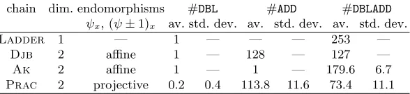
Operation Counts. Table 1 profiles the number of high-level operations required by each of our addition chain implementations on E. We used the decomposition in Theorem 1 to guarantee positive constant-bitlength multiscalars. In situations where side-channel resistance is not a priority, and theAk orPrac chain is preferable, variable-length decompositions could be used:
these would give lower operation counts and slightly faster average timings.
Table 1. Pseudo-group operation counts per scalar multiplication on thex-line for the 2-dimensional
Djb,Akand Prac chains (using endomorphism decompositions) and the 1-dimensional Ladder. The
counts forLadderandDjbare exact; those forPracandAkare averages, with corresponding standard
deviations, over 106 random trials (random scalars and points). In addition to the operations listed here, each chain requires a finalFp2-inversion to convert the result into affine form.
chain dim. endomorphisms #DBL #ADD #DBLADD
ψx, (ψ±1)x av. std. dev. av. std. dev. av. std. dev.
Ladder 1 — 1 — — — 253 —
Djb 2 affine 1 — 128 — 127 —
Ak 2 affine 1 — 1 — 179.6 6.7 Prac 2 projective 0.2 0.4 113.8 11.6 73.4 11.1
TheLadder andDjb chains offer some slightly faster high-level operations. In these chains,
the “difference elements” fed into the ADDs are fixed; if these points are affine, then this saves oneFp2-multiplication for eachADD. InLadder, the difference is always the affinex(P), so these savings come for free. In Djb, the difference is always one of the four values x(P), ψx(x(P)),
or (ψ±1)x(x(P)), so a shared inversion is used to convert ψx(x(P)) and (ψ±1)x(x(P)) from
projective to affine coordinates. While this costs oneFp2-inversion and six-Fp2 multiplications, it saves 253Fp2-inversions inside the loop.
6
Timings
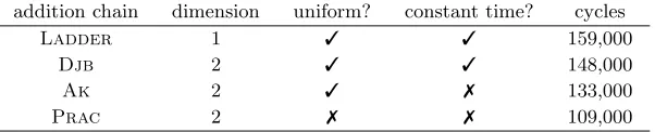
Table 2 lists cycle counts for our implementations run on an Intel Core i7-3520M (Ivy Bridge) processor at 2893.484 MHz with hyper-threading turned off, over-clocking (“turbo-boost”) disabled, and all-but-one of the cores switched off in BIOS. The implementations were compiled with gcc 4.6.3 with the-O2flag set and tested on a 64-bit Linux environment. Cycles were counted using the SUPERCOP toolkit [9].
The most meaningful comparison that we can draw is with Bernstein’s Curve25519software. Like our software,Curve25519works entirely on thex-line, from start to finish; using the uniform one-dimensional Montgomery ladder, it runs in constant time. Thus, fair performance comparisons can only be made between his implementation and the two of ours that are also both uniform and constant-time:Ladder and Djb. Benchmarked on our hardware with all settings as above,
Curve25519scalar multiplications ran in 182,000 cycles on average. Looking at Table 2, we see that using the one-dimensionalLadderon thex-line ofEgives a factor 1.14 speed up overCurve25519, 13It would be interesting to implement our techniques with Bernstein’s non-uniform two-dimensional
extended-gcd differential addition chain [4], which can outperformPrac (though it “takes more time
Table 2. Performance timings for four different implementations of compact, x-coordinate-only scalar multiplications targeting the 128-bit security level. Timings are given for the one-dimensional Montgomery
Ladder, as well as the two-dimensional chains (Djb,AkandPrac) that benefit from the application of
an endomorphism and subsequent short scalar decompositions.
addition chain dimension uniform? constant time? cycles
Ladder 1 ✓ ✓ 159,000
Djb 2 ✓ ✓ 148,000
Ak 2 ✓ ✗ 133,000
Prac 2 ✗ ✗ 109,000
while combining an endomorphism with the two-dimensionalDjbchain on thex-line ofE gives a
factor 1.23 speed up overCurve25519.
While there are several other implementations targeting the 128-bit security level that give faster performance numbers than ours, we reiterate that our aim was to push the boundary in the arena ofx-coordinate-only implementations.
Hamburg [19] has also documented a fast software implementation employingx-coordinate-only Montgomery arithmetic. However, it is difficult to compare Hamburg’s software with ours: his is not available to be benchmarked, and his figures were obtained on the Sandy Bridge architecture (and manually scaled back to compensate for turbo-boost being enabled). Nevertheless, Hamburg’s own comparison with Curve25519 suggests that a fair comparison between our constant-time implementations and his would be close.
Acknowledgements We thank Joppe W. Bos for independently benchmarking our code on his computer. The second author acknowledges that the notes of Appendix A grew from discussions with Joppe W. Bos on an earlier work [11].
References
1. Azarderakhsh, R., Karabina, K.: A new double point multiplication algorithm and its application to binary elliptic curves with endomorphisms. IEEE Trans. Comput. 99(PrePrints), 1 (2013)
2. Babai, L.: On Lov´asz’ lattice reduction and the nearest lattice point problem. Combinatorica 6(1), 1–13 (1986)
3. Bernstein, D.J.: Curve25519: New Diffie-Hellman speed records. In: Yung, M., Dodis, Y., Kiayias, A., Malkin, T. (eds.) Public Key Cryptography. LNCS, vol. 3958, pp. 207–228. Springer (2006)
4. Bernstein, D.J.: Differential addition chains (Feb 2006),http://cr.yp.to/papers.html#diffchain 5. Bernstein, D.J., Chuengsatiansup, C., Lange, T., Schwabe, P.: Kummer strikes back: new DH
speed records. Cryptology ePrint Archive, Report 2014/134 (version 20140224:033209) (2014), http://eprint.iacr.org/
6. Bernstein, D.J., Hamburg, M., Krasnova, A., Lange, T.: Elligator: elliptic-curve points indistinguish-able from uniform random strings. In: Sadeghi, A.R., Gligor, V.D., Yung, M. (eds.) ACM Conference on Computer and Communications Security. pp. 967–980. ACM (2013)
7. Bernstein, D.J., Lange, T.: Explicit-formulas database (accessed 10 October, 2013), http://www.hyperelliptic.org/EFD/
8. Bernstein, D.J., Lange, T.: SafeCurves: choosing safe curves for elliptic-curve cryptography (accessed 16 October, 2013),http://safecurves.cr.yp.to
9. Bernstein, D.J., Lange, T.: eBACS: ECRYPT Benchmarking of Cryptographic Systems (accessed 28 September, 2013),http://bench.cr.yp.to
10. Bernstein, D.J., Lange, T., Schwabe, P.: On the correct use of the negation map in the Pollard rho method. In: Catalano, D., Fazio, N., Gennaro, R., Nicolosi, A. (eds.) Public Key Cryptography. LNCS, vol. 6571, pp. 128–146. Springer (2011)
11. Bos, J.W., Costello, C., Hisil, H., Lauter, K.: Fast cryptography in genus 2. In: Johansson, T., Nguyen, P.Q. (eds.) EUROCRYPT. LNCS, vol. 7881, pp. 194–210. Springer Berlin Heidelberg (2013)
13. Fouque, P.A., Lercier, R., R´eal, D., Valette, F.: Fault attack on elliptic curve Montgomery ladder implementation. In: Breveglieri, L., Gueron, S., Koren, I., Naccache, D., Seifert, J.P. (eds.) FDTC. pp. 92–98. IEEE Computer Society (2008)
14. Frey, G., M¨uller, M., R¨uck, H.G.: The Tate pairing and the discrete logarithm applied to elliptic curve cryptosystems. IEEE Trans. Inform. Theory 45(5), 1717–1719 (1999)
15. Galbraith, S.D., Lin, X., Scott, M.: Endomorphisms for faster elliptic curve cryptography on a large class of curves. J. Cryptology 24(3), 446–469 (2011)
16. Gallant, R.P., Lambert, R.J., Vanstone, S.A.: Faster point multiplication on elliptic curves with efficient endomorphisms. In: Kilian, J. (ed.) CRYPTO. LNCS, vol. 2139, pp. 190–200. Springer (2001) 17. Gaudry, P.: Index calculus for abelian varieties of small dimension and the elliptic curve discrete
logarithm problem. J. Symb. Comp. 44(12), 1690–1702 (2009)
18. Gaudry, P., Hess, F., Smart, N.P.: Constructive and destructive facets of Weil descent on elliptic curves. J. Cryptology 15(1), 19–46 (2002)
19. Hamburg, M.: Fast and compact elliptic-curve cryptography. Cryptology ePrint Archive, Report 2012/309 (2012),http://eprint.iacr.org/
20. Kaib, M.: The Gauß lattice basis reduction algorithm succeeds with any norm. In: Budach, L. (ed.) FCT. LNCS, vol. 529, pp. 275–286. Springer (1991)
21. Koblitz, N.: CM-curves with good cryptographic properties. In: Feigenbaum, J. (ed.) CRYPTO. LNCS, vol. 576, pp. 279–287. Springer (1991)
22. Lochter, M., Merkle, J.: Elliptic curve cryptography (ECC) Brainpool standard curves and curve generation. RFC 5639 (2010),http://www.rfc-editor.org/rfc/rfc5639.txt
23. Menezes, A., Okamoto, T., Vanstone, S.A.: Reducing elliptic curve logarithms to logarithms in a finite field. IEEE Trans. Inform. Theory 39(5), 1639–1646 (1993)
24. Montgomery, P.L.: Speeding the Pollard and elliptic curve methods of factorization. Math. Comp. 48(177), 243–264 (1987)
25. Montgomery, P.L.: Evaluating recurrences of formXm+n=f(Xm, Xn, Xm−n) via Lucas chains (1992),
available atftp.cwi.nl:/pub/pmontgom/lucas.ps.gz
26. Pohlig, S.C., Hellman, M.E.: An improved algorithm for computing logarithms over GF(p) and its cryptographic significance. IEEE Trans. Inform. Theory 24(1), 106–110 (1978)
27. Pollard, J.M.: Monte Carlo methods for index computation (mod p). Math. Comp. 32(143), 918–924 (1978)
28. Satoh, T., Araki, K.: Fermat quotients and the polynomial time discrete log algorithm for anomalous elliptic curves. Comment. Math. Univ. St. Pauli 47(1), 81–92 (1998)
29. Schoof, R.: Counting points on elliptic curves over finite fields. J. Th´eor. Nombres Bordeaux 7(1), 219–254 (1995)
30. Semaev, I.: Evaluation of discrete logarithms in a group of p-torsion points of an elliptic curve in characteristicp. Math. Comp. 67(221), 353–356 (1998)
31. Smart, N.P.: The discrete logarithm problem on elliptic curves of trace one. J. Cryptology 12(3), 193–196 (1999)
32. Smart, N.P.: How secure are elliptic curves over composite extension fields? In: Pfitzmann, B. (ed.) EUROCRYPT. LNCS, vol. 2045, pp. 30–39. Springer (2001)
33. Smith, B.: Families of fast elliptic curves fromQ-curves. In: Sako, K., Sarkar, P. (eds.) ASIACRYPT. LNCS, vol. 8269, pp. 61–78. Springer (2013)
34. Solinas, J.A.: An improved algorithm for arithmetic on a family of elliptic curves. In: Kaliski, Jr., B.S. (ed.) CRYPTO. LNCS, vol. 1294, pp. 357–371. Springer (1997)
35. Stam, M.: Speeding up subgroup cryptosystems. Ph.D. thesis, Technische Universiteit Eindhoven (2003)
36. Straus, E.G.: Addition chains of vectors. Amer. Math. Monthly 71, 806–808 (1964)
37. Wiener, M.J., Zuccherato, R.J.: Faster attacks on elliptic curve cryptosystems. In: Tavares, S.E., Meijer, H. (eds.) Selected Areas in Cryptography. LNCS, vol. 1556, pp. 190–200. Springer (1998)
A
Efficient Arithmetic in
F
pand
F
p2We access lower level integer arithmetic for efficient addition, subtraction, multiplication and squaring operations in Fp and Fp2 where p = 2127−1, see §2. At this level, elements of Fp are
Semi-reduced values can be used in any chain of operations without causing an exception, since all of our algorithms are designed to accept inputs and produce outputs in the interval [0, p]. The implementor should reduce each output into the range [0, p) at the very end of the target computation, in order to satisfy unique representation field elements. This type of arithmetic has already been exploited in earlier works, such as [11], but a thorough exposition has not yet appeared.
We will be frequently referring back to the divisibility lemma of integers.
Lemma 1. Let u, v∈Z with v >0. Then there exist uniqueq, r∈Z such that u=r+qv and
0≤r < v. In particular, q=⌊u/v⌋andr=u− ⌊u/v⌋v where ⌊.⌋is the floor function.
In what follows, the “mod 2128” and “mod 2256” operators, are included (even though they are often unnecessary) to reinforce the fact that all arithmetic operations are being performed on an unsigned integer arithmetic circuit over a 128-bit data type. We letki denote theithsignificant bit
of an integerkand use (ki, . . . , kj) to denote the integer formed by the bit-string that starts with
ki, continues with bits in order of increasing significance, and ends withkj (with 0≤i≤j≤127).
Although it is possible to provide much shorter arguments for sections A.1-5, we prefer to keep the notes in longer format in order to assist easier verification.
It should be noted that all of the techniques in this section avoid branching. This is highly desirable for an efficient implementation, especially on an architecture with pipelining capability.
A.1 Semi-reduced Addition modulop
The operation (a+b) modpis replaced by Algorithm 1.
Input:a, b∈Zsuch that 0≤a, b≤p.
Output:f∈Zsuch thatf≡(a+b) (modp) and 0≤f≤p.
c:= (a+b) mod 2128; 1
d:= (c0, c1, . . . , c126),e:= (c127); 2
f:= (d+e) mod 2128 ;
3
returnf;
4
Algorithm 1: Semi-reduced addition modulop
– Line-1:Notice that 0≤c=a+b≤2p <2128.
– Line-2:Use Lemma 1 to writec =d+ 2127efor integers 0≤d <2127 and e. There are two cases to investigate:
• Case 1: Assume thata+b≤p. The bounds onc anddimply that
0/2127
≤
c/2127
=
(d+ 2127e)/2127
=
d/2127
+
2127e/2127
= e ≤
p/2127
, so e = 0. Thus a+b ≡
d+ 2127e≡d+ 2127·0≡d+ 0≡d+e (mod p).
• Case 2: Assume that a+b > p. Then p < c ≤2p. The bounds on c and d imply that
(p+ 1)/2127
≤ e ≤
2p/2127
, soe = 1. The bounds on c also imply that p−2127 < c−2127 ≤2p−2127 and we have d=c−2127e =c−2127, so 0 ≤d < p. Thusa+b ≡ d+ 2127e≡d+ 2127·1≡d+ 1≡d+e (mod p).
– Line-3:A semi-reduced output is given byf := (d+e) mod 2128, observing that 0≤f ≤p.
A.2 Semi-reduced Subtraction modulop
Input:a, b∈Zsuch that 0≤a, b≤p.
Output:f∈Zsuch thatf≡(a−b) (modp) and 0≤f≤p.
c:= (a−b) mod 2128 ;
1
d:= (c0, c1, . . . , c126),e:= (c127); 2
f:= (d−e) mod 2128 ;
3
returnf;
4
Algorithm 2: Semi-reduced subtraction modulop
– Line-2:Use Lemma 1 to writec =d+ 2127efor integers 0≤d <2127 and e. There are two cases to investigate:
• Case 1: Assume that a ≥ b. Then 0 ≤ c = a−b ≤ p. The bounds on c and d imply that
0/2127
≤
c/2127
=
(d+ 2127e)/2127
= e≤
p/2127
, so e = 0. Thus a−b ≡
d+ 2127e≡d−e (mod p).
• Case 2: Assume thata < b. Thenc= 2128+a−band−p≤a−b <0. So, 2127< c <2128. The bounds on c and d imply that
(2127+ 1)/2127
≤e≤
(2128−1)/2127
, so e = 1. The bounds on c also imply that 2127 −2127 < c−2127 < 2128−2127, and we have d=c−2127e=c−2127. So, 0< d≤pand d≥e. Thusa−b≡(2128+a−b)−2128≡ c−2128≡d+ 2127e−2128≡d−e (modp).
Line-3:A semi-reduced output is given byf := (d−e) mod 2128, observing that 0≤f ≤p.
A.3 Semi-reduced Multiplication modulop
The operation (ab) modpis replaced by Algorithm 3.
Input:a, b∈Zsuch that 0≤a, b≤p.
Output:f∈Zsuch thatf≡(ab) (modp) and 0≤f≤p.
c:= (ab) mod 2256 ;
1
d:= (c0, c1, . . . , c126),e:= (c127, c128, . . . , c253); 2
f:= semi-add(d, e);
3
returnf;
4
Algorithm 3: Semi-reduced multiplication modulop
– Line-1:Notice that 0≤c=ab≤p2<2256.
– Line-2:Use Lemma 1 to writec=d+ 2127efor integers 0≤d <2127 ande. The bounds on c anddimply that
0/2127
≤
c/2127
=
(d+ 2127e)/2127
=e≤
p2/2127
, so 0≤e < p. – Line-3:Noting thatab≡d+ 2127e≡d+ (2127−1)e+e≡d+pe+e≡d+e (mod p), that
0 ≤ d, e ≤ p, and that 0 ≤ d+e ≤ 2p, a semi-reduced output is obtained by Algorithm 1 applied on the operandsdande.
A.4 Lazy Semi-reduction modulo pfollowing a Double-Word Addition
The lazy reduction (aˆb+ ˆab) modpis replaced by Algorithm 4. – Line-1:Notice that 0≤c=aˆb+ ˆab≤2p2<2256.
Input:a,ˆa, b,ˆb∈Zsuch that 0≤a,ˆa, b,ˆb≤p.
Output:h∈Zsuch thath≡(abˆ+ ˆab) (modp) and 0≤h≤p.
c:= (aˆb+ ˆab) mod 2256 ;
1
d:= (c0, c1, . . . , c126),e:= (c127, c128, . . . , c253),f:= (c254); 2
g:= (e+f) mod 2128 ;
3
h:= semi-add(d, g);
4
returnh;
5
Algorithm 4: Lazy semi-reduction modulopfollowing a double-word addition
• Case 1: Assume that aˆb+ ˆab < (p+ 1)2. Then 0 ≤ c < (p+ 1)2. The bounds on c, d, and e imply that
0/(2127)2
≤
c/(2127)2
=
(d+ 2127e+ (2127)2f)/(2127)2
= f ≤
((p+ 1)2−1)/(2127)2
, sof = 0. Thusaˆb+ˆab≡d+2127(e+2127f)≡d+2127(e+2127·0)≡ d+ 2127(e+ 0)≡d+ 2127(e+f) (modp) and 0≤e+f < p.
• Case 2: Assume that aˆb+ ˆab ≥ (p+ 1)2. Then (p+ 1)2 ≤ c ≤ 2p2. The bounds on c, d, and e imply that
(p+ 1)2/(2127)2
≤f ≤
2p2/(2127)2
, so f = 1. The bounds on c also imply that (p+ 1)2−(2127)2≤c−(2127)2≤2p2−(2127)2, and we haved+ 2127e= c−(2127)2f =c−(2127)2. So, 0≤d+ 2127e≤((p−1)2−2). The bounds on d+ 2127e imply that
0/2127
≤
(d+ 2127e)/2127 ≤
((p−1)2−2)/2127
, so 0≤e <(p−2). Thus aˆb+ ˆab≡d+ 2127(e+ 2127f)≡d+ 2127(e+ 2127·1)≡d+ 2127(e+ 1)≡d+ 2127(e+f) (modp) and 0≤e+f < p.
– Line-3:Setg:= (e+f) mod 2128where 0≤g≤p.
– Line-4: Noting that d+ 2127(e+ 2127f) ≡ d+ 2127g ≡ d+g (modp), that 0 ≤ d, g ≤ p, and that 0 ≤d+g ≤2p, a semi-reduced output is obtained by Algorithm 1 applied on the operandsdandg.
A.5 Lazy Semi-reduction modulop following a Double-Word Subtraction
The lazy reduction (ab−ˆaˆb) modpis replaced by Algorithm 5.
Input:a,ˆa, b,ˆb∈Zsuch that 0≤a,ˆa, b,ˆb≤p.
Output:h∈Zsuch thath≡(ab−ˆaˆb) (modp) and 0≤h≤p.
c:= (ab−ˆaˆb) mod 2256 ;
1
d:= (c0, c1, . . . , c126),e:= (c127, c128, . . . , c253),f:= (c254),g:= (c255); 2
h:= (e−f) mod 2128 ;
3
j:= semi-add(d, g);
4
returnj;
5
Algorithm 5: Lazy semi-reduction modulopfollowing a double-word subtraction
– Line-1:Notice that 0≤c <2256.
– Line-2: Use Lemma 1 to write c =d+ 2127(e+ 2127(f + 2g)) for integers 0 ≤d, e < 2127, 0≤f <2, andg. There are two cases to investigate:
• Case 1: Assume that ab ≥ ˆaˆb. Then 0 ≤ c = ab −ˆaˆb ≤ p2. The bounds on c, d, e and f imply that
0/(2127)2
≤
c/(2127)2
=
(d+ 2127e+ (2127)2(f + 2g))/(2127)2
= f+ 2g≤
p2/(2127)2
; that isf+ 2g= 0. So,f =g= 0. Thusd+ 2127(e+ 2127(f+ 2g))≡ d+ 2127(e+ 2127·0)≡d+ 2127(e−0)≡d+ 2127(e−f) (modp).
(2256−p2)/(2127)2
≤ f + 2g ≤
(2256−1)/(2127)2
, so f + 2g = 3 and f = g = 1. The bounds onc also imply that 2256−p2−3(2127)2= 2128−1≤c−3(2127)2<2256− 3(2127)2 and we also have d+ 2127e=c−(2127)2(f+ 2g) =c−3(2127)2. So, 2128−1 ≤ d+ 2127e. The bounds on d+ 2127e imply that
(2128−1)/2127
≤
(d+ 2127e)/2127
<
(2256−3(2127)2)/2127
= 2127, so 1≤e <2127ande≥f. Thus
ab−ˆaˆb ≡(2256+ab−ˆaˆb)−2256 = c−2256 ≡ c−4
≡d+ 2127(e+ 2127(f+ 2g))−4
≡d+ 2127(e+ 2127(1 + 2·1))−4
≡d+ 2127(e−1) ≡ d+ 2127(e−f) (mod p). – Line-3:Seth:= (e−f) mod 2128where 0≤h≤p.
– Line-4:Noting thatd+ 2127(e+ 2127(f+ 2g))≡d+ 2127h≡d+h (modp), that 0≤d, h≤p, and that 0 ≤d+h≤2p, a semi-reduced output is obtained by Algorithm 1 applied on the operandsdandh.
A.6 Addition and Subtraction in Fp2
Leta,ˆa, b,ˆb∈Zand 0≤a,a, b,ˆ ˆb≤p. We use the obvious method which computes (a+ ˆai) + (b+ ˆbi) as ((a+b) modp) + ((ˆa+ ˆb) modp)i. Both modular additions are replaced by Algorithm 1. Analogous comments apply for the case of subtraction which uses Algorithm 2.
A.7 Multiplication inFp2
Let a,ˆa, b,ˆb ∈ Z and 0 ≤ a,ˆa, b,ˆb ≤ p. On the target architecture, we experienced the best performance for computing (a+ ˆai)(b+ ˆbi) by coupling a Karatsuba-based operation scheduling with two lazy reductions. This computes the product as
(ab−ˆaˆb) modp+
(a+ ˆa)(b+ ˆb)−ab−aˆˆb
modpi.
The routine starts with two integer additionst0 :=a+ ˆaand t1 :=b+ ˆb satisfying 0≤t0, t1 < (2128 −1). The routine continues with the 3 integer multiplications t
2 := t0t1, t3 := ab and t4 := ˆaˆb satisfying 0 ≤ t2 ≤ (2128−2)2 < 2256 and 0 ≤ t3, t4 ≤ (2127 −1)2 < 2254. Since t2 > t3 and (t2−t3) > t4, the integer value t5 := (t2−t3)−t4 is positive and satisfies both 0 ≤t5 ≤2p2 <2255 and t5 =aˆb+ ˆab. The reduction of t5 is performed as in Algorithm 4. The reduction oft6:= (t3−t4) mod 2256 is performed as in Algorithm 5.
A.8 Squaring inFp2
Leta,ˆa, b,ˆb∈Zand 0≤a,ˆa, b,ˆb≤p. On the target architecture, we experienced that a lazy semi-reduction strategy gives the same timings as the (non-lazy) semi-semi-reduction strategy for computing (a+ ˆai)2= (a−ˆa)(a+ ˆa)
+ 2aˆa
i.
A.9 Other Operations inFp2
Many other Fp2 operations can be efficiently performed by Fp arithmetic only. For instance, negation can be performed as −a = (0−a) + (0−aˆ)i, p-th powering as ap = a+ (0−aˆ)i,
and inversion asa−1=a(a2+ ˆa2)p−2+ (0−ˆa(a2+ ˆa2)p−2)i – our F
B
How was This Curve Chosen?
The curve-twist pair implemented in this paper was chosen from the family of degree-2Q-curve reductions with efficient endomorphisms (over Fp2) described in [33]. These curves are equipped with efficient endomorphisms, and the arithmetic properties of the family are not incompatible with twist-security.
We fixed p = 2127−1, a Mersenne prime; this p facilitates very fast modular arithmetic. Next, we chose a tiny nonsquare to defineFp2 =Fp(i) with i2=−1; this makes for slightly faster
Fp2-arithmetic, and much simpler formulæ. The most secure group orders for a Montgomery curve-twist pair (E,E′
) over Fp2 have the form (#E,#E′) = (4N,8N′) (or (8N,4N′)) with N and N′ prime. The cofactor of 4 is forced by the existence of a Montgomery model, and then p2 ≡ 1 (mod 8) forces a cofactor of 8 on the twist.
The family in [33,§5] is parametrised by a free parameters; each choice of s in Fp yields a
curve overFp2, each in a distinctFp-isomorphism class. If the curve corresponding to sin Fp has
a Montgomery model E : BY2 = X(X2+AX+ 1) overF
p2, then 8/A2 = 1 +si. If we write A=A0+A1iwithA0andA1 in Fp, then
A40+ 2A20A21+A41+ 8(A21−A20) = 0. (5) To optimise performance, we searched for parameter values s in Fp yielding Montgomery representations with “small” coefficients: that is, whereA0 andA1 could be represented as small integers. But in view of Eq. (5), for any small value ofA1 there are at most four corresponding possibilities forA0, none of which have any reason to be small (and vice versa). Given the number of curves to be searched to find a twist-secure pair, we could not expect to find a twist-secure curve with bothA0 andA1 small. OurFp2-arithmetic (described in Appendix A) placed no preference on which of these two coefficients should be small, so we flipped a coin and restricted our search to syielding A1 with integer representations less than 232 (occupying only one word on 32- and 64-bit platforms). The constant appearing in Montgomery’s formulæ [24, p. 261] is (A+ 2)/4, so we also required the integer representation ofA1to be congruent to 2 modulo 4.
Our search prioritisedA1values whose integer representations had low signed Hamming weight, in the hope that multiplication byA1 might be faster when computed via sequence of additions and shifts. We did not find any curve-twist pairs with optimal cofactors andA1of weight 1, 2, or 3, but we found ten such pairs with A1 of weight 4. Three of these pairs had anA1 of precisely 32 bits; the curve-twist pair in §2 corresponds to thesmallest suchA1. Although the low signed Hamming weight ofA1did not end up improving our implementation, the small size ofA1yielded a minor but noticeable speedup.
The takeaway message is that the construction in [33, §5] is flexible enough to find a vast number of twist-secure curves over any quadratic extension field, to which all of the techniques in this paper can be directly applied (or easily adapted), regardless of how the parameter search is designed. Such curve-twist pairs can be readily found in averifiably randommanner, following, for instance, the method described in [22,§5].
C
Bernstein’s Uniform Two-Dimensional Differential Addition Chain
Algorithm 6 is a concrete adaptation of Bernstein’s addition chain [4,§4] to our curveE, following the multiscalar decomposition described in §4. We use the usual formulæ (see [7]) for pseudo-doubling, pseudo-addition, and for the combination of the two, writing their inputs and outputs as follows. For pseudo-doubling, we write
x([2]R) =DBL(x(R)) ;
for pseudo-addition, we write