Finding Roots in
F
pnwith the Successive Resultants Algorithm
Christophe Petit ?
UCL Crypto Group
To appear in the LMS Journal of Computation and Mathematics, as a special issue for ANTS (Algorithmic Number Theory Symposium) conference.
Abstract. The problem of solving polynomial equations over finite fields has many ap-plications in cryptography and coding theory. In this paper, we consider polynomial equa-tions over a “large” finite field with a “small” characteristic. We introduce a new algorithm for solving this type of equations, called the Successive Resultants Algorithm (SRA) in the sequel. SRA is radically different from previous algorithms for this problem, yet it is conceptually simple. A straightforward implementation using Magma was able to beat the built-in functionRoots for some parameters. These preliminary results encourage a more detailed study of SRA and its applications. Moreover, we point out that an extension of SRA to the multivariate case would have an important impact on the practical security of the elliptic curve discrete logarithm problem in small characteristic.
1 Introduction
Letp be a “small” prime number and let dand nbe two natural numbers. Let Fpn be the finite field with pn elements, and let f be a polynomial of degree d over Fpn. The
root-finding problem is the problem of computing one, several or all elements x ∈Fpn such that
f(x) = 0.
This problem has a lot of applications, in particular for the more general problem of factoring f and its applications [19], but also in cryptography and in coding theory.
Many algorithms have been proposed to solve this problem. Most of them first reduce
f to a square-free and split polynomial, and then progressively factor this polynomial through successive attempts [1,13,17,4].
In this paper, we introduce the Successive Resultant Algorithm (SRA), a new de-terministic algorithm to solve this problem. Our approach is conceptually simple, yet radically different from previous ones. We show that SRA has an asymptotic complex-ity comparable to Berlekamp’s well-known trace algorithm for large degree polynomials (d2 > n or d > n depending on the type of polynomial arithmetic) and in all cases if certain field constants used in the algorithm are precomputed. We also provide a straightforward implementation using Magma [21] and we emphasize some parameter ?Supported by an F.R.S.-FNRS postdoctoral research fellowship at Universit´e catholique de Louvain,
sets for which this implementation has beaten Magma’s corresponding built-in function
Roots.
We finally discuss open problems and a potential extension of our work. In particular, we believe that our ideas form an important step towards a much more efficient resolu-tion of polynomial systems arising from a Weil descent in the multivariate case [11]. We stress that a multivariate version of SRA would have a very strong impact on the practi-cal security of the Elliptic Curve Discrete Logarithm Problem in the small characteristic case.
1.1 Outline
This paper is organized as follows. In Section 2, we review the basics of finite field arithmetic and previous root finding algorithms inFpn. In Sections 3 and 4, we provide both a basic version of our algorithm and an optimized version for fast arithmetic. We also analyze the complexity of our algorithms in these sections. In Section 5, we provide experimental timings obtained with a Magma implementation of our algorithm. We finally conclude the paper and present interesting open problems in Section 6.
2 Preliminaries
2.1 Finite Field and Polynomial Ring Arithmetic
Letp be a “small” prime number, let nbe a positive integer, letFpn be the finite field with pn elements and let f be a univariate polynomial of degree d over Fpn. We also definesas the number of solutions of f overFpn.
We will suppose that p is small enough for us to treat it as a constant in our estimations. Unless explicitely mentioned, we take an operation overFp as a basic step
in all our complexity evaluations. We use both the “big O” and “big O tilde” notations in our estimations. Remember that f is ˜O(g) if and only if f is O(glogc(g)) for some constant c. Solving a linear system of size m over Fp has a cost O(mω), where ω is
the linear algebra constant. The best algorithms today achieveω as small as 2.3727 for generic systems [22].
We denote bya(n) and m(n) the cost of an addition and a multiplication over Fpn, and byA(d) andM(d) the cost of an addition and a multiplication of two polynomials of degreedoverFpn. We also denote byG(d) the cost of computing the greatest common divisor of two polynomials of degree dover Fpn. We will consider both “classical” and “fast” polynomial arithmetics in this paper.
Classical arithmetic is a reasonable choice today for small and medium parameter sizes for which the overhead of fast arithmetic algorithms is significant. Using this type of arithmetic, field additions and polynomial additions are respectively executed inO(n) and O(dn). Polynomial multiplications are performed in a straightforward way with a quadratic cost with respect to the degree. As a result, we have m(n) = O(n2) and M(d) =O(d2n2).
Multiplications modulo a polynomial of degree d can be performed at essentially the same cost. Field additions and polynomial additions are executed inO(n) andO(dn) as before. Fast arithmetic is available today in the computer algebra system Magma [21]. The greatest common divisor (gcd) of two polynomials of degreedcan be computed inO(d2) field operations using the Euclidean algorithm or ˜O(d) field operations using a more involved Sch¨onhage-type algorithm [14,16]. In our estimations, we will assume for simplicity that the Euclidean algorithm is always used together with classical arithmetic and that fast gcd algorithms are always used together with fast arithmetic. Table 1 summarizes the various costs respectively for “classical” and “fast” arithmetics with this convention.
Table 1: Costs of finite field and polynomial arithmetic
a(n) m(n) A(d) M(d) G(d) ClassicalO(n)O(n2)O(dn)O(d2n2)O(d2n2)
Fast O(n) ˜O(n) O(dn) O˜(dn) O˜(dn)
2.2 Finding Roots in Fpn
Let f be a univariate polynomial over Fpn with degree d having exactly s distinct roots. The problems of computing one, several or all roots off have many applications in cryptography and coding theory. Several algorithms have been proposed for this problem, with complexities depending on the arithmetic type and on the parameters d
and n.
In most root-finding algorithms, the polynomialf is assumed to be split and square-free (all its irreducible factors are linear and distinct), hence s=d. Given an arbitrary polynomial f, its squarefree split part is easily recovered through the gcd computa-tion gcd(xpn−x, f(x)), after successively computing the polynomials xpi modf(x) for
i = 0, . . . , n −1 with a square-and-multiply algorithm. These computations require
O(d2n) operations over Fnp or O(d2n3) operations over Fp using standard arithmetic,
and only ˜O(dn2) over Fp using fast arithmetic.
The simplest algorithms for the root finding problem are variants of exhaustive search. A better approach was proposed by Berlekamp et al. in [3]. This algorithm first constructs a polynomial L such that L(x) = Pd−1
i=0 Lixp
i
and f divides L. The computation of L only requires computing xpi modf(x) for i= 0, . . . , d−1 and then solving a d×d linear system over Fpn. Since L is a linear application over Fp, the algorithm of [3] then solvesLwith linear algebra over Fp and tests each solution forf.
The algorithm is still not very efficient in general since L may have up to pd solutions in the worst case, and all these solutions are tested to identify the roots off.
as
f(x) = Y
r∈Fp
gcd f(x),Tr(αix)−r
for some α∈ Fpn with algebraic degree n and for various i∈ {0, . . . , n−1}. Each gcd computation costs O(d2n3) or ˜O(dn2) operations over Fp, using respectively classical
or fast arithmetics. It is known that at least one value of i leads to a non-trivial fac-torization [1] and that testing O(logn) of them is required on average [10]. Once f is split into at least two distinct factors, the process is then recursively applied to all these factors. Since the recursive step has a cost larger than any linear function ind, we can in fact recover all the linear factors of f using O(d2n3) or ˜O(dn2) operations over
Fp,
depending on the arithmetic type [18, Th. 14.11].
Other splitting strategies are also possible. When p is odd, Rabin’s root-finding algorithm [13] computes gcd f(x),(x+δ)(pn−1)/2−1for a randomδ ∈Fpn. The total complexity of this approach is similar to BTA.
Compared to BTA, the Affine Method of van Oorschot and Vanstone [17] first com-putes a polynomialL as in [3]. The trace function used in BTA is generalized to other polynomialsB(x) that are also linear over Fp. The gcd between f and B is then
com-puted in two steps as gcd(f(x),gcd(L(x), B(x)). The affine method is more efficient than BTA whend < n and standard arithmetic is used, since their respective costs are then equivalent to O(d2n) and O(dn2) multiplications over
Fpn [17]. However with fast arithmetic, the computationB(x) modL(x) alone already requires ˜O(dn2) following the method of [17], so the Affine Method is at best as fast as BTA.
The modular Frobenius exponentiation x → xpi modf(x) is a key ingredient of all the methods described above. Von zur Gathen and Shoup [20] suggested to use repeated modular compositions and multipoint evaluation instead of the straightfor-ward square and multiply algorithm to perform these exponentiations. This idea led to the asymptotically fastest polynomial factorization algorithms today. Kaltofen and Shoup [8] proposed an algorithm running in a time ˜O(d1.815n2), though not completely
practical since it relies on fast matrix multiplication. By introducing new, asymptoti-cally faster algorithms for the modular composition problem, Kedlaya and Umans [9] derived a randomized algorithm to factorf entirely in time ˜O(d3/2n+dn2).
Our new algorithm has an asymptotic complexityO(n4+d2n3) with standard arith-metic and ˜O(n3+dn2) with fast arithmetic, where the n4 and n3 terms are spent on computing certain field constants. This asymptotic complexity is similar to BTA for large degree polynomials or if the field constants are precomputed. Our experiments suggest that the new algorithm may compete with the ones currently used in practice for some parameters.
3 The Successive Resultants Algorithm
3.1 A polynomial system
Let {v1, . . . , vn} be an arbitrary basis of Fpn over Fp. From this basis, we recursively definen+ 1 functionsL0, L1, . . . , Ln from Fpn toFpn such that
L0(z) =z
L1(z) = Q
i∈FpL0(z−iv1)
L2(z) =Qi∈FpL1(z−iv2)
. . .
Ln(z) =Qi∈FpLn−1(z−ivn).
The functions Lj are examples oflinearized polynomials as defined in [2, Ch. 11]. They
satisfy the following properties.
Lemma 1. a) Each polynomial Li is split and its roots are all elements of the vector space generated by {v1, . . . , vi}. In particular, we have Ln(z) =zp
n
−z. b) We have Li(z) =Li−1(z)p−aiLi−1(z) where ai := (Li−1(vi))p−1.
c) If we identify Fpn with the vector space (Fp)n, then each Li is a p to 1 linear map
of Li−1(z) and a pi to 1 linear map of z.
Proof. Part a) is clear by construction. We first prove Part b) forL1. We havezp−z= Q
i∈Fp(z−i) by identification of the roots on both sides. Substituting x by z/v1, we deduce zp−vp−1
1 z = Q
i∈Fp(z−iv1) =L1(z). From this equality, it is clear that L1 is a linear map over Fp, and in particular L1(z−iv2) = L1(z)−iL1(v2) for all i ∈ Fp.
Substituting z by Lj(z) andv1 by Lj(vj+1), part b) follows by induction. For part c),
notice that the kernel of the linear map z→Q
i∈Fp(z−i) has sizep. We now consider the following polynomial system:
f(x1) = 0
xpj −ajxj =xj+1 j= 1, . . . , n−1
xpn−anxn= 0
(1)
where theai ∈Fpn are defined as in Lemma 1. Any solution of this system provides us with a root off by the first equation, and the nlast equations together imply that this root belongs to Fpn.
Lemma 2. Let (x1, x2, . . . , xn)be a solution of System (1). Thenx1∈Fpn is a solution
of f. Conversely, given a solution x1 ∈ Fpn of f, we can reconstruct a solution of
System (1) by setting x2 =xp1−a1x1, etc.
Proof. By Lemma 1, the equations of System (1) implyxi=Li−1(x1), and in particular
xpn−anxn=xp
n
3.2 Solving System (1) with Resultants
In order to solve System (1), we notice that it has a quasi-diagonal structure: the first equation only depends on x1, each equation xpj −ajxj =xj+1 only depends on xj and
xj+1, and the last equation only depends on xn. Our new algorithm will exploit this
structure to solve System (1), hence the polynomialf.
In the first step of the algorithm, we successively compute f(1) = f, f(2), . . . , f(n)
such thatf(j) has the same degree as f and only depends on the variable xj. Letfi be
the coefficients off, such that f(x) =Pd
i=0fixi. We compute f(2) as
f(2)(x2) = Resx1(f
(1)(x
1), x2−(xp1−a1x1))
=
1 0 . . . 0 −a1 −x2 0 0 . . . 0
1 0 . . . 0 −a1 −x2 0 0 . . . 0
. . .
. . .
1 0 . . . 0 −a1−x2 0
1 0 . . . 0 −a1 −x2
fdfd−1 fd−2 . . . fp+1 fp fp−1 . . . f2 f1 f0 0 . . . 0 0
fd fd−1fd−2 . . . fp+1 fp fp−1 . . . f2 f1 f0 0 . . . 0
. . .
fd fd−1fd−2 . . . fp+1 fp fp−1 . . . f2 f1 f0 0
fd fd−1 fd−2 . . . fp+1 fp fp−1. . . f2 f1 f0
, (2)
which is clearly a polynomial in x2 only. Its degree is exactly d since the variable x2
appears exactly d times in the above determinant, in different rows and columns. We then successively compute
f(j+1)(xj+1) = Resxj
f(j)(xj), xj+1−(xpj −ajxj)
forj = 2, . . . , n−1, which all have degreed for the same reasons. A simple algorithm to compute these resultants is provided in Section 3.4 below.
In the second step of our algorithm, we successively recover values forxn, xn−1, . . .,
and finallyx1. We first compute
g(n)(xn) := gcd
f(n)(xn), xpn−anxn
.
By construction, g(n) is a polynomial of degree at most p, dividing xpn−anxn. If this
polynomial is a non zero constant, thenf has no solution overFpn. Otherwise, it follows from Lemma 1 c) thatg(n)is split. Its roots ˆxncorrespond to the values of the variable
xn in the solutions of System (1). For each of these ˆxn values, we then compute
g(n−1)(xn−1) := gcd
f(n−1)(xn−1),xˆn−(xpn−1−an−1xn−1)
. (3)
By construction, g(n−1) is a polynomial of degree at most p, dividing ˆxn−(xpn−1 −
an−1xn−1). If this polynomial is a constant, then there is no solution. Otherwise, it
follows from Lemma 1 c) that g(n−1) is split. We compute the factorization of g(n−1)
the linear polynomial ˆxn−(xpn−1−an−1xn−1) followed by a small exhaustive search.
The roots of g(n−1) correspond to the values of the variables xn−1 in the solutions
of System (1). Proceeding recursively, we finally obtain all x1 values that satisfy the
equationf(1)(x1) = 0. The whole algorithm is deterministic if no probablistic algorithm
is used for the resultant computation and small degree root-finding routines.
3.3 Example
We provide a small example of SRA execution when p= 2, n= 5 and d= 6. Letα be a root of t5+t2+ 1 over F25. Let vi:= αi−1,i= 1, . . . ,5. The precomputation step of SRA leads to a1 = 1,a2 =α19,a3=α6,a4=α4 and a5 =α2.
Let now f(x) :=x5+α20x4+α27x3+α4x2+α14x+α9. In the first step of SRA, we successively compute
f(1)(x1) =x51+α20x41+α27x31+α4x21+α14x1+α9,
f(2)(x2) =x52+α28x42+α23x32+α4x22+α12x2+α19,
f(3)(x3) =x53+αx43+α23x33+α23x23+x3,
f(4)(x4) =x54+α4x44+α7x34+α11x24,
f(5)(x5) =x55+αx35.
In the second step of SRA, we then compute
g(5)(x5) = gcd(f(5)(x5), x25+a5x5) =x5,
g(4)(x4) = gcd(f(5)(x5), x24+a4x4) =x24+α4x4=x4(x4+α4).
The root ˆx4=α4 leads to
g(3)(x3) = gcd(f(3)(x3),xˆ4+x23+a3x3) =x3+α3,
g(2)(x2) = gcd(f(2)(x2),xˆ3+x22+a2x2) =x2+α,
g(1)(x1) = gcd(f(1)(x1),xˆ2+x21+a1x1) =x1+α3.
The root ˆx4= 0 leads to
g(3)(x3) = gcd(f(3)(x3),xˆ4+x23+a3x3) =x23+α6x3 =x3(x3+α6).
The root ˆx3= 0 leads to
g(2)(x2) = gcd(f(2)(x2),xˆ3+x22+a2x2) =x2+α19,
g(1)(x1) = gcd(f(1)(x1),xˆ2+x21+a1x1) =x1+α18.
The root ˆx3=α6 leads to
g(2)(x2) = gcd(f(2)(x2),xˆ3+x22+a2x2) =x2+α30,
g(1)(x1) = gcd(f(1)(x1),xˆ2+x21+a1x1) =x1+α19.
The solution set of f is therefore {α3, α18, α19}. For this example, the computation of this set required 5 resultants, 10 gcds and the factorizations of 2 degree 2 (linear over
3.4 Computing the Resultants
Resultants are the basic operations in the first step of SRA algorithm. Under simple row manipulations, we have
f(2)(x2) = Resx1(f
(1)(x
1), x2−(xp1−a1x1))
=
1 0. . . 0 −a1−x2 0 0 . . . 0
1 0 . . . 0 −a1−x20 0 . . . 0
. . . . . .
1 0 . . . 0 −a1 −x2 0
1 0 . . . 0 −a1 −x2
Fp−1,p−1 . . . Fp−1,2Fp−1,1Fp−1,0
Fp−2,p−1 . . . Fp−2,2Fp−2,1Fp−2,0
. . .
F1,p−1 . . . F1,2 F1,1 F1,0
F0,p−1 . . . F0,2 F0,1 F0,0
=
Fp−1,p−1 . . . Fp−1,2 Fp−1,1Fp−1,0
Fp−2,p−1 . . . Fp−2,2 Fp−2,1Fp−2,0
. . .
F1,p−1 . . . F1,2 F1,1 F1,0
F0,p−1 . . . F0,2 F0,1 F0,0
whereFj,i satisfy p−1 X
i=0
Fj,i(x2)xi1 =x j
1f(x1) mod (x2−(xp1−a1x1)).
In particular,pdegFj,i+i≤d+j. The resultant can therefore be computed as follows:
1. Reduce the last row of (2) by the first d ones to obtain the coefficients F0,i. This
amounts to computing
h(x1, x2) := p−1 X
i=0
F0,i(x2)xi1 =f(x1) mod (xp1−a1x1−x2). (4)
2. Shift these coefficients on the left and further reduce by the first drows to obtain all coefficients Fi,j. This amounts to successively computing
p−1 X
i=0
Fj,i(x2)xi1=x j
1h(x1, x2) mod (x1p−a1x1−x2)
=x1
xj−11 h(x1, x2)
mod (xp1−a1x1−x2)
=
p−1 X
i=1
Fj−1,i−1(x2)xi1+Fj−1,p−1(x2) (a1x1+x2)
3.5 Complexity Analysis
The complexity of SRA can be analyzed as follows. First, we note that all the valuesai
of Lemma 1 can be (pre)computed at a total cost ofO(n2) operations over
Fpn, that is
O(n4) operations over Fp using classical arithmetic or ˜O(n3) operations over Fp using
fast arithmetic.
Next we evaluate the cost of the resultant algorithm of Section 3.4. The last row can be computed withO(d) elementary row reduction steps, each one involving O(p·d
p) =
O(d) multiplications overFpn. All the other polynomialsFi,j can then be computed using
O(d) operations over Fpn. Finally, the last determinant requires O(p3) multiplications of polynomials of degrees at mostdover Fpn. Computing one resultant therefore costs
O(d2n2) operations over Fp using standard arithmetic and ˜O(d2n) operations over Fp
using fast arithmetic. Completing the first step of SRA costsnresultants, that isO(d2n3) operations overFp using standard arithmetic and ˜O(d2n2) operations overFp using fast
arithmetic.
In the second step of SRA, we compute several gcds between a degree d and a degree ppolynomial over Fpn. This requires O(d) operations overFpn for each gcd. We also need to factor all the polynomials g(j) that have degree larger than 1. Since each polynomial g(j) has degree at most p, each factorization costs O(n3) operations with classical arithmetic or ˜O(n2) operations with fast arithmetic, using a classical equal-degree factorization algorithm like Berlekamp trace algorithm [1] or Cantor-Zassenhaus algorithm [4]. Note that these algorithms are only applied here on polynomials with degree smaller than p = O(1). Alternatively, we can also factor the polynomials ˆxj−
(xpj−1−aj−1xj−1) using linear algebra overFp, and test each solution ing(j−1)(xj−1).
The number of times these two operations will be repeated in SRA second step depends on the number of solutions for each of x1, x2, . . . , xn. By the properties of
resultants, any solution for xi leads to at least one solution for all xj,j ≤ i. If f has
exactlys≤droots, then these roots are solutions forx1, but several of these solutions
may “merge” into common solutions forx2,x3, etc., and xn can of course take at most
p values. In any case, at most ns polynomials g(j) will be computed, and at mosts/2
of them will need to be factored. The second step of our algorithm can therefore be completed withO(dn3s+n3s) =O(dn3s) operations overFp using classical arithmetic
and ˜O(dn2s+n2s) = ˜O(dn2s) operations over
Fp using fast arithmetic. Note that the
complexity of the second step is identical if f has more than s roots but we are only interested in computingsof them.
The total complexity of SRA is therefore O(d2n3+n4) using classical arithmetic and ˜O(d2n2 +n3) using fast arithmetic. When only classical arithmetic is available, this complexity is similar to BTA ifd2 > n or if the field constantsai in Lemma 1 are
precomputed.
4 Fast SRA
two new algorithms to perform SRA first and second steps. The first algorithm sim-ply uses the linearity of the Frobenius. The second one uses multipoint evaluation of polynomials, hence it crucially relies on fast polynomial arithmetic.
4.1 Improved Resultant Algorithm
The first step of the basic SRA algorithm consists in computingnresultants using the algorithm of Section 3.4. The most expensive part of this algorithm is the computation of the polynomial
h(x1, x2) :=f(x1) mod (xp1−a1x1−x2)
in a straightforward way. We now present an alternative algorithm taking advantage of the linearity of the Frobenius.
Let k := blogpdc and let hk(x1, x2) := f(x1). The alternative algorithm first
com-putes ap1i fori= 0, . . . , k−1 in time ˜O(nlogpd). It then successively computes
hi
x1, xp
i
2
:=hi+1
x1, xp
i+1
2
mod
xp1i+1−ap1ixp1i−xp2i
(5) fori=k−1, . . . ,0. We observe that
hi
x1, xp
i
2
=f(x1) mod (xp1−a1x1−x2)p
i
so in particular h(x1, x2) =h0(x1, x2).
The polynomial hi
x1, xp
i
2
has degree at mostpi+1 in x1 and at most pk−i inxp
i
2 .
Each reduction step (5) involves reducing at most (p−1)pi+1termscj
xp2i·xj1wherecj
are polynomials of degreepk−i, so it takes ˜O(dn). There are logpdsteps so the total cost to computeh(x1, x2) is also ˜O(dn). Using fast polynomial multiplication to compute the
determinant as in Section 3.4, each resultant in the first step of SRA can be computed using only ˜O(dn) operations over Fp.
As a consequence, the first step of SRA can be performed in time ˜O(dn2) operations using fast arithmetic.
4.2 Simultaneous Evaluation of gj for all ˆxj+1
The second step of SRA requires the evaluation of
g(j−1)(xj−1) := gcd
f(j−1)(xj−1),xˆj−(xpj−1−aj−1xj−1)
for all solutions ˆxj, and for j=n−1, . . . ,2. We notice that unless
f(j−1)(xj−1) = 0 mod
ˆ
xj −(xpj−1−aj−1xj−1)
,
we have
g(j−1)(xj−1) = gcd
f(j−1)(xj−1) mod
ˆ
xj−(xpj−1−aj−1xj−1)
,xˆj−(xpj−1−aj−1xj−1)
Moreover, all the polynomials
f(j−1)(xj−1) mod
xj−(xpj−1−aj−1xj−1)
=
p−1 X
i=0
F0,i(j−1)(xj)xij−1
are computed in the first step of SRA.
Using a multipoint evaluation algorithm, each polynomial F0,i(j−1)(xj) (that has
de-gree smaller than d) can be evaluated at the almosts≤dsolutions ˆxj in time ˜O(dn).
Once these values have been computed, each final gcd is performed on two polynomials of degrees smaller thanp=O(1), hence it only requiresO(1) operations overFpn. The total cost for computing the polynomialgj−1(xj−1) for all solutions ˆxj is therefore ˜O(dn)
instead of ˜O(dns), and the cost of the second step of SRA decreases from ˜O(dn2s) to ˜
O(dn2) using this algorithm.
4.3 Complexity of Fast SRA
Using the algorithms of Sections 4.1 and 4.2, the cost of SRA with fast arithmetic can be reduced to ˜O(dn2+n3), where then3 term comes from the (pre)-computation of the
ai in Lemma 1. Possibly up to logarithmic factors, this complexity is similar to BTA if
d > nor if the field constants ai are precomputed.
5 Proof-of-Concept Implementation Results
As a proof of concept, we implemented both the basic and fast versions of the Successive Resultant Algorithm in Magma [21]. We chose Magma for its simplicity of use and because it provides many of the subroutines that we need in our algorithm. We point out that Magma claims to have efficient fast algorithmic routines. The code of the basic version (given in Appendix A) is only a few lines. To implement multipoint evaluation in Fast SRA, we followed the description of [5]. We stress that we did not put any effort in optimizing neither the basic nor the fast SRA implementations. On the contrary, when a generic Magma function was available for a specific task, we always used this function, even if the particular inputs used in our algorithms could open the way to more efficient implementations. In particular, we did not implement straightforward simplifications when p= 2.
5.1 Experiments
We tested our implementation against MagmaRoots function forp∈ {2,3,5,7,11,13,17}, forn= 2en and d= 2ed with e
d, en∈ {2, . . . ,12}, and for three types of polynomials:
– Random polynomials: polynomials of degree doverFpn with randomly chosen coef-ficients.
– Split polynomials: polynomialsf(x) :=Qd
i=1(x−xi) forxi randomly chosen inFpn.
For every polynomial, we recorded the time needed by Magma Roots function as well as the precomputing time and the time for the first and second steps of both Basic SRA and Fast SRA. All timings recorded were real time (seconds). We repeated every experiment ten times and we averaged computation times over these ten experiments. All experiments were performed on an Intel Xeon CPU X5500 processor running at 2.67 GHz, with 24 GB RAM.
5.2 Selected Results
With the exception of very smalldvalues, the precomputation part of SRA had always a small or negligible cost compared to the first and second steps of the algorithm. For random polynomials and polynomials with only one root, we observed that the first part of our algorithm was by far the most time-consuming one. For split polynomials, the first and second parts tended to be more balanced.
Figures 1 and 2 show log-log graphs of the timings obtained for p = 2 and split polynomials, respectively as a function of n for various d and as a function of d for variousn. We observed that theRoots function generally performed significantly better, and the two variants of SRA generally had similar timings. The timing evolutions with
nis similar for the three algorithms, but both versions of SRA seem less efficient than
Roots asdincreases.
For larger p values, the gap between Roots and SRA performances is considerably reduced or completely removed, suggesting that even a slightly optimized version of
BasicSRA could become competitive with respect to Roots. Table 2 reports some pa-rameters and timing results for which eitherBasicSRAorFastSRAwas the most efficient algorithm to compute roots. All these parameters involve split polynomials.
We believe that the relatively poor performances of both SRA implementations with respect toRoots forp= 2 are due to a default of optimizations to this case in our implementations with respect to Magma’s Roots function. The advantage of FastSRA
overBasicSRA will probably become more obvious for larger parameter sizes.
6 Conclusion and Open Problems
In this paper, we presented the Successive Resultant Algorithm (SRA), a new algorithm for finding roots in extension fields Fpn with a small characteristic. The preliminary analysis conducted here suggests that SRA has an asymptotic complexity similar to Berlekamp’s well-known trace algorithm for “large” polynomials (d2≥nwith classical arithmetic, d ≥ n with fast arithmetic) in general, and for any parameters if certain field constants used in SRA are precomputed. Preliminary performance results obtained with a straightforward Magma implementation suggest that SRA could also become competitive with currently used algorithms in practice.
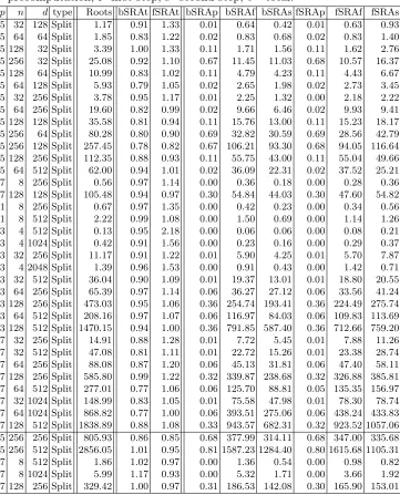
Table 2: Timings for selected parameters. The average total time needed by the full basic and fast SRA is provided as a quotient with respect to the average time needed by Roots; the other timings are given in seconds. bSRA=Basic SRA, fSRA=Fast SRA, p=precomputation, f=first step, s=second step, t= total.
p n d type Roots bSRAt fSRAt bSRAp bSRAf bSRAs fSRAp fSRAf fSRAs
5 32 128 Split 1.17 0.91 1.33 0.01 0.64 0.42 0.01 0.63 0.93
5 64 64 Split 1.85 0.83 1.22 0.02 0.83 0.68 0.02 0.83 1.40
5 128 32 Split 3.39 1.00 1.33 0.11 1.71 1.56 0.11 1.62 2.76 5 256 32 Split 25.08 0.92 1.10 0.67 11.45 11.03 0.68 10.57 16.37 5 128 64 Split 10.99 0.83 1.02 0.11 4.79 4.23 0.11 4.43 6.67 5 64 128 Split 5.93 0.79 1.05 0.02 2.65 1.98 0.02 2.73 3.45 5 32 256 Split 3.78 0.95 1.17 0.01 2.25 1.32 0.00 2.18 2.22 5 64 256 Split 19.60 0.82 0.99 0.02 9.66 6.46 0.02 9.93 9.41 5 128 128 Split 35.58 0.81 0.94 0.11 15.76 13.00 0.11 15.23 18.17 5 256 64 Split 80.28 0.80 0.90 0.69 32.82 30.59 0.69 28.56 42.79 5 256 128 Split 257.45 0.78 0.82 0.67 106.21 93.30 0.68 94.05 116.64 5 128 256 Split 112.35 0.88 0.93 0.11 55.75 43.00 0.11 55.04 49.66 5 64 512 Split 62.00 0.94 1.01 0.02 36.09 22.31 0.02 37.52 25.21
7 8 256 Split 0.56 0.97 1.14 0.00 0.36 0.18 0.00 0.28 0.36
7 128 128 Split 105.48 0.94 0.97 0.30 54.84 44.03 0.30 47.60 54.82 11 8 256 Split 0.67 0.97 1.35 0.00 0.42 0.23 0.00 0.34 0.56 11 8 512 Split 2.22 0.99 1.08 0.00 1.50 0.69 0.00 1.14 1.26 13 4 512 Split 0.13 0.95 2.18 0.00 0.06 0.06 0.00 0.08 0.21 13 4 1024 Split 0.42 0.91 1.56 0.00 0.23 0.16 0.00 0.29 0.37 13 32 256 Split 11.17 0.91 1.22 0.01 5.90 4.25 0.01 5.70 7.87 13 4 2048 Split 1.39 0.96 1.53 0.00 0.91 0.43 0.00 1.42 0.71 13 32 512 Split 36.04 0.90 1.09 0.01 19.37 13.01 0.01 18.80 20.55 13 64 256 Split 65.39 0.97 1.14 0.06 36.27 27.12 0.06 33.56 41.24 13 128 256 Split 473.03 0.95 1.06 0.36 254.74 193.41 0.36 224.49 275.74 13 64 512 Split 208.16 0.97 1.07 0.06 116.97 84.03 0.06 109.83 113.69 13 128 512 Split 1470.15 0.94 1.00 0.36 791.85 587.40 0.36 712.66 759.20 17 32 256 Split 14.91 0.88 1.28 0.01 7.72 5.45 0.01 7.88 11.26 17 32 512 Split 47.08 0.81 1.11 0.01 22.72 15.26 0.01 23.38 28.74 17 64 256 Split 88.08 0.87 1.20 0.06 45.13 31.81 0.06 47.40 58.11 17 128 256 Split 585.80 0.99 1.22 0.32 339.87 238.68 0.32 326.88 385.81 17 64 512 Split 277.01 0.77 1.06 0.06 125.70 88.81 0.05 135.35 156.97 17 32 1024 Split 148.99 0.83 1.05 0.01 75.58 47.98 0.01 78.30 78.74 17 64 1024 Split 868.82 0.77 1.00 0.06 393.51 275.06 0.06 438.24 433.83 17 128 512 Split 1838.89 0.88 1.08 0.33 943.57 682.31 0.32 923.52 1057.06 5 256 256 Split 805.93 0.86 0.85 0.68 377.99 314.11 0.68 347.00 335.68 5 256 512 Split 2856.05 1.01 0.95 0.81 1587.23 1284.40 0.80 1615.68 1105.31
7 8 512 Split 1.86 1.02 0.97 0.00 1.36 0.54 0.00 0.98 0.82
open problem to propose an optimized implementation of SRA together with parameters of practical interest for which SRA would consistently perform better than previous algorithms. On the algorithmic side, we believe that efficiency improvements can be achieved in SRA through a careful choice of the basis used in Lemma 1.
Our algorithm is radically different from previous ones. While traditional root-finding algorithms have used various strategies to separate the root set, SRA first “merges” the roots together using successive resultants with the polynomials xj+1−
(xpj−ajxj), and it then progressively separates them using gcds and root-finding
algo-rithms on polynomials of small degrees only. It would be interesting to explore alterna-tive merging strategies, in other words to take successive resultants with polynomials
xj+1−L˜j(xj) where the functions ˜Lj would be other non injective functions. An
al-ternative multipoint evaluation method could then be used instead of the dedicated Frobenius approach of Section 4.1 to preserve the resultant computation complexity with fast arithmetic.1
To conclude this paper, we would like to mention a very interesting and important open problem. This problem is the extension of our work to solvemultivariate polyno-mials f(x1, . . . , xm) = 0 under linear constraints xi ∈ Vi, where Vi ⊂ Fpn are vector spaces of dimensionn0 ≈n/moverFp. This problem is of great interest in cryptography,
to the factorization problem in SL(2,F2n) and to various discrete logarithm problems in small characteristic [6,7,11]. Following the same reasoning as in Section 3.1, we can write a polynomial system
f(x1,1, . . . , xm,1) = 0
xpij−aijxij =xi,j+1 i= 1, . . . , m;j= 1, . . . , n0−1
xpi,n0 −ai,n0xi,n0 = 0 i= 1, . . . , m
(6)
which includes the linear constraints and has a “block diagonal” structure. This system can clearly be solved by construction of new polynomialsf(i1,...,im) where the variables are successively replaced with resultants as well. However, we have not been able to design an algorithm that does not increase the degree of the new polynomials, and we could therefore not provide any good complexity bound. Nevertheless, we believe that this approach is very promising. Besides proving Petit and Quisquater’s conjecture to some extent [11], it may also lead to huge practical improvements on the cryptanalysis of ECDLP in characteristic 2 if the time and memory required to solve a multivariate polynomial with linear constraints were significantly decreased.
Acknowledgements The author would like to thank Tim Hodges, Sylvie Baudine and the program committee of ANTS for carefully reviewing previous versions of this paper. Nicolas Veyrat and Jean-Jacques Quisquater are also thanked for discussions related to this work. Finally, Jens Groth and Alan Lauder are thanked for hosting the author while writing this paper, respectively at University College London and University of Oxford. The research leading to these results has received funding from the Fonds National de
1
Fig.
1:
log
2
of
computing
times
(in
seconds)
for
Magma
R
o
ots
function,
b
as
ic
SRA,
fast
S
RA
and
their
main
comp
onen
t
parts.
The
graphs
displa
y
the
curv
es
for
sev
eral
d
v
Fig.
2:
log
2
of
computing
times
(in
seconds)
for
Magma
R
o
ots
function,
b
as
ic
SRA,
fast
S
RA
and
their
main
comp
onen
t
parts.
The
graphs
displa
y
the
curv
es
for
sev
eral
n
v
References
1. E. Berlekamp. Factoring polynomials over large finite fields.Mathematics of computation, 111:713– 735, 1970.
2. E. R. Berlekamp. Algebraic coding theory. Aegean Park Press, Laguna Hills, CA, USA, 1984. 3. Elwyn R. Berlekamp, H. Rumsey, and G. Solomon. On the solution of algebraic equations over
finite fields. Information and Control, 10(6):553–564, June 1967.
4. David G. Cantor and Hans Zassenhaus. A new algorithm for factoring polynomials over finite fields.
Mathematics of Computation, 36 (154):587592, 1981.
5. Yuanmi Chen and Phong Q. Nguyen. Faster algorithms for approximate common divisors: Breaking fully-homomorphic-encryption challenges over the integers. In Pointcheval and Johansson [12], pages 502–519.
6. Jean-Charles Faug`ere, Ludovic Perret, Christophe Petit, and Gu´ena¨el Renault. New subexponential algorithms for factoring in SL(2,2n). Cryptology ePrint Archive, Report 2011/598, 2011. http: //eprint.iacr.org/.
7. Jean-Charles Faug`ere, Ludovic Perret, Christophe Petit, and Gu´ena¨el Renault. Improving the complexity of index calculus algorithms in elliptic curves over binary fields. In Pointcheval and Johansson [12], pages 27–44.
8. Erich Kaltofen and Victor Shoup. Subquadratic-time factoring of polynomials over finite fields.
Math. Comput., 67(223):1179–1197, 1998.
9. Kiran S. Kedlaya and Christopher Umans. Fast polynomial factorization and modular composition.
SIAM J. Comput., 40(6):1767–1802, 2011.
10. Alfred Menezes, Paul C. van Oorschot, and Scott A. Vanstone. Subgroup refinement algorithms for root finding in GF(q).SIAM J. Comput., 21(2):228–239, 1992.
11. Christophe Petit and Jean-Jacques Quisquater. On polynomial systems arising from a Weil descent. In Xiaoyun Wang and Kazue Sako, editors,Asiacrypt, volume 7658 ofLecture Notes in Computer Science, pages 451–466. Springer, 2012.
12. David Pointcheval and Thomas Johansson, editors.Advances in Cryptology EUROCRYPT 2012 -31st Annual International Conference on the Theory and Applications of Cryptographic Techniques, Cambridge, UK, April 15-19, 2012. Proceedings, volume 7237 ofLecture Notes in Computer Science. Springer, 2012.
13. Michael O. Rabin. Probabilistic algorithms in finite fields. SIAM J. Comput., 9(2):273–280, 1980. 14. A. A. Sch¨onhage. Schnelle Berechnung von Kettenbruchentwicklungen.Acta Inf., 1:139–144, 1971. 15. Arnold Sch¨onhage. Schnelle Multiplikation von Polynomen ¨uber K¨orpern der Charakteristik 2.
Acta Informatica, 7 (4):395–398, 1977.
16. K. Thull and C. Yap. A unified approach to HGCD algorithms for olynomials and integers. Manuscript. Available fromhttp://cs.nyu.edu/cs/faculty/yap/allpapers.html/, 1990. 17. Paul C. van Oorschot and Scott A. Vanstone. A geometric approach to root finding in GF(qm).
IEEE Transactions on Information Theory, 35(2):444–453, 1989.
18. Joachim von zur Gathen and J¨urgen Gerhard. Modern Computer Algebra (2. ed.). Cambridge University Press, 2003.
19. Joachim von zur Gathen and Daniel Panario. Factoring polynomials over finite fields: A survey. J. Symb. Comput., 31(1/2):3–17, 2001.
20. Joachim von zur Gathen and Victor Shoup. Computing frobenius maps and factoring polynomials.
Computational Complexity, 2:187–224, 1992.
21. C. Fieker A. Steel (eds.) W. Bosma, J. J. Cannon. Handbook of Magma functions, edition 2.20. http://http://magma.maths.usyd.edu.au/magma/, 2013.
22. Virginia Vassilevska Williams. Multiplying matrices faster than coppersmith-winograd. In Howard J. Karloff and Toniann Pitassi, editors,STOC, pages 887–898. ACM, 2012.
A Magma SRA code
// recover parameters Rpol:=Parent(pol); Fq<x>:=BaseRing(Rpol); p:=Characteristic(Fq); n:=Degree(Fq);
d:=Degree(pol);
// precomputing part //
---R:=PolynomialRing(Fq,n,"lex");
AssignNames(~R,["Y" cat IntegerToString(ind): ind in [1..n]]);
// arbitrary choice of basis
basis := [x^ind: ind in [0..n-1]];
// equations relating the Yi variables Lval:=basis[1]^(p-1);
squareEq:=[];
for ind in [1..n-1] do // compute next
squareEq:=squareEq cat [(R.ind)^p - Lval*R.ind - R.(ind+1)] ;
// compute Lval = value of last equation evaluated at Y1=basis[ind] Lval:=R.1-basis[ind+1];
for ind2 in [1..ind] do
Lval:=NormalForm(squareEq[ind2],[Lval]); end for;
Lval:=-MonomialCoefficient(Lval,1)
/MonomialCoefficient(Lval,R.(ind+1)); Lval:=Lval^(p-1);
end for;
// compute last
squareEq:=squareEq cat [(R.n)^p - Lval*R.n] ;
// part depending on pol //
---pol:=(hom<Parent(pol) -> R | R.1>)(pol); polEq:=[pol];
// get an equation in R.n for var in [1..n-1] do
polEq:=polEq cat [pol]; end for;
// compute gcd of pol with last squareEq pol:=GCD(pol,squareEq[n]);
solEq:=[fac[1]: fac in Factorization(pol) | Degree(fac[1]) eq 1] ;
// successively recover values of Y_n-1, Y_n-2, etc for indvar in [n-ind+1: ind in [2..n]] do
newSolEq:=[];
for sol in solEq do
pol:=GCD(polEq[indvar],NormalForm(squareEq[indvar],[sol])); if Degree(pol) eq 1 then
newSolEq:= newSolEq cat [pol]; end if;
if Degree(pol) gt 1 then
newSolEq:= newSolEq cat [fac[1]: fac in
Factorization(pol) | Degree(fac[1]) eq 1] ; end if;
end for;
solEq:=newSolEq; end for;