Block Ciphers – Focus On The Linear Layer
(feat.
PRIDE
)
?Full Version
Martin R. Albrecht1??, Benedikt Driessen2? ? ?, Elif Bilge Kavun3†, Gregor Leander3‡, Christof Paar3, Tolga Yal¸cın4? ? ? 1
Information Security Group, Royal Holloway, University of London, UK
2 Infineon AG, Neubiberg, Germany 3
Horst G¨ortz Institute for IT Security, Ruhr-Universit¨at Bochum, Germany
4 University of Information Science and Technology, Ohrid, Macedonia
Abstract. The linear layer is a core component in any substitution-permutation network block cipher. Its design significantly influences both the security and the efficiency of the resulting block cipher. Surprisingly, not many general constructions are known that allow to choose trade-offs between security and efficiency. Especially, when compared to Sboxes, it seems that the linear layer is crucially understudied. In this paper, we propose a general methodology to construct good, sometimes optimal, linear layers allowing for a large variety of trade-offs. We give several instances of our construction and on top underline its value by presenting a new block cipher.PRIDEis optimized for 8-bit micro-controllers and significantly outperforms all academic solutions both in terms of code size and cycle count.
Keywords:block cipher, linear layer, wide-trail, embedded processors.
1
Introduction
Block ciphers are one of the most prominently used cryptographic primitives and probably account for the largest portion of data encrypted today. This was facilitated by the introduction of Rijndael as the Advanced Encryption Standard (AES) [2], which was a major step forward in the field of block cipher design. Not only does AES offer strong security, but its structure also inspired many cipher designs ever since. One of the merits of AES (and its predecessor SQUARE [20]) was demonstrating that a well-chosen linear layer is not only crucial for the security (and efficiency) of a block cipher, but also allows to argue in a simple and thereby convincing way about its security.
?
Corresponding author, [email protected]
??
Most of this work was done while the author was at the Technical University of Denmark
? ? ?
Most of this work was done while the authors were at Ruhr-Universit¨at Bochum.
†
The research was supported in part by the DFG Research Training Group GRK 1817/1.
‡
There are two main design strategies that can be identified for block ciphers: Sbox-based constructions and constructions without Sboxes, most prominently those using addition, rotation, and XORs (ARX designs). Furthermore, Sbox-based designs can be split intoFeistel-ciphers and substitution-permutation net-works (SPN). Both concepts have been successfully used in practice, the most prominent example of an SPN cipher being AES and the most prominent Feistel-cipher being the former Data Encryption Standard (DES) [22].
It is also worth mentioning that the concept of SPN has not only been used in the design of block ciphers but also for designing cryptographic permutations, most prominently for the design of several sponge-based hash functions including SHA-3 [11]. In SP networks, the round function consists of a non-linear layer composed of small Sboxes working in parallel on small chunks of the state and a linear layer that mixes those chunks. Thus, designing an SPN block cipher essentially reduces to choosing one (or several) Sboxes and a linear layer.
A lot of research has been devoted to the study of Sboxes. All Sboxes of size up to 4 bits have been classified (indeed, more than once – cf. [14,38,48]). Moreover, Sboxes with optimal resistance against differential and linear attacks have been classified up to dimension 5 [17]. In general, several constructions are known for good and optimal Sboxes in arbitrary dimensions. Starting with the work of Nyberg [45], this has evolved into its own field of research in which those functions are studied in great detail. A nice survey of the main results of this line of study is provided by Carlet [18].
The situation for the other main design part, the linear layer, is less clear.
1.1 The Linear Layer
For the design of the linear layer, two general approaches can be identified. One still widely-used method is to design the linear layer in a rather ad-hoc fashion, without following general design guidelines. While this might lead to very secure and efficient algorithms (cf. Serpent [3] and SHA-3 as prominent examples), it is not very satisfactory from a scientific point-of-view. The second general design strategy is the wide-trail strategy introduced by Daemen in [19] (see also [21]). Especially for the security against linear [43] and differential [12] attacks, the wide-trail strategy usually results in simple and strong security arguments. It is therefore not surprising that this concept has found its way in many recent designs (e.g. Khazad [9], Anubis [8], Grøstl [27], PHOTON [31], LED [32], PRINCE [16], mCrypton [41] to name but a few). In a nutshell, the main idea of the wide-trail strategy is to link the number of active Sboxes for linear and differential cryptanalysis to the minimal distance of a certain linear code associated with the linear layer of the cipher. In turn, choosing a good code (with some additional constraints) results in a large number of active Sboxes.
as the core component. This might guarantee an (partially) optimal number of active Sboxes, but usually comes at the price of a less efficient implementation. The only exception here is that, in the case of MDS matrices, the authors of PHOTON and LED made the observation that implementing such matrices in a serialized fashion improves hardware-efficiency. This idea was further generalized in [49,56], and more recently in [5].
It is our belief that, in many cases, it is advantageous to use a near-MDS matrix (or in general a matrix with a sub-optimal branch number) for the over-all design. Furthermore, it is, in our opinion, utmost surprising that there are virtually no general constructions or guidelines that would allow an SPN design to benefit from security vs. efficiency trade-offs. This is in particular important when it comes to ciphers where specific performance characteristics are crucial, e.g. in lightweight cryptography.
1.2 The Current State of Lightweight Cryptography
In recent years, the field of lightweight cryptography has attracted a lot of at-tention from the cryptographic community. In particular, designing lightweight block ciphers has been a very active field for several years now. The dominant metric according to which the vast majority of lightweight ciphers have been op-timized was and still is the chip area. While this is certainly a valid optimization objective, its relevance to real-world applications is limited. Nowadays, there are several interesting and strong proposals available that feature a very small area but simultaneously neglect other, important real-world constraints. Moreover, recent proposals achieve the goal of a small chip area by sacrificing execution speed to such an extent that even in applications where speed is supposedly uncritical, the ciphers are getting too slow1.
Note that software solutions, i.e. low-end embedded processors, actually dom-inate the world of embedded systems and dedicated hardware is a comparably small fraction. Considering this fact, it is quite puzzling that efficiency on low-cost processors was disregarded for so long. Certainly, there were a few ex-ceptions: Several theoretical and practical studies have already been done in this field. Practical examples include several proposals for instruction set ex-tensions [40,44,50,39]. Among these, the Intel AES instruction set [33] is the most well-known and practically relevant one. There have also been attempts to come up with ciphers that are (partially) tailored for low-cost processors [54,53,57,28,10,34]. Of these, execution times of both SEA and ITUbee are rather high, mostly due to the high number of rounds. Furthermore, ITUbee uses 8-bit Sboxes, which occupy a vast amount of program memory storage. SPECK, on the other hand, seems to be an excellentlightweight software cipher in terms of both speed and program memory.
It is obvious that there are quite some challenges to be overcome in this relatively untouched area of lightweight software cryptography. The software cipher for embedded devices of the future should not only be compact in terms
1
of program memory, but also be relatively fast in execution time. It should clearly be secure and, preferably, its security should be easily analysed and verified. The latter can possibly be achieved by building on conservative structures, which are conventionally costly in software implementation, thereby posing even harder challenges.
One major component influencing all or at least most of those criteria out-lined above is the linear layer. Thus, it is important to have general constructions for linear layers that allow to explore and make optimal use of the possible trade-offs.
1.3 Our Contribution
In this paper, we take steps towards a better understanding of possible trade-offs for linear layers. After introducing necessary concepts and notation in Section 2, we give a general construction that allows to combine several strong linear map-pings on a few number of bits into a strong linear layer for a larger number of bits (cf. Section 3). From a coding theory perspective, this construction corre-sponds to a construction known as block-interleaving (see [42], pages 131-132). While this idea is rather simple, its applicability is powerful. Implicitly, a spe-cific instance of our construction is already implemented in AES. Furthermore, special instances of this construction are recently used in [7] and [30].
We illustrate our approach by providing several linear layers with an optimal or almost optimal trade-off between hardware-efficiency and number of active Sboxes in Section 4. Along similar lines, we present a classification of all linear layers fulfilling the criteria of the block cipher PRINCE in Appendix C. Those examples show in particular that the construction given in Section 3 allows the construction of non-equivalent codes even when starting from equivalent ones. Secondly, we show that our construction also leads to very strong linear layers with respect to efficiency on embedded 8-bit micro-controllers. For this, we adopt a search strategy from [55] to find the most efficient linear layer possible within our constraints. We implemented this search on an FPGA platform to overcome the big computational effort involved and to have the advantage of reconfigurability. Details are described in Section 5.1.
2
Notation and Preliminaries
In this section, we fix the basic notation and furthermore recall the ideas of the wide-trail strategy.
We deal with SPN block ciphers where the Sbox layer consist ofnSboxes of size b each. Thus the block size of the cipher is n×b. The linear layer will be implemented by applyingk binary matrices in parallel.
We denote by F2 the field with two elements and by Fn2 the n-dimensional
vector space over F2. Note that any finite extension field F2b over F2 can be
viewed as the vector spaceFb
2of dimensionb. Along these lines, the vector space
(F2b)n can be viewed as the (nested) vector space Fb2 n
. Given a vectorx = (x1, . . . , xn) ∈ Fb2
n
where each xi ∈ Fb2 we define its
weight2 as
wtb(x) =|{1≤i≤n|xi6= 0}|.
Following [21], given a linear mapping L : (Fb2)n → (Fb2)n its differential
branch number is defined as
Bd(L) := min{wtb(x) + wtb(L(x))|x∈ Fb2 n
, x6= 0}.
The cryptographic significance of the branch number is that the branch number corresponds to the minimal number of active Sboxes in any two consecutive rounds. Here an Sbox is called active if it gets a non-zero input difference in its input.
Given an upper bound p on the differential probability for a single Sbox along with a lower bound of active Sboxes immediately allows to deduce an upper bound for any differential characteristic3using
average probability for any non-trivial characteristic ≤p#active Sboxes.
For linear cryptanalysis, the linear branch number is defined as Bl(L) := min{wtb(x) + wtb(L∗(x))| x∈ Fb2
n
, x6= 0}
where L∗ is the adjoint linear mapping. That is, with respect to the standard inner product, L∗ corresponds to the transposed matrix ofL.
In terms of correlation (cf., for example, [19]), an upper bound c on the absolute value of the correlation for a single Sbox results in a bound for any linear trail (or linear characteristic, linear path) via
absolute correlation for a trail ≤c#active Sboxes.
The differential branch number corresponds to the minimal distance of the
F2-linear codeC overFb2 with generator matrix
G= [I|LT]
2
Of course Fb2 n
is isomorphic toFnb2 , but the weight is defined differently on each. 3
where I is the n×n identity matrix. The length of the code is 2n and its dimension isn(here dimension corresponds to log2b(|C|) as it is not necessarily a linear code). Thus,Cis a (2n,2n) additive code over
Fb2with minimal distance
d=Bd(L).
The linear branch number corresponds in the same way to the minimal dis-tance of theF2-linear codeC⊥ with generator matrix
G∗= [L|I].
Note thatC⊥ is the dual code ofC and in general the minimal distances ofC⊥
andC do not need to be identical.
Finally, given linear mapsL1 andL2, we denote byL1×L2 the direct sum
of the mappings, i.e.
(L1×L2)(x, y) := (L1(x), L2(y)).
3
The Interleaving Construction
Following the wide-trail strategy, we construct linear layers by constructing a (2n,2n) additive codes with minimal distancedover
Fb2. The code needs to have
a generator matrixGin standard form, i.e.
G= [I|LT]
where the submatrixLis invertible, and corresponds to the linear layer we are using.
Hence, the main question is how to construct “efficient” matricesL with a given branch number. Our construction allows to combine small matrices into bigger ones. We hereby drastically reduce the search-space of possible linear layers. This in turn makes it possible to construct efficient linear layers for various trade-offs, as demonstrated in the following sections.
As mentioned above, the construction described in [21] can be seen as a special case of our construction. The main difference (except the generalization) is that we shift the focus of the construction in [21] from the 4 round super-box view to a 2 round-view. While Daemen and Rijmen focused on the bounds for 4 rounds, we make use of their ideas to actually construct linear layers. Moreover, a particular instance of the general construction we elaborate on here, was already used in the linear layer of the hash function Whirlwind [7]. There, several small MDS matrices are used to construct a larger one.
We give a simple illustrative example of our approach in Appendix A.
3.1 The General Construction
We are now ready to give a formal description of our approach. First define the following isomorphism
Pbn1,...bk:Fb21×F
b2
2 × · · · ×F
bk
2 n
→Fb21 n
×Fb22 n
× · · · ×Fb2k n
(x1, . . . , xn)7→
where xi=
x(1)i , . . . , x(ik) withx(ij)∈Fb2j.
This isomorphism performs the transformation of mapping Sbox outputs to our small linear layers Li. For example, in Appendix A, we considered individual bits (i.e.b1, . . . , bk= 1) from 4 (i.e.,k= 4) 4-bit Sboxes (i.en= 4).
Note that, for our purpose, there are in fact many possible choices forP. In particular, we may permute the entries within (Fb2i)
n. Given this isomorphism we can now state our main theorem. The construction ofP follows the idea of a diffusion-optimal mapping as defined in [21, Definition 5].
Theorem 1. LetGi= [I|LTi]be the generator matrix for anF2-linear(2n,2n)
code with minimal distance di over Fb2i for 0 ≤ i < k. Then the matrix G =
[I | LT] with
L= Pbn1,...bk−1
◦(L0×L1× · · · ×Lk−1)◦Pbn1,...bk
is the generator matrix of an F2-linear (2n,2n) code with minimal distance d
overFb
2 where
d= min
i di and b=
X
i
bi.
Proof. SincePbn1,...b
kand
Pbn1,...b
k
−1
are permutation matrices, by construction
Lhas full rank. To see that wtb(w) + wtb(v)≥minidi for anyv∈Fb2\ {0} and
w=L·v, observe that wtb(w) + wtb(v) is minimal when all entries inv are zero except those mapped to the positions acted on by Lj where Lj is the matrix
with the minimal branch number. ut
Remark 1. The interleaving construction allows to construct non-equivalent codes even when starting with equivalentLi’s. This is shown in a particular case in Ap-pendix C, where different choices of (equivalent)Li’s lead to different numbers of minimum-weight codewords.
A special case of the construction above is implicitly already used in AES. In the case of AES, it is used to construct a [8,4,5] code overF32
2 from 4 copies
of the [8,4,5] code overF8
2given by theMixColumnoperation. In the Superbox
view on AES, theShiftRows operation plays the role of the mappingP (and its inverse) and MixColumns corresponds to the mappingsLi.4
In the following, we use this construction to design efficient linear layers. Besides the differential and linear branch number, we hereby focus mainly on three criteria:
– Maximize the diffusion (cf. Section 3.3)
– Minimize the density of the matrix (cf. Section 4)
4 Note that the cipher PRINCE implicitly uses the construction twice. Once for
– Software-efficiency (cf. Section 5)
The strategy we employ is as follows. We first find candidates forL0, i.e.,
(2n,2n) additive codes with minimal distance d
0 over F2b0. In this stage, we
ensure that the branch number isd0 and our efficiency constraints are satisfied.
We then apply permutations toL0to produceLifori >0. This stage maximizes diffusion.
3.2 Searching for L0
The following lemma (which is a rather straightforward generalization of Theo-rem 4 in [56]) gives a necessary and sufficient condition that a given matrix L
has branch numberdoverFb2.
Lemma 1. LetLbe abn×bnbinary matrix, decomposed intob×bsubmatrices
Li,j.
L=
L0,0 L0,1 . . . L0,n−1
L1,0 L1,1 . . . L1,n−1
..
. ... . .. ...
Ln−1,0Ln−1,1. . . Ln−1,n−1
(1)
Then,Lhas differential branch numberdoverFb2if and only if alli×(n−d+i+1)
block submatrices of L have full rank for1≤i < d−1. Moreover,L has linear branch numberdif and only if all(n−d+i+ 1)×i block submatrices ofLhave full rank for1≤i < d−1.
Based on Lemma 1 we may instantiate various search algorithms which we will describe in Section 4 and Section 5. In our search we focus on cyclic ma-trices, i.e. matrices where row i > 0 is constructed by cyclic shifting row 0 by
iindices. These matrices have the advantage of being efficient both in software and hardware. Furthermore, since these matrices are symmetric, considering the dual codeC⊥ toC= [I| LT] is straightforward.
3.3 Ensuring High Dependency
In this section, we assume we are given a matrix L0 and wish to construct
L1, . . . , Lk−1 that maximize the diffusion of the mapL=
Pn
b1,...bk
−1
◦(L0×
L1× · · · ×Lk−1)◦Pbn1,...bk.
Given anbn×bn binary matrix L decomposed as in Eq. (1), we define its support as the n×nbinary matrix Supp(L) where
Supp(L)i,j =
1 ifLi,j6= 0 0 else
Now assume that Supp(L0) has a zero entry at indexi0, j0. If we apply the same
impact on the inputs of the j0th Sbox after the linear layer. In other words, a linear-layer following the construction of Theorem 1 ensure full dependency if and only if
_
0≤i<k
Supp(Li)
i0,j0
= 1 ∀ 0≤i0, j0< n.
Hence, we want to apply different matrices Li in each of the k positions, such that in at least one Supp(Li) has a non-zero entry at indexi0, j0 for all 0≤
i0, j0 < n. In order to construct matricesLi fori >0 from a matrixL0 we may
apply block-permutation matrices from the left and right toL0as these clearly
neither impact the density nor the branch number. Hence, we focus on finding permutation matrices Pi, Qi such that the density of W0≤i<bSupp(Pi·L0·Qi)
is maximized. In Appendix F, we give two strategies for finding such Pi,Qi, one is heuristic but computationally cheap, the other is guaranteed to return an optimal solution – based on Constraint Integer Programming – but can be computationally intensive.
We note that the difficulty of the problem depends on the size of the Sbox and the density of Li. As MDS matrices always have density 1, the problem of full dependency does not occur when combining such matrices. Finally, if the construction ensures full dependency for a given k, it is always possible to achieve full dependency for anyk0≥k.
In contrast with the branch number, if a linear layer ensures high dependency, its inverse does not necessarily achieve the same dependency. Thus, it is in general necessary to check the dependency of the inverse separately.
4
Optimizing for Hardware
In this section, we give examples of [2n, n, d] codes overFb2 and give algorithms
for finding such instances. First, the following lemma gives a lower bound on the density of a matrix with branch number d. Our aim here is to find linear layers that are efficiently implementable in hardware. More precisely, we aim for an implementation in one cycle. PHOTON and LED demonstrated that there is a trade-off between clock cycles and number of gate equivalence for the linear layer. The trade-off we consider here is, complementary to PHOTON and LED, between efficient implementation in one clock cycle and the (linear and differential) branch number. Note that in our setting, the cost of implementation is directly connected to the number of ones in the matrix representation of the linear layer.
Lemma 2. Let matrix G= [I | LT] be the generator matrix for an
F2-linear
of [I |LT] isd. Hence, there must be at leastd−1 ones per row. Applying the same argument tow=LT·v=v·Lshows that at leastd−1 entries per column
must be non-zero. ut
The main merit of the above lemma is that it allows to determine the opti-mal solutions in terms of efficiency. This is in contrast to the case for software implementation, where the optimal solution is unknown.
Lemmas 1 and 2 give rise to various search strategies for finding (2n,2n) additive codes with minimal distance dover Fb2. We discuss those strategies in
Appendix B and present results of those strategies next.
4.1 Hardware-Optimal Examples
Below we give some examples for our construction. We hereby focus on [2n, n, d] codes overF2, i.e. we usebi = 1.5 Note that this naturally limits the achievable branch number. For binary linear codes the optimal minimal distance is known for small length (cf. [29] for more information). We give a small abridgement of the known bounds on the minimal distance for linear [2n, n] codes overF2,F4,
and F8 in Appendix E. As can be seen in this table, in order to achieve a high
branch number, it might be necessary to consider linear codes overF2m, or (more general) additive codes overFm
2 for some smallm >1.
The examples in Figure 1 are optimal in the sense that they achieve the best possible branch number (both linear and differential) for the given length (with the exception of n= 11,13, and 14) with the least possible number of ones in the matrix (cf. Lemma 2). The numberDcorresponds to the average number of ones per row/column andDinv to the average number of ones per row/column of the inverse matrix. The only candidate which does not satisfy D =d−1 is
n= 8. This candidate was found using the approach from Appendix B.3, which guarantees to return the optimal solution. Hence, we conclude that 418 is indeed the lowest density possible. That is, there is no 8×8 binary matrix with branch number 5 with only 32 ones, but the best we can do is 33 ones.
For each example we list the dimension (i.e the number of Sboxes), the achieved branch number and the minimalksuch that it is possible to achieve full dependency with two Sbox layers interleaved with one linear layer. These values were found using the CIP approach in Section 3.3. Note that in this case (i.e.
bi = 1) the value k actually corresponds to the minimal Sbox size that allows full dependency. Finally,kinvis the minimum Sbox size to achieve full diffusion for the inverse matrix. Note that for all these examples, the corresponding code is actually equivalent to its dual. In particular this implies that the linear and differential branch number are equal.
5 We refer to Appendix C for an exemplary comparison of the set of linear layers
nmax(d) d D Dinv k kinvTechniqueMatrix
2 2 2 1 1 2 2 App. B.1 cyclic shift (10) to the left. 3 2 2 1 1 3 3 App. B.1 cyclic shift (100) to the left. 4 4 4 3 3 2 2 App. B.1 cyclic shift (1110) to the left. 5 4 4 3 3 2 2 App. B.1 cyclic shift (11100) to the left. 6 4 4 3 3 2 2 App. B.1 cyclic shift (110100) to the left. 7 4 4 3 437 3 2 App. B.3 in Figure 2
8 5 5 418 478 3 2 App. B.3 in Appendix F.3
9 6 6 5 56
9 2 2 App. B.3 in Figure 2
10 6 6 5 5 2 2 App. B.1 cyclic shift (1111010000) to the left. 11 7 6 5 5 3 3 App. B.1 cyclic shift (11110100000) to the left. 12 8 8 7 7 2 2 App. B.1 cyclic shift (110111101000) to the left. 13 7 6 5 5 ≤4≤4 App. B.1 cyclic shift (1110110000000) to the left. 14 8 6 5 5 ≤4≤4 App. B.1 cyclic shift (11101010000000) to the left. 15 8 8 7 7 3 3 App. B.1 cyclic shift (101101110010000) to the left. 16 8 8 7 7 3 3 App. B.1 cyclic shift (1111011010000000) to the left.
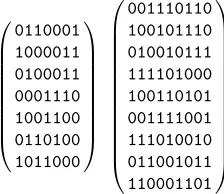
Fig. 1.Examples of hardware efficient linear layers overF2
0110001 1000011 0100011 0001110 1001100 0110100 1011000
001110110 100101110 010010111 111101000 100110101 001111001 111010010 011001011 110001101
Fig. 2.Examples of [14,7,4] and [18,9,6] codes overF2.
5
Software-Friendly Examples and the Cipher
PRIDE
In this section, we describe our new lightweight software-cipherPRIDE, a 64-bit block cipher that uses a 128-bit key. We refer to Appendix D for a sketch of the security analysis and to the full version for more details.
The target platform of PRIDE is Atmel’s AVR micro-controller [4], as it is dominating the market along with PIC [46] (see [47]). Furthermore, many implementations in literature are also implemented in AVR, we therefore opt for this platform to provide a better comparison to other ciphers (including SIMON and SPECK [10]). However, the reconfigurable nature of our search architecture (cf. Section 5.1) to find the basic layers of the cipher allows us to extend the search to various platforms in the future.
5.1 The Search for The Linear Layer
A natural choice in terms of Theorem 1 is to choosek= 4 and b1 =b2=b3=
b4= 1. Thus, the task reduces to find four 16×16 matrices forming one 64×64
matrix (to permute the whole state) of the following form:
L0 0 0 0
0 L1 0 0
0 0 L2 0
0 0 0 L3
Each of these four 16×16 matrices should provide branch number 4 and together achieve high dependency with the least possible number of instructions. Instead of searching for an efficient implementation for a given matrix, we decided to search for the most efficient solution fulfilling our criteria.
To find such matrices (Li) that could be implemented very efficiently given the AVR instruction set, we performed an extensive and hardware-aided tree search. Our search engine was optimized to look for AVR assembly code seg-ments utilizing a limited set of instructions that would result in linear behaviour at matrix level. These are namely CLC, EOR, MOV, MOVW, CLR, SWAP, ASR, ROR, ROL, LSR, and LSL instructions. As we are looking for 16×16 matrices, the state to be multiplied with eachLi is stored in two 8-bit registers, which we call X and Y. We also allowed utilization of four temporary regis-ters, namelyT0,T1,T2, andT3. We designed and optimized our search engine according to these registers. Our search engine checks the resulting matrix Li afterN instructions to see if it provides the desired characteristics. While trying to reach instruction N, we try all possible instruction-register combinations in each step. This of course comes with an impractical time complexity, especially when N is increased further. To deal with this time complexity, we came up with several optimizations. As a first step, we limited the utilization of certain instruction-register combinations. For example, we excluded CLC and CLR in-structions from the combinations for the first and last inin-structions. Also, EOR is not considered in the first instruction. Again, for the first and last instruc-tions, SWAP, ASR, ROR, ROL, LSR, and LSL instructions are only used with
X andY. Furthermore, we did not allow temporary registers as the destination while trying MOV and MOVW instructions in the last instruction andX −Y
However, such optimizations were not enough to reduce the time complexity. We therefore applied further optimizations, i.e., when the matrices of all registers do not give full rank, we stop the search as we know that we cannot find an invertible linear layer any more.
In the end, we found matrices that fulfil all of our criteria starting from 7 instructions.
We implemented our search architecture on a Xilinx ML605 (Virtex-6 FPGA) evaluation board. The reconfigurable nature of the FPGA allowed us to change easily between different parameters, i.e. the number of instructions. The details of this search engine can be found in [35].
5.2 An Extremely Efficient Linear Layer
As a result of the search explained in Section 5.1, we achieved an extremely effi-cient linear layer. The cheapest solution provided by our search needed 36 cycles for the complete linear layer, which is what we opted for. The optimal matrices forming the linear layer are given in the Appendix G. Of these four matrices,
L0 andL3are involutions with the cost of 7 instructions (in turn, clock cycles),
while L1 and L2 require 11 and 13 instructions for true and inverse matrices,
respectively. The assembly codes are given in Appendix H to show the claimed number of instructions.
Comparing to linear layers of other SPN-based ciphers clearly demonstrated the benefit of our approach. Note however, that these comparisons have to be taken with care as not all linear layers operate on the same state size and do not offer the same security level. The linear layer of the ISO-standard lightweight cipher PRESENT [15] costs 144 cycles (derived from the total cycle count given in [25]). MixColumns operation of NIST-standard AES6 costs 117 instructions
(but 149 cycles because of 3-cycle data load instruction utilizations, as Mix-Columns constants are implemented as look-up table – which means additional 256 bytes of memory, too) [6]. Note that ShiftRows operation was merged with the look-up table of Sbox in this implementation, so we take only MixColumns cost as the linear layer cost. The linear layer of another ISO-standard lightweight cipher CLEFIA [51] (again 128-bit cipher) costs 146 instructions and 668 cycles. Bit-sliced oriented design Serpent (AES finalist, 128-bit cipher) linear layer costs 155 instructions and 158 cycles. Other lightweight proposals, KLEIN [28] and mCrypton linear layers cost 104 instructions (100 cycles) and 116 instructions (342 cycles), respectively [24]. Finally, the linear layer cost of PRINCE is 357 in-structions and 524 cycles7, which is even worse than AES. One of the reasons for
this high cost is the non-cyclic 4×4 matrices forming the linear layer. The other reason is the ShiftRows operation applied on 4-bit state words, which makes coding much more complex than that of AES on an 8-bit micro-controller.
6 It is of course not fair to compare a 128-bit cipher with a 64-bit cipher. However, we
provide AES numbers as a reference due to the fact that it is a widely-used standard cipher and its cost is much better compared to many lightweight ciphers.
7
5.3 Sbox Selection
For our bit-sliced design, we decided to use a very simple (in terms of software-efficiency – the formulation is given in Appendix I) 10-instruction Sbox (which makes 10×2 = 20 clock cycles in total for the whole state). It is at the same time an involution Sbox, which prevents the encryption/decryption overhead. Besides being very efficient in terms of cycle count, this Sbox is also optimal with respect to linear and differential attacks. The maximal probability of a differential is 1/4 and the best correlation of any linear approximation is 1/2. ThePRIDESbox is given below.
x 0x0 0x1 0x2 0x3 0x4 0x5 0x6 0x7 0x8 0x9 0xa 0xb 0xc 0xd 0xe 0xf S(x) 0x0 0x4 0x8 0xf 0x1 0x5 0xe 0x9 0x2 0x7 0xa 0xc 0xb 0xd 0x6 0x3
The assembly codes are given in Appendix H to show the claimed number of instructions.
5.4 Description of PRIDE
Similar to PRINCE, the cipher makes use of the FX construction [36,13]. A pre-whitening keyk0 and post-whitening keyk2are derived from one half ofk,
while the second half serves as basisk1 for the round keys, i.e.,
k=k0||k1 with k2=k0.
Moreover, in order to allow an efficient bit-sliced implementation, the cipher starts and ends with a bit-permutation. This clearly does not influence the se-curity of PRIDEin any way. Note that in a bit-sliced implementation, none of the permutations P norP−1 used in PRIDE has to be actually implemented explicitly. The cipher has 20 rounds, of which the first 19 are identical. Subkeys are different for each round, i.e., the subkey for round i is given byfi(k1). We
define
fi(k1) =k10||g
(0)
i (k11)||k12||g
(1)
i (k13)||k14||g
(2)
i (k15)||k16||g
(3)
i (k17)
as the subkey derivation function with four byte-local modifiers of the key as
gi(0)(x) = (x+ 193i) mod 256, g(1)i (x) = (x+ 165i) mod 256, gi(2)(x) = (x+ 81i) mod 256, gi(3)(x) = (x+ 197i) mod 256,
which simply add one of four constants to every other byte of k1. The overall
The round functionRof the cipher shows a classical substitution-permutation network: The state is XORed with the round key, fed into 16 parallel 4-bit Sboxes and then permuted and processed by the linear layer.
The difference between Rand R0 is that in the latter no more diffusion is
necessary, therefore the last round ends after the substitution layer. With the software-friendly matrices we have found as described above, the linear layer is defined as follows (cf. Theorem 1 and Appendix G):
L:=P−1◦(L0×L1×L2×L3)◦P where P :=P116,1,1,1.
The test vectors for the cipher are provided in the Appendix J.
5.5 Performance Analysis
As depicted above, one round of our proposed cipherPRIDEconsists of a linear layer, a substitution layer, a key addition, and a round constant addition (key update). In a software implementation ofPRIDEon a micro-controller, we also perform branching in each round of the cipher in addition to the previously listed layers. Adding up all these costs gives us the total implementation cost for one round of the cipher. The total cost can roughly be calculated by multiplying the number of rounds with the cost of each round. Note that we should subtract the cost of one linear layer from the overall cost, asPRIDEhas no linear layer in the last round. The software implementation cost of the round function of
PRIDEon Atmel AVR ATmega8 8-bit micro-controller [4] is presented in the
following:
Key
up
date
Key
addition
Sb
o
x
La
y
er
Linear
La
y
er
T
otal
Time (cycles) 4 8 20 36 68
ComparingPRIDEto existing ciphers in literature, we can see that it out-performs many of them significantly both in terms of cycle count and code size. Note that we are not using any look-up tables in our implementation, in turn no RAMs8. The comparison with existing implementations is given below:
AES-128
[25]
SERPENT-128
[25]
PRESENT-128
[25]
CLEFIA-128
[25]
SEA-96
[53]
NOEKEON-128
[24]
PRINCE-128 ITUb
ee-80
[34]
SIMON-64/128
[10]
SPECK-64/96
[10]
SPECK-64/128
[10]
PRIDE
t(cyc) 3159 49314 10792 28648 17745 23517 3614 2607 2000 1152 1200 1514
bytes 1570 7220 660 3046 386 364 1108 716 282 182 186 266
eq.r. 5/10 1/32 4/31 1/18 8/92 1/16 5/12 12/20 33/44 34/26 34/27 In the table, the first row is the time (performance) in clock cycles, the second row is the code size in bytes, and the third row is the equivalent rounds. The third row expresses the number of rounds for the given ciphers that would result in a total running time similar toPRIDE.
Note that, as we did not come across to any reference implementations in the literature, we implemented PRINCE in AVR for comparison. We also do not list the RAM utilization for the ciphers under comparison in the table.
In the implementation ofPRIDE, our target was to be fast and at the same time compact. Note that we do not exclude data & key read and data write back as well as the whitening steps in our results (these are omitted in SIMON and SPECK numbers). Although the given numbers are just for encryption, decryption overhead is also acceptable: It costs 1570 clock cycles and 282 bytes. A cautionary note is indicated for the above comparison for several reasons. AES, SERPENT, CLEFIA, and NOEKOEN are working on 128-bit blocks; so, for a cycle per byte comparison, their cycle count has to be divided by a factor of two. Moreover, the ciphers differ in the claimed security level and key-size.
PRIDEdoes not claim any resistance against related-key attacks (and actually
can be distinguished trivially in this setting) and also generic time-memory trade-offs are possible againstPRIDEin contrast to most other ciphers. Besides those restrictions, the security margin inPRIDEin terms of the number of rounds is (in our belief) sufficient.
One can see that PRIDE is comparable to 64/96 and SPECK-64/128 (members of NSA’ssoftware-cipher family), which are based on a Feistel structure and use modular additions as the main source of non-linearity.
In addition to the above table, the recent work of Grosso et al. [30] presents LS-Designs. This is a family of block ciphers that can systematically take
ad-8
vantage of bit-slicing in a principled manner. In this paper, the authors make use of look-up tables. Therefore, a direct comparison withPRIDEis not fair as the use of look-up tables does not minimize the linear layer cost. However, to have an idea, we can try to estimate the cost of the 64-bit case of this family. They suggest two options: The first uses 4-bit Sbox with 16-bit Lbox, and the second uses 8-bit Sbox with 8-bit Lbox. The first option has 8 rounds, which results in 64 non-linear operations, 128 XORs, and 128 table look-ups in total. The second one has 6 rounds, which takes 72 non-linear operations, 144 XORs, and 48 table look-ups. For linear layer cost, we consider the XOR cost together with table look-ups. Unfortunately, it is not easy to estimate the overall cost of the given two options on AVR platform as the table look-ups take more than one cycle compared to the non-linear and linear operations. Another important point here to mention is that the use of look-up tables result in a huge memory utilization.
Finally, we note that, despite its target being software implementations,
PRIDE is also efficient in hardware. It can be considered a hardware-friendly
design, due to its cheap linear and Sbox layers.
6
Conclusion
In this work, we have presented a framework for constructing linear layers for block ciphers which allows to trade security against efficiency. For a given se-curity level, in our case we focused on the branch number, we demonstrated techniques to find very efficient linear layers satisfying this security level. Us-ing this framework, we presented a family of linear layers that are efficient in hardware. Furthermore, we presented a new cipher PRIDEdedicated for 8-bit micro-controllers that offers competitive performance due to our new techniques for finding linear layers.
One important question is on the optimality of a given construction for a linear layer. In particular, in the case of our construction, the natural ques-tion is if the reducques-tion of the search space excludes optimal soluques-tions and only sub-optimal solutions remain. For the hardware-friendly examples presented in Section 4 and Appendix C, it is easy to argue that those constructions are opti-mal. Thus, in this case the reduction of the search space clearly did not have a negative influence on the results. In general, and for the linear layer constructed in Section 5 in particular, the situation is less clear. The main reason is that, again, the construction of linear layers is understudied and hence we do not have enough prior work to answer this question satisfactorily at the moment. Instead we view the PRIDE linear layer as a strong benchmark for efficient linear layers with the given parameters and encourage researchers to try to beat its performance.
has the potential to significantly increase the number of active Sboxes when combined with a linear layer based on Theorem 1. Finding ways to easily prove such a result is worth investigating.
Finally, regardingPRIDE, we obviously encourage further cryptanalysis.
References
1. Tobias Achterberg.Constraint Integer Programming. PhD thesis, TU Berlin, 2007. 2. AES. Advanced Encryption Standard. FIPS PUB 197, Federal Information
Pro-cessing Standards Publication, 2001.
3. Ross Anderson, Eli Biham, and Lars Knudsen. Serpent: A Proposal for the Ad-vanced Encryption Standard, 1998.
4. Atmel AVR. ATmega8 Datasheet. http://www.atmel.com/images/doc8159.pdf. 5. Daniel Augot and Matthieu Finiasz. Direct Construction of Recursive MDS
Dif-fusion Layers using Shortened BCH Codes. In Fast Software Encryption (FSE), LNCS. Springer, 2014, to appear.
6. AVRAES: The AES block cipher on AVR controllers. http://point-at-infinity.org/avraes/.
7. Paulo S. L. M. Barreto, Ventzislav Nikov, Svetla Nikova, Vincent Rijmen, and Elmar Tischhauser. Whirlwind: A New Cryptographic Hash Function. Des. Codes Cryptography, 56(2-3):141–162, 2010.
8. Paulo S.L.M. Barreto and Vincent Rijmen. The Anubis Block Cipher. Submission to the NESSIE project, 2001.
9. Paulo S.L.M. Barreto and Vincent Rijmen. The Khazad Legacy-level Block Cipher. Submission to the NESSIE project, 2001.
10. Ray Beaulieu, Douglas Shors, Jason Smith, Stefan Treatman-Clark, Bryan Weeks, and Louis Wingers. The SIMON and SPECK Families of Lightweight Block Ci-phers. IACR Cryptology ePrint Archive, 2013:414, 2013.
11. Guido Bertoni, Joan Daemen, Micha¨el Peeters, and Gilles Van Assche. Keccak Specifications, 2009.
12. Eli Biham and Adi Shamir. Differential Cryptanalysis of DES-like Cryptosystems. InCRYPTO, volume 537 ofLNCS, pages 2–21. Springer, 1990.
13. Alex Biryukov. DES-X (or DESX). InEncyclopedia of Cryptography and Security (2nd Ed.), page 331. Springer, 2011.
14. Alex Biryukov, Christophe De Canni`ere, An Braeken, and Bart Preneel. A Toolbox for Cryptanalysis: Linear and Affine Equivalence Algorithms. In EUROCRYPT, volume 2656 ofLNCS, pages 33–50. Springer, 2003.
15. Andrey Bogdanov, Lars R. Knudsen, Gregor Leander, Christof Paar, Axel Poschmann, Matthew J. B. Robshaw, Yannick Seurin, and Charlotte Vikkelsø. PRESENT: An Ultra-Lightweight Block Cipher. InCryptographic Hardware and Embedded Systems - CHES 2007, volume 4727 ofLNCS, pages 450–466. Springer, 2007.
17. Marcus Brinkmann and Gregor Leander. On the Classification of APN Functions Up to Dimension Five. Des. Codes Cryptography, 49(1–3):273–288, 2008.
18. Claude Carlet. Boolean Methods and Models, chapter Vectorial Boolean Functions for Cryptography. Cambridge University Press, 2010.
19. Joan Daemen.Cipher and Hash Function Design, Strategies Based On Linear and Differential Cryptanalysis. PhD thesis, Katholieke Universiteit Leuven, 1995. 20. Joan Daemen, Lars Knudsen, and Vincent Rijmen. The Block Cipher SQUARE.
InFast Software Encryption (FSE), LNCS. Springer, 1997.
21. Joan Daemen and Vincent Rijmen. The Wide Trail Design Strategy. InIMA Int. Conf., volume 2260 of LNCS, pages 222–238. Springer, 2001.
22. DES. Data Encryption Standard. FIPS PUB 46, Federal Information Processing Standards Publication, 1977.
23. Stefan Dodunekov and Ivan Landgev. On near-MDS codes. Journal of Geometry, 54(1):30–43, 1995.
24. Thomas Eisenbarth, Zheng Gong, Tim G¨uneysu, Stefan Heyse, Sebastiaan In-desteege, St´ephanie Kerckhof, Fran¸cois Koeune, Tomislav Nad, Thomas Plos, Francesco Regazzoni, Fran¸cois-Xavier Standaert, and Loic van Oldeneel tot Olden-zeel. Compact Implementation and Performance Evaluation of Block Ciphers in ATtiny Devices. In AFRICACRYPT, volume 7374 of LNCS, pages 172–187. Springer, 2012.
25. Susanne Engels, Elif Bilge Kavun, Hristina Mihajloska, Christof Paar, and Tolga Yal¸cın. A Non-Linear/Linear Instruction Set Extension for Lightweight Block Ciphers. In ARITH’21: 21st IEEE Symposium on Computer Arithmetics. IEEE Computer Society, 2013.
26. Jean-Charles Faug`ere. A New Efficient Algorithm for Computing Gr¨obner Basis (F4). Journal of Pure and Applied Algebra, 139(1-3):61–88, 1999.
27. P. Gauravaram, L. Knudsen, K. Matusiewicz, F. Mendel, C. Rechberger, M. Schl¨aer, and S. Thomsen. Grøstl. SHA-3 Final-round Candidate, 2009. 28. Zheng Gong, Svetla Nikova, and Yee Wei Law. KLEIN: A New Family of
Lightweight Block Ciphers. In RFID Security and Privacy (RFIDSec), volume 7055 ofLNCS, pages 1–18. Springer, 2011.
29. Markus Grassl. Bounds On the Minimum Distance of Linear Codes and Quantum Codes. Online available athttp://www.codetables.de, 2007.
30. Vincent Grosso, Ga¨etan Leurent, Fran¸cois-Xavier Standaert, and Kerem Varıcı. LS-Designs: Bitslice Encryption for Efficient Masked Software Implementations. InFast Software Encryption (FSE), LNCS. Springer, 2014, to appear.
31. Jian Guo, Thomas Peyrin, and Axel Poschmann. The PHOTON Family of Lightweight Hash Functions. In Advances in Cryptology - CRYPTO 2011, vol-ume 6841 ofLNCS, pages 222–239. Springer, 2011.
32. Jian Guo, Thomas Peyrin, Axel Poschmann, and Matthew J. B. Robshaw. The LED Block Cipher. InCryptographic Hardware and Embedded Systems (CHES), pages 326–341, 2011.
33. Intel. Advanced Encryption Standard Instructions. (Intel AES-NI), 2008.
34. Ferhat Karako¸c, H¨useyin Demirci, and Emre Harmancı. ITUbee: A Software Ori-ented Lightweight Block Cipher. InSecond International Workshop on Lightweight Cryptography for Security and Privacy (LightSec), 2013.
36. Joe Kilian and Phillip Rogaway. How to Protect DES Against Exhaustive Key Search (An Analysis of DESX). J. Cryptology, 14(1):17–35, 2001.
37. Miroslav Kneˇzevi´c, Ventzislav Nikov, and Peter Rombouts. Low-Latency Encryp-tion - Is ”Lightweight = Light + Wait”? In CHES, volume 7428 ofLNCS, pages 426–446. Springer, 2012.
38. Gregor Leander and Axel Poschmann. On the Classification of 4 Bit S-Boxes. In WAIFI, volume 4547 ofLNCS, pages 159–176. Springer, 2007.
39. Ruby B. Lee, Murat Fı¸skıran, Michael Wang, Yedidya Hilewitz, and Yu-Yuan Chen. PAX: A Cryptographic Processor with Parallel Table Lookup and Wordsize Scalability. Princeton University Department of Electrical Engineering Technical Report CE-L2007-010, 2007.
40. Ruby B. Lee, Zhijie Shi, and Xiao Yang. Efficient Permutation Instructions for Fast Software Cryptography. IEEE Micro, 21(6):56–69, 2001.
41. Chae Lim and Tymur Korkishko. mCrypton – A Lightweight Block Cipher for Se-curity of Low-Cost RFID Tags and Sensors. InInformation Security Applications, volume 3786 ofLNCS, pages 243–258. Springer, 2006.
42. Shu Lin and Daniel J. Costello, editors. Error Control Coding (2nd Edition). Prentice Hall, 2004.
43. Mitsuru Matsui. Linear Cryptoanalysis Method for DES Cipher. InEUROCRYPT, volume 765 ofLNCS, pages 386–397. Springer, 1993.
44. John Patrick McGregor and Ruby B. Lee. Architectural Enhancements for Fast Subword Permutations with Repetitions in Cryptographic Applications. In 19th International Conference on Computer Design (ICCD 2001), pages 453–461, 2001. 45. Kaisa Nyberg. Differentially Uniform Mappings for Cryptography. In
EURO-CRYPT, volume 765 ofLNCS, pages 55–64. Springer, 1993. 46. PIC. 12-Bit Core Instruction Set.
47. PIC vs. AVR. http://www.ladyada.net/library/picvsavr.html.
48. Markku-Juhani O. Saarinen. Cryptographic Analysis of All 4×4-Bit S-Boxes. InSelected Areas in Cryptography (SAC), volume 7118 of LNCS, pages 118–133. Springer, 2011.
49. Mahdi Sajadieh, Mohammad Dakhilalian, Hamid Mala, and Pouyan Sepehrdad. Recursive Diffusion Layers for Block Ciphers and Hash Functions. InFast Software Encryption (FSE), volume 7549 ofLNCS, pages 385–401. Springer, 2012. 50. Zhijie Jerry Shi, Xiao Yang, and Ruby B. Lee. Alternative Application-Specific
Processor Architectures for Fast Arbitrary Bit Permutations. IJES, 3(4):219–228, 2008.
51. Taizo Shirai, Kyoji Shibutani, Toru Akishita, Shiho Moriai, and Tetsu Iwata. The 128-bit Block Cipher CLEFIA (Extended Abstract). InFast Software Encryption (FSE), volume 4593 ofLNCS, pages 181–195. Springer, 2007.
52. Mate Soos. CryptoMiniSat 2.9.6. https://github.com/msoos/cryptominisat, 2013. 53. Fran¸cois-Xavier Standaert, Gilles Piret, Neil Gershenfeld, and Jean-Jacques Quisquater. SEA: a Scalable Encryption Algorithm for Small Embedded Applica-tions. InWorkshop on Lightweight Crypto, 2005.
54. Tomoyasu Suzaki, Kazuhiko Minematsu, Sumio Morioka, and Eita Kobayashi. TWINE: A Lightweight Block Cipher for Multiple Platforms. InSelected Areas in Cryptography (SAC), volume 7707 ofLNCS, pages 339–354. Springer, 2012. 55. Markus Ullrich, Christophe De Canni`ere, Sebastiaan Indesteege, ¨Ozg¨ul K¨u¸c¨uk,
56. Shengbao Wu, Mingsheng Wang, and Wenling Wu. Recursive Diffusion Layers for (Lightweight) Block Ciphers and Hash Functions. InSelected Areas in Cryptogra-phy (SAC), volume 7707 ofLNCS, pages 355–371. Springer, 2012.
Appendices
A
An Example for the Interleaving Construction
Our example takes its cue from the cipher PRINCE. Assume we want to con-struct a linear layerLworking on 4 chunks of 4 bits with linear- and differential branch number 4. That is, we want to construct an (8,24) additive code with
minimal distance 4 overF42 such that the dual code has minimum distance 4 as
well. As a further requirement in this example, we want to focus on the hardware-efficiency, i.e. we would like to reduce the number of ones in the corresponding matrix to a minimum. Lastly, we also would like to ensure good diffusion. More precisely, after two Sbox layers interleaved with one linear layer we require that each bit of the output depends on each bit of the input.
It is not hard to see that (as a matrix) L needs to have at least 3 ones in each row and column (cf. Lemma 2 in Section 4). We thus face the problem of finding an invertible 16×16 binary matrix with branch number 4 and exactly 3 ones in each row and column9. As there are 2256 16×16 matrices, the search
space is a priori huge.
The basic idea of our construction (depicted below) is simply to first re-group the output bits of the Sbox layer.
We collect all first output bits of each Sbox, all second bits, all third bits, and all fourth bits. Next, we apply independently 4 linear mappings on 4 bits, i.e. we multiply each 4-bit chunk with a 4×4 binary matrix. Afterwards the bits are again re-grouped, and the process is repeated.
The key point (cf. Theorem 1 for the general statement) is that the linear (resp. differential) branch number of the entire linear layer (using wt4) equals the
minimal linear (resp. differential) branch number of the 4 small binary matrices (using wt1). Moreover, the number of ones in each row and column in the entire
linear layer is the same as in the small matrices. Thus an optimal solution for the small binary matrices extends to an optimal solution for the entire linear layer.
This simple observation allows us to focus on 4×4 binary matrices instead of 16×16 matrices. As there are only 216such matrices (and clearly only 4! of them
9
As a side-note, it is easy to see that no 4×4 matrix overF16fulfills our requirements
have branch number 4), investigating all of them is easily possible. Two examples of such binary matrices fulfilling both the branch number and the requirement on the number of ones are
L0=
1 1 1 0 0 1 1 1 1 0 1 1 1 1 0 1
andL1=
0 1 1 1 1 0 1 1 1 1 0 1 1 1 1 0
.
Using not only one but different matrices (L0 andL1 twice each in this
exam-ple) furthermore allows us to achieve our second requirement, namely maximal diffusion (cf. Section 3.3 for the general setup).
Finally, it can be seen already in this small example that the described re-grouping of bits goes naturally nice together with a bit-sliced implementation of the Sbox layer. This is an observation we heavily make use of in Section 5.
B
Optimizing for Hardware
As mentioned above, Lemmas 1 and 2 give rise to various search strategies for finding (2n,2n) additive codes with minimal distancedover
Fn2bthat we describe in the following.
B.1 Exhaustive Search on a Subspace
A first approach is to, again, consider circulant matrices, i.e., matrices where
rowi >0 is constructed by cyclic shifting row 0. Ifz is the number of ones per
row/column, we consider all possible nzbchoices ofb×bmatricesL0,0, . . . , L0,n−1
overF2 and consider
L=
L0,0 L0,1. . . L0,n−1
L0,1 L0,2. . . L0,0
..
. ... . .. ...
L0,n−1L0,0. . . L0,n−2
,
and test whether it satisfies the conditions of Lemma 1.
B.2 Complete Exhaustive Search
We may expand the search space by considering not only circulant matrices but arbitrary matrices, i.e., we consider
L=
L0,0 L0,1 . . . L0,n−1
L1,0 L1,1 . . . L1,n−1
..
. ... . .. ...
Ln−1,0Ln−1,1. . . Ln−1,n−1
and check whether the conditions of Lemma 1 are satisfied. Indeed, the search space can be reduced by prunning search trees. This is because of the requirement that many small submatrices (such as 1×(n−d)) must have full rank, ruling out many candidates and allowing search trees based on them to be cut.
B.3 System Solving Approaches
Instead of exhaustively searching over (all) possible matrices M to construct (2n,2n) additive codes with minimal distancedoverFb2 given by the generator
matrixG= [I |LT] whereLhas at most z ones per column and row, we may express the constraints on Las multivariate polynomials or integer constraints and use off-the-shelf solvers to find matrices satisfying them.
Polynomial System Solving We consider a matrix
L=
L0,0 L0,1 . . . L0,n−1
L1,0 L1,1 . . . L1,n−1
..
. ... . .. ...
Ln−1,0Ln−1,1. . . Ln−1,n−1
withLi,j=
`i,j,0,0 . . . `i,j,0,b−1
`i,j,1,0 . . . `i,j,1,b−1
..
. . .. ...
`i,j,b−1,0. . . `i,j,b−1,b−1
where `i,j,i0,j0 for 0 ≤ i, j < n and 0 ≤ i0, j0 < b are variables over F2. We
construct an equation system in the variables`i,j,i0,j0 with equations to enforce
the following three conditions:
1. By Lemma 1 we require that all i×(n−d+i+ 1) block submatrices of
L have full rank for 1 ≤ i < d−1. This is equivalent to requiring that at least one of the min(i, n−d+i+ 1)×min(i, n−d+i+ 1) minors must have determinant 1. Hence, ift0, . . . , ts represent the determinants of all min(i, n−d+i+ 1)×min(i, n−d+i+ 1) minors, we require that 0 =Qs−1
i=0(ti+ 1).
2. We require thatLhas full rank by requiring that det(L) = 1 is one. 3. Given a target number of ones per row/columnz, we require that any
prod-uct ofz+ 1 variables in one row/column is zero.
We may then use any polynomial system solver to recover a solution if it exists or to recover a proof that no such matrix exists. Since we expect that many solutions exist SAT solvers, such as CryptoMiniSat [52], appear to be more appropriate solvers when compared with Gr¨obner basis algorithms such as F4 [26] that recover an algebraic description of all solutions.
a different approach. We again consider the matrix
L=
L0,0 L0,1 . . . L0,n−1
L1,0 L1,1 . . . L1,n−1
..
. ... . .. ...
Ln−1,0Ln−1,1. . . Ln−1,n−1
withLi,j=
`i,j,0,0 . . . `i,j,0,b−1
`i,j,1,0 . . . `i,j,1,b−1
..
. . .. ...
`i,j,b−1,0. . . `i,j,b−1,b−1
where 0≤`i,j,i0,j0 ≤1 for 0≤i, j < nand 0≤i0, j0 < bare boolean variables. We
construct a Constraint Integer Program minimizing P
0≤i0,j0<b,0≤i,j<n`i,j,i0,j0,
i.e., we are minimising the density subject to the following constraints 1. d−1≤P
`j∈L(i)`j ≤z, i.e., that at most z and at leastd−1 entries per
row are one. 2. d−1≤P
`j∈LT(i)`j ≤z, i.e., that at most z and at leastd−1 entries per
column are one.
3. For all w=L·v for allv∈Fnb2 , we model the relation between active input
and output blocks. First, denote by 0< ia≤nthe number of active input blocks (of sizeb) and let
zi,v=
_
0≤i0<b
w(i·b+i0)= _
0≤i0<b
(L·v)(i·b+i0)
be a binary variable indicating that a given output block is active underL·v. We then require thatn−d+ia−1≤P
0≤i<nzi,v ifia < d−1. 4. For allw=L·vfor allv∈Fnb2 \{0}, we require that
P
0≤i<n,0≤i0<bw(ib+i0)≥
1 to enforce thatLhas full rank.
C
Classification of PRINCE-like linear layers
As mentioned above, the block cipher PRINCE uses a special instance of Theo-rem 1. More precisely, it uses a 16×16 binary matrix with (linear and differential) branch number 4 overF42 and exactly 3 ones per row and column. On top, this
matrix is an involution, i.e. it is its own inverse.
In this section, we give a classification of all PRINCE-like linear layers, i.e. of all 16×16 binary matrices fulfilling all criteria mentioned above. Note that this implies in particular that the corresponding codes are near-MDS codes. There are quite some results known about near-MDS codes, see in particular [23].
Clearly, the construction from Theorem 1 covers only a subspace of all pos-sible linear layers. This section can therefore also be seen as an exemplary study on how large this subspace is.
Definition 1. We callIVn,b,danyn×nblock matrix overb×bmatrices overF2
with linear and differential branch numberdoverFb2which is also an involution.
Lemma 3. Let Abe IVn,b,d. Then,
B =P·Q·A·QT ·PT
is also IVn,b,d forP being a block permutation matrix – permuting b×bblocks as units – and Qbeing a block diagonal matrix ofn×npermutation matrices.
Definition 2. We call twoIVn,m,d matricesAandB equivalent ifB=P·Q·
A·QT ·PT forP, Q as in Lemma 3.
Finally, we need to pick a representative for each family. For this the definition of a normal forms is helpful.
Definition 3. We call a matrix in IVn,b,k normal form< under <iffA
1. is IVn,b,k, and
2. is the smallest matrix under <satisfying these conditions.
There are many choices for the ordering<used in this definition. For imple-mentation reasons we picked an ordering which essentially is the natural ordering on an 256-bit integer representation of the binary matrices.
The CaseIV4,1,4
Note that all those codes correspond to [8,4,4] binary linear codes. It is known (cf. [23]) that this code is, up to code-equivalence, the extended Hamming code. However, the notion of equivalence we define above is different to code equiva-lence. In particular there is more than one solution up to equivaequiva-lence. Moreover, different combinations of those matrices to [8,4,4] codes over F42 using Th. 1
may lead to non-equivalent codes as is demonstrated in Table 3.
We ran exhaustive search over allIV4,1,4matrices to find all optimal matrices
(3 ones per row/column). There are 10 different matrices. These are:
1 1 1 1 1 1 1 1 1 1 1 1
1 1 1 1 1 1 1 1 1 1 1 1
1 1 1 1 1 1 1 1 1 1 1 1
1 1 1 1 1 1 1 1 1 1 1 1
1 1 1 1 1 1 1 1 1 1 1 1
1 1 1 1 1 1 1 1 1 1 1 1
1 1 1 1 1 1 1 1 1 1 1 1
1 1 1 1 1 1 1 1 1 1 1 1
1 1 1 1 1 1 1 1 1 1 1 1
1 1 1 1 1 1
1 1 1 1 1 1
Those allow the construction of 104different matrices inIV
4,4,4. Those 104
The CaseIV4,2,4
We then ran exhaustive search over all IV4,2,4 to find all optimal matrices (3
ones per row/column). There are 220 different matrices satisfying the conditions. Again, those matrices allow the construction of 2202 different matrices in IV4,4,4. The above mentioned equivalence relation reduced those to 470
essen-tially different matrices inIV4,4,4.
The CaseIV4,4,4
Finally, we then ran exhaustive search on 16×16 matrices pruning any search tree not satisfying the conditions of Lemma 1. Moreover, taking the equivalence relation into account allows further pruning of search trees, resulting in a signif-icant speed up. In total, the whole search took less than one day on a standard PC.
There are 739 IV4,4,4 normal forms. Of those, 74 are composed of IV4,1,4
matrices and 470 are composed ofIV4,2,4matrices. The remaining 196 matrices
are either not composed ofIV4,i,4matrices fori <4 or are composed ofIV4,3,4
andIV4,1,4 matrices.
The Weight Distribution of IV4,4,4
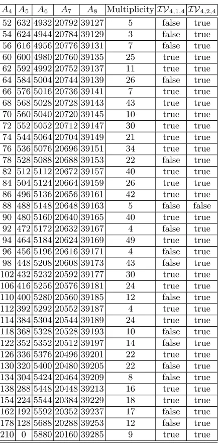
One of the benefits of our classification is that the a-priori huge number of choices for a PRINCE-like linear layer is reduced to a much more manageable amount. This in particular allows to not only focus on the linear and differential branch number, but more detailed one the exact weight distribution of the corresponding additive codes. While this does not improve the (directly) provable bounds on the probabilities of linear and differential trails it has an impact on the number of trails with optimal bias resp. probability. Note that, as proven in [23], the weight distribution of the code and its dual are identical. Moreover, given the number of code-words with minimal weight, the whole weight distribution is fixed (cf. [23, Theorem 4.1]).
Below we give an exhaustive list of the possible weight distributions for all 739 PRINCE-like linear layers.Aidenotes the number of words with weighti. We also give the multiplicity, i.e. how many of the 739 cases lead to the given weight distribution. We furthermore note which of the possible weight distributions occur for linear layers constructed via Theorem 1 either by combiningIV4,1,4 or
IV4,2,4matrices. As can be seen, there is a rather big variance in the number of
code words with minimal weight, ranging from 52 up to 210. While intuitively it seems beneficial to select a code with a minimal number of code words of small weight, the exact benefits of a specific choice depend on cipher details outside the scope of this paper.
D
Security Analysis of
PRIDE
A4 A5 A6 A7 A8 MultiplicityIV4,1,4 IV4,2,4
52 632 4932 20792 39127 5 false true 54 624 4944 20784 39129 3 false true 56 616 4956 20776 39131 7 false true 60 600 4980 20760 39135 25 true true 62 592 4992 20752 39137 11 true true 64 584 5004 20744 39139 26 false true 66 576 5016 20736 39141 7 true true 68 568 5028 20728 39143 43 true true 70 560 5040 20720 39145 10 true true 72 552 5052 20712 39147 30 true true 74 544 5064 20704 39149 21 true true 76 536 5076 20696 39151 34 true true 78 528 5088 20688 39153 22 false true 82 512 5112 20672 39157 40 true true 84 504 5124 20664 39159 26 true true 86 496 5136 20656 39161 42 true true 88 488 5148 20648 39163 5 false false 90 480 5160 20640 39165 40 true true 92 472 5172 20632 39167 4 false true 94 464 5184 20624 39169 49 true true 96 456 5196 20616 39171 4 false true 98 448 5208 20608 39173 43 false true 102 432 5232 20592 39177 30 true true 106 416 5256 20576 39181 24 true true 110 400 5280 20560 39185 12 false true 112 392 5292 20552 39187 4 true true 114 384 5304 20544 39189 24 true true 118 368 5328 20528 39193 10 false true 122 352 5352 20512 39197 14 false true 126 336 5376 20496 39201 22 true true 130 320 5400 20480 39205 22 false true 134 304 5424 20464 39209 8 false true 138 288 5448 20448 39213 16 true true 154 224 5544 20384 39229 18 true true 162 192 5592 20352 39237 17 false true 178 128 5688 20288 39253 12 false true 210 0 5880 20160 39285 9 true true
Fig. 3.The Weight Distribution of All PRINCE-like Codes
We also investigated in detail if there is a significant linear-hull or differential effect.
Here, we justify our assumption of the resistance ofPRIDEagainst classical analysis techniques, such as linear and differential cryptanalysis.
Classical Cryptanalysis. As mentioned above the differential and linear branch numbers ofL0toL3are all 4. Thus, it follows by Theorem 1 that the same holds
for the entire linear layer L. This means we have –at least– 4 active Sboxes per two rounds and thus 32 in 16 rounds. For the Sboxes we selected, the best non-zero differential has probability 1/4. Thus, assuming independent round keys, there is no single differential trail for 16 rounds ofPRIDEwith average proba-bility better than (1/4)32= 2−64, which is too small to be usable for an attack
even when using the full code-book. Similarly, for linear cryptanalysis, we can upper-bound the absolute correlation for any single trail by (1/2)32 = 2−32. Again, this is too small to be of use in an attack.
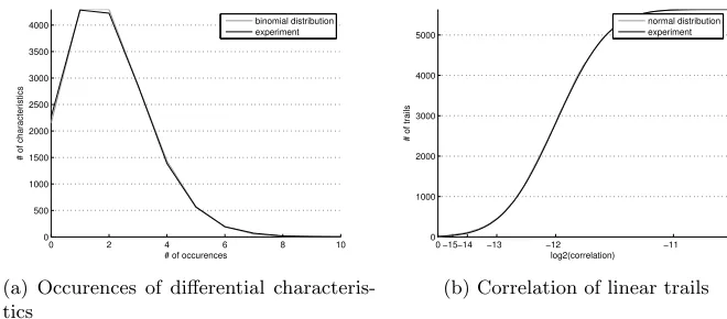
We have computationally generated all optimal characteristics and trails for six rounds of PRIDE. We found 15 871 differentials with probability 2−24 and 5 632 trails with the expected absolute correlation of 2−12. Each optimal char-acteristic (resp. trail) has a unique pair of input and output difference (resp. mask). In other words, there is no clustering of neither optimal characteristics nor optimal trails.
We experimentally verify these results with a round-reduced implementation of the cipher in order to check for linear-hull and differential effects. In the case of differential cryptanalysis, for each input difference we picked a random key and encrypted 225 random plaintexts pairs while counting how often the predicted
output differences were observed. While for some input/output differences the resulting counter was significantly higher than 2, this is not surprising but fits the theory. To illustrate this, Figure 4(a) shows how closely these results match a binomial distribution with parameters
p= 2−24 and N = 225.
In addition, for any characteristic that resulted in a counter above 6 in the previous experiment, we re-run the program with an increased amount of plain-text/ciphertext pairs. Using 230 pairs, no significant differential effect was de-tected.
For the linear part, we performed a similar experiment using 227 plaintexts. Figure 4(b) shows how many (out of the 5 632 trails) resulted in a correlation smaller than a given value. Again, even though some of the observed correla-tions are higher than 2−13, the distribution fits nicely with the theoretically expected normal distribution. Again, we re-ran the experiments for the trails with experimentally high correlation with increased data complexity. No signif-icant linear-hull effect was observed.
0 2 4 6 8 10 0
500 1000 1500 2000 2500 3000 3500 4000
# of occurences
# of characteristics
binomial distribution experiment
(a) Occurences of differential characteris-tics
0 −15−14 −13 −12 −11 0
1000 2000 3000 4000 5000
log2(correlation)
# of trails
normal distribution experiment
(b) Correlation of linear trails
Fig. 4. Experimental results for differential and linear cryptanalysis over six rounds ofPRIDE
found that there is no clustering of those optimal trails/characteristics. Ad-ditionally, our program shows that the bounds we have established are tight. However, PRIDEhas 20 rounds; and in our belief, it should be sufficient.
Other Attacks. We also considered advanced variants of linear and differen-tial attacks. Higher-order differendifferen-tials, truncated differendifferen-tials, impossible differ-entials, and zero-correlation attacks do not seem to pose a threat on PRIDE. It seems that the bit-wise structure of the linear-layer limit the applicability of these attacks.
Finally, we have considered algebraic attacks, but did not find any serious issues.
E
Code Table
The following table contains the best-known (bounds on the) minimal distance for a [2n, n] code over F2b forb= 1,2,3. An entry with a single number means that a code with a minimal distance matching the upper bound exists.
n 2 3 4 5 6 7 8 9 10 11 12 13 14 15 16
F2 2 3 4 4 4 4 5 6 6 7 8 7 8 8 8
F22 3 4 4 5 6 6 7 8 8 8-9 9 10 11 12 11-12