R E S E A R C H
Open Access
Bifurcations in four-dimensional switched
systems
Hany A. Hosham
1,2* *Correspondence:[email protected]; [email protected]
1Department of Mathematics,
Faculty of Science, Taibah University, Yanbu, Saudi Arabia
2Department of Mathematics,
Faculty of Science, Al-Azhar University, Assiut, Egypt
Abstract
In this paper, the focus is on a bifurcation of period-Korbit that can occur in a class of Filippov-type four-dimensional homogenous linear switched systems. We introduce a theoretical framework for analyzing the generalized Poincaré map corresponding to switching manifold. This provides an approach to capturing the possible results concerning the existence of a period-Korbit, stability, a number of invariant cones, and related bifurcation phenomena. Moreover, the analysis identifies criteria for the existence of multi-sliding bifurcation depending on the sensitivity of the system behavior with respect to changes in parameters. Our results show that a period-two orbit involves multi-sliding bifurcation from a period-one orbit. Further, the existence of invariant torus, crossing-sliding, and grazing-sliding bifurcation is investigated. Numerical simulations are carried out to illustrate the results.
Keywords: Period-Korbit; Invariant cones; Sliding motion; Poincaré map; Multi-sliding bifurcation
1 Introduction
Higher dimensional systems (n> 3) are of great significance for applications as modeling problems often require higher dimensions. Therefore, this paper aims to investigate the existence of a period-Korbit, multiple periodic orbits, and related bifurcation in a linear homogeneous switching system which are quite different from those in a smooth system. These phenomena and bifurcation theory are extremely important in understanding the qualitative change in the dynamical behavior that appears on the surface of discontinuity. In smooth systems these topics are especially important phenomena which exist only in the behavior ofnonlinearsystems and are closely related to system stability and may lead to more complicated behavior such as chaos. As an example of the existence of multiple periodic orbits, a subcritical Hopf bifurcation leads to multiple periodic orbits in a stage structured population model [23]. Moreover, in a smooth system the necessary methods have been developed, essentially based on the fact that smooth (differentiable) systems can locally be approximated by linearized systems. Key ingredients developed within that approach are the concepts of invariant manifolds, attractors, and a characterization by characteristic numbers such as Lyapunov exponents. For instance, in the context of bifur-cations of equilibria and stability analysis, center manifold theory is a well-established and mathematically proven procedure to reduce the dimension of dynamical systems.
Switched dynamical system (SDS for short) exhibits a wide variety of complex phenom-ena which cannot be dealt with by the classical theory, but are typically observed in many models of real systems; for instance, stick-slip, chattering, grazing-sliding, and jump phe-nomena were observed in an automotive brake system, impact contact model of a church bell, electronic switches, and genetic networks, respectively. For historical overviews and references, see [3,5,6,10,17,18,22].
In addition, SDS provides a set of possible candidates for motion of transversal cross-ing or attractive slidcross-ing. These systems can exhibit a wide range of nonlinear phe-nomena including either classical bifurcations and chaos or unique phephe-nomena, termed discontinuity-induced bifurcations, that involve the interaction of the systems’ invariant sets with the discontinuity boundaries.
Further, many researchers have used fractional differential equations to develop math-ematical models that appeared in different areas of sciences. In addition, several different control methods have been applied to synchronize the fractional order chaotic systems, for instance, see [8,9]. These results motivated us to combine the fractional differential equations and certain types of discontinuities in vector fields as a future direction of the current work.
Nowadays, there has been growing interest in the fact that the richness of dynamical behavior found in linear SDS covers almost all types of bifurcations found in nonlinear smooth systems such as limit cycles, period-doubling, chaotic transients, homoclinic and heteroclinic, and strange attractors. Furthermore, it has been pointed out that linear SDS can undergo a complex behavior and a great number of completely new bifurcations since the characteristics of these bifurcations depend critically on both the class of SDSs and the geometry of the involved boundaries. Recently, in [12] it was shown that the existence of a novel bifurcation depends sensitively on the location of the return flow. Such an example is the existence of an invariant cone for linear SDS which may exhibit that a periodic orbit will be destroyed suddenly without any change in its stability. Further, in [19] it was shown that the planar linear SDS which has no equilibria in each subsystem, neither real nor virtual, can exhibit at least one limit cycle. For a review of the available results, see [3,4,
6,7,12,14,19,21,27]. According to these researchers, we note that the current results of bifurcation theory for SDS are still incomplete and scarce. What is more, there is no general classification strategy proposed due to the lack of smoothness, suitable methods, and techniques.
transversal crossing and attractive sliding mode. Starting with a piecewise linear system as basic system, it has been shown that the corresponding invariant cones will be deformed to a cone-like surface if higher order terms are added. In that way, we have established a similar reduction procedure to a lower dimensional system for nonlinear SDSs as has been achieved for a smooth system via the center manifold approach.
One method of studying SDS is by constructing a suitable generalized Poincaré map which has several useful properties [16] and then studying its dynamics. Therefore, the existence of invariant cones is equivalent to the existence of positive real eigenvalues of the return Poincaré map.
In this paper, we extend this approach to investigate the existence of the period-Korbit, a number of invariant cones, and associated phenomena. We identify three main challenges associated with finding period-Korbit (i.e., orbits intersecting the surface of discontinuity Ktimes). The first is to find the lowest positive times of intersection with the switching surface that are dependent onξ in a nonlinear way. The second is to construct a Poincaré map analytically, which is not an easy task. The third is to find an eigenvector which forms the period-Korbit.
One further aim of this work is to investigate the existence of multi-sliding, sliding bi-furcation, and dynamics around period-Korbit (i.e., invariant torus). In this situation the trajectories come back to the switching surface several times before close the orbit under the Poincaré map. The main results are formulated in Theorem1.
The contribution of this work is in the theory of discontinuous systems, particularly in the case of Filippov-type flow. More specifically, we obtain crossing-sliding,
grazing-sliding, multiple periodic orbits, invariant cones, and their stability of a class of four-dimensional switched systems. Further, this work provides novel results concerning the existence of a period-K orbit with sliding mode, which is quite different from what is known for a three-dimensional system with single discontinuity surface.
Let us start with a simple example in order to show that the basic reason for the existence of period-doubling bifurcation is the presence of certain types of nonlinearities in SDS.
2 Model of the vibration system excited by a harmonic force
We consider a simple vibration system of a single-degree-of-freedom oscillator with a bi-linear restoring force [22]. When the system is externally excited by a harmonic force, the equation of motion may be written as follows:
¨
x+ 2αx˙+x=βcos(wt), forx≤x0,
¨
x+ 2αx˙+w¯2+1 –w¯2x0=βcos(wt), forx≥x0.
(1)
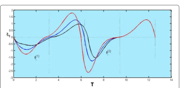
Figure 1Transition of a period-one orbit to period-two orbits in nonlinear system (2) periodT into an orbit with period 2T. In this model the bifurcation parameter is taken asωand the other parameters are fixed asw¯ = 4,α= 0.125. The numerical simulation illustrates that the bifurcation actually occurs betweenw= 2.40 andw= 2.42. Figure1
shows the transition of a period-one orbit to period-two orbits. This transition is called periodic doubling bifurcation which occurs due to the presence of nonlinear harmonic force.
In the next section we introduce a class of four-dimensional homogenous linear SDSs with two-zone and provide a methodology to ensure that the system has a period-Korbit.
3 The existence of a period-Korbit in SDS
3.1 Setting of the problem
We start our investigations by considering a four-dimensional homogenous linear SDS for which the evolution of a variableξ in some region is determined by the equations
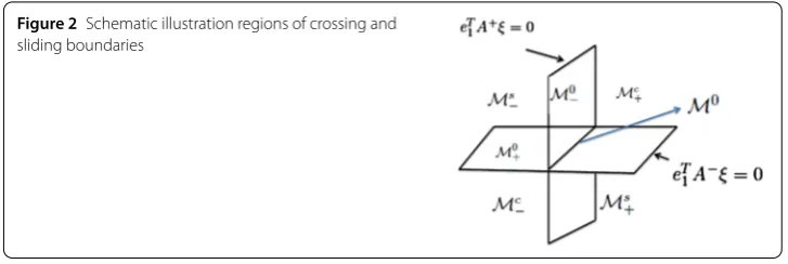
Figure 2Schematic illustration regions of crossing and sliding boundaries
M. Hence, the both sets of crossing regions (see Fig. 2) are given by Mc–={ξ ∈M| ξ2>μ(β–ξ3+ (α––λ–)ξ4) > 0}andMc+={ξ ∈M|ξ2<μ(β–ξ3+ (α––λ–)ξ4) < 0}. The sliding regions are given by Ms
–={ξ ∈M|0 <ξ2<μ(β–ξ3+ (α––λ–)ξ4)} andMs+=
{ξ∈M|0 >ξ2>μ(β–ξ3+ (α––λ–)ξ4)}, whereMs–is called attractive sliding mode and Ms
+ is called repulsive sliding mode. Further,M0–={ξ ∈M|ξ2=μ(β–ξ3+ (α––λ–)ξ4}, M0
+={ξ ∈M|ξ2= 0}define the boundaries between sliding and crossing modes, and M0=M0
–∩M0+defines the intersection plane between two boundaries.
The flow in Ms itself is governed by Filippov’s extension as follows:ξ˙=qA+ξ + (1 –
q)A–ξ,q∈[0, 1], whereq(ξ) = eT1A–ξ
eT1(A––A+)ξ andA±is a Jacobian linearization of (3).
There-fore, we have an explicit form of the sliding vector field
˙
ξ=A+ξ– e
T
1A+ξ
eT1(A––A+)ξ
A––A+ξ. (4)
This sliding system becomes a linear system if and only if there exist vectorsx,y∈R4such that (A+–A–)(I–e
1eT1) =xyTholds (see Theorem 5.3 in [18]). The choice of matrices in (3) is taken in a more general form such that system (3) exhibits a rich variety of bifurcation behaviors depending on different parameters. Thus, without loss of generality, assume that
A±=S±–1A±NS±, S–=e1,e2,e3,μ(e1+e4/μ)
,
S+=I, A±N=
⎛ ⎜ ⎜ ⎜ ⎝
λ± –1 0 0
1 λ± 0 0
0 0 α± –β±
0 0 β± α±
⎞ ⎟ ⎟ ⎟ ⎠.
(5)
The following lemma collects several useful properties of (3).
Lemma 1 For system(3),the following properties hold:
• Eigenvalues ofA±areλ±±iandα±±iβ±(withλ±,α±,β±∈R,β±> 0). • The origin is the only equilibrium point in each sub-system.
• The⊕-system possesses an invariant planeeT
3ξ=eT4ξ= 0with constant return time
t+(ξ) =π.
• For the-system,the surface generated byξ2=β–μξ3+μ(α––λ–)ξ4determines the boundary of the sliding motion area in the(ξ2,ξ3,ξ4)-phase space.
• The intersection times(hit times)are constants on rays in all regions.
• Ifξ∈M0,thenξ is called a two-fold singularity or the Filippov system has a singular point.
Proof By direct calculation of eigenvalues ofA±, we haveλ±±iandα±±iβ±,β±> 0, and sinceA±are nonsingular matrices, then the origin is the only equilibrium point. For the
⊕-system, we haveMc
–={ξ ∈M|ξ2> 0},Mc+={ξ ∈M|ξ2< 0}; hence, the intersection timet+(ξ) =π is constant and, by means of vector field evaluation at M, we findξ2=
β–μξ3+μ(α––λ–)ξ4determines the boundary of the sliding motion area. In addition, let
λ+=λ–,α+=α–,β±= 0 in (4), the sliding flow becomes linear.
Further, whenμ= 0, we findMs:={φ}, which means that there is no sliding motion
area. Furthermore, the intersection times (hit times) are constants on rays in all regions due to the homogeneity of system (3) (see [16]). Last, ifξ∈M0, we findeT
1A–ξ=eT1A+ξ= 0
in (4), and therefore the Filippov system has a singular point.
Note that transformation (5) does not perturb the switching manifoldM. Then the general solution of (3) is given by
ψ(t±,ξ) =eλ±t±cos(t±)S±–1e
1+sin(t±)S±–1e2
¯ ξ1
+cos(t±)S±–1e2–sin(t±)S±–1e1
¯ ξ2
×eα±t±cosβ±t±S±–1e3+sin
β±t±S±–1e4
¯ ξ3
+cosβ±t±S±–1e4–sin
β±t±S±–1e3
¯ ξ4
,
(6)
where
S±ξ(0) =ξ¯, ξ(0) =0,ξ20,ξ30,ξ30T∈Mc.
The general solution (6) allows us to construct Poincaré mapsP±for⊕and-systems, respectively. The flow starts from the initial pointξ0∈Mc–and spends a timet–before it returns to ψ(t–,ξ)∈Mc+, then we can define the map P–(ξ) :=Mc–→Mc+. At that point, the flow starts once again and spends a timet+ before it reachesψ(t+,ξ)∈Mc–, we can define the mapP+(ξ) :=Mc+→Mc–. The return timest±(ξ) depend onξ and are determined as the lowest positive root ofeT
1ψ±(t±,ξ) = 0. If the flow of a subsystem of (3) arrives at the attractive sliding regionMs
–, the sliding flow can be observed along a three-dimensional discontinuity surface, whereξ∈Ms, and lettsbe the time spent inMs. Then
we define the sliding map asPs:=Ms
–→Ms–.
From a local point of view, a generalized Poincaré map can be thought of as a compo-sition of sub-maps (P–,P+,Ps). Further, if the trajectories of (3) come back toMseveral times before close the orbit, thenPK represents the composition ofPwith itself or sub-mapsKtimes.
Lemma 2 Consider a generalized Poincaré mapping PK(where PKis theKth iterate of P)
structure for period-Korbit either without sliding mode
PK(ξ) = (Pi◦Pj)K(ξ) =ξ, i,j∈ {+, –},i=j,K> 1,
or with sliding mode
PK(ξ) = (Pi◦Pk◦Pj)K(ξ) =ξ, i,j,k∈ {+, –,s},i=j=k,K> 1,
PK–1(ξ)=ξ,
such that tK–,t+K,tsKexist.Then SDS(3)has a period-Korbit without or with sliding mode,
respectively.
Proof We assume that the local Poincaré section isMand the time functionstK±,tsKexist. By using the fact that a periodic point of the full system (3) with crossing the Poincarè sectionKtimes is a fixed point of thePKiterate ofP, by cyclic invariance, SDS (3) has a
period-Korbit without or with sliding mode.
The existence of invariant cones for (3) depends on the existence of a positive eigenvalue of the generalized Poincaré map (i.e.,PK(ξ) =μcξ,μc> 0). This leads to the fact that the
existence of a period-Korbit is just a sufficient condition for the existence of invariant cone foliated by orbits.
3.2 Main results
The main results focus on the classification of the possible bifurcation scenarios that can occur in (3) and are summarized in the following theorem. This theorem provides a general framework and conditions in which the existence of period-Korbit, stability, a number of invariant cones, multi-sliding bifurcation, invariant torus, and crossing or grazing-sliding bifurcation in system (3) take place. These results are carried out by using the characterization of a generalized Poincaré map.
Theorem 1 For the linear SDS(3),the following statements hold:
(I) Suppose the caseλ+= –λ–.Then:
1. The system has a flat periodic orbit(degenerate situation)contained with the invariant plane(ξ¯1,ξ¯2)andt–=π.
2. Assume also thatα–=λ–= –λ+= –α+,β–+β+=K∈Z,to characterize complex behaviors.
2.1 Whenξ¯∈Mc–andξ¯2>μβ–ξ¯3.Then the system has a family of period-one orbits with periodT= 2πifKis even and a family of
period-two orbits with periodT= 4πifKis odd such thatβ+is even(i.e., β–is odd).Further,ifβ+is odd(i.e.,β–is even),then the system has three families of period-two orbits.
2.2 Whenξ¯∈M0
–andξ¯2=μβ–ξ¯3.Then the system has two families of period-one orbits with a segment of sliding motion ifKis even,and these orbits can also undergo a grazing-sliding bifurcation.As well there is a transition from period-one orbit to period-two orbit with two segments of sliding motion(multi-sliding)ifKis odd.
(II) Assume thatξ¯∈M0–,σ= (α––λ–) < 0.Then:
sliding periodic boundary surface under the Poincaré map is satisfied:
β–sint––eσt–sinβt–
σsint–+cost––eσt–cosβ–t–
= β
–(eλ+π+λ–t–cos(t
–) + 1)
eλ+π+λ–t–
(σcos(t–) –sint–) +σ = 0.
2. The system has a family of period-one orbits generated byξ¯∈M0–with
t–∈(π, 2π)andβ±= 0if and only if
eλ+π+λ–t–σcos(t–) –sint
–
+σ= 0.
3. The system has a family of period-one orbits with sliding mode which is generated byξ¯∈M0–witht–∈(π, 2π)andβ±= 0if and only if
eT1P–(ξ¯) <μσeT3P–(ξ¯) < 0, 0 <eT1P(ξ¯) <μσeT3P(ξ¯).
Moreover,the system undergoes the crossing-sliding bifurcation due to the transition between crossing and sliding modes.
(III) Assume thatσ= 0andλ+= –λ–.Then:
1. There is a family of flat periodic orbits generated by the invariant (ξ¯1,ξ¯2)-plane with periodT= 2π.
2. There are two families of period-two orbits ifβ–= 1,α+= –α–,one of them is generated by the boundary surface of sliding region with period
T= 2π+3i=1t(i)
– and the other is generated by any vectorξ¯∈Mc–with periodT= 4π.
3. There are two families of period-one orbits ifβ–= 2,α+= –α–,one of them is generated byξ¯={¯ξ∈M0–|¯ξ4= 0}with periodT= 2πand the other is generatedξ¯={¯ξ∈Mc–|¯ξ4= 0}with periodT= 2π.
(IV) Suppose thatμ= 0(i.e.,Ms=∅)andα+= –α–.Then:
1. The system has two families of period-one orbits,one of them is generated by the invariant(ξ¯1,ξ¯2)-plane with periodT= 2πand the other is generated by any vectorξ¯∈Msuch thatβ–+β+=Kis even withT= 2πifλ+= –λ–. Further,there is a transition from period-one orbit to period- two orbit ifKis odd.
2. The system has a family of period-Korbits or an invariant torus if and only if
Kis an irrational number.
with single discontinuity surface. Further, in such cases we observe a sudden transition through the discontinuity manifold.
3.3 Construction of the generalized Poincaré map
For rigorous evaluation of the generalized Poincaré map, we use analytical formulas for trajectories of system (3), which are given by (6). The Poincaré mapP–(ξ) :=Mc–→Mc+
Note that the return timet–(ξ) depends onξ in a nonlinear way, and it is actually the first one possible inMc
–. It means that the trajectory of-system intersectsMtransversally if we can find the smallest positive root of the following equation:
Ft–(ξ)
The second iterate of the generalized Poincaré return map is given as follows:
E= –μe2λ+π+λ–(t(1)– +t(2)– )cost(2)
The second return timest–(2)is given as the smallest positive root of the following equation:
F2
In the same way, we can getKiterate of the Poincaré map.
Lemma 3 We assume thatξ¯ is a fixed point of the generalized Poincaré map P(ξ¯) =ξ¯or P2(ξ¯) =ξ¯,respectively.If all eigenvalues of linearized P(resp.P2))atξ¯satisfy|μ
c|< 1 (resp. | ˆμc|< 1),thenξ¯is asymptotically stable,and if|μc|> 1 (resp.| ˆμc|> 1),thenξ¯is unstable. If|μc|= 1 (resp.| ˆμc|= 1),thenξ¯generates a periodic behavior.
IfK= 2,the eigenvalues of the linearized Poincaré map(8)and(9),respectively,are given as: existence of periodic behavior and stability of system (3). Now, we are ready to prove all items of Theorem1, respectively.
3.4 Proof of the main results
(I) Becauseξ¯∈Mc
–, then the resultξ¯2>μβ–ξ¯3directly follows from the definition of the crossing regionMc
–. Letμ1c= 1 corresponding to a period-one orbit of the Poincaré map
(8). Then we get one possible solutionλ–= –λ+ andt
–=π that must be verified by the nonlinear equation (7). Hence, we get
F(π) = –μξ4–μe(α
= –1, which is not possible. Moreover, regarding Lemma2, the corresponding eigenvector, which is responsible for generating a period-one orbit, requires eitherξ3=
ξ4= 0 orξ3= 0,ξ4= 0.
(a) Ifξ3=ξ4= 0is invariant surface, then we obtain a flat period-one orbit contained
with the invariant plane(ξ¯1,ξ¯2), which is a trivial situation for our purposes.
(b) Ifξ3= 0,ξ4= 0lead toα–= –α+andβ–+β+=K∈Zis even. Therefore we get a
On the other hand, the existence of a period-two orbit is associated with an eigenvalue of the Jacobian of the Poincaré map (8) equal –1 andP2(ξ¯) =ξ¯ (Lemma3). Then, when
α–=λ–= –λ+= –α+, we find that the positive rootst(1)
– =t–(2)=πsatisfy equations (7) and (10) if and only ifβ–is odd whereβ–+β+=K∈Zis odd (i.e.,β+is even). For instance, see Fig.3(b), (c).
Ifβ–is even (i.e.,β+is odd), the three families of period-two orbits are made up for by compensatory changes in the time spent in the-system. Hence, we compute the pos-sible intersection times under attraction of PK. Then there are three cases of existence of the intersections times that are given by (7) and (10); ift(1)
– =t–(2)=π, so there are two possibilities, namely eithert–(1)∈(0,π),t–(2)∈(π, 2π) ort–(2)∈(0,π),t–(1)∈(π, 2π), and we findξ¯∈Mc–is a fixed point ofP2(ξ¯). Further, ift(1)
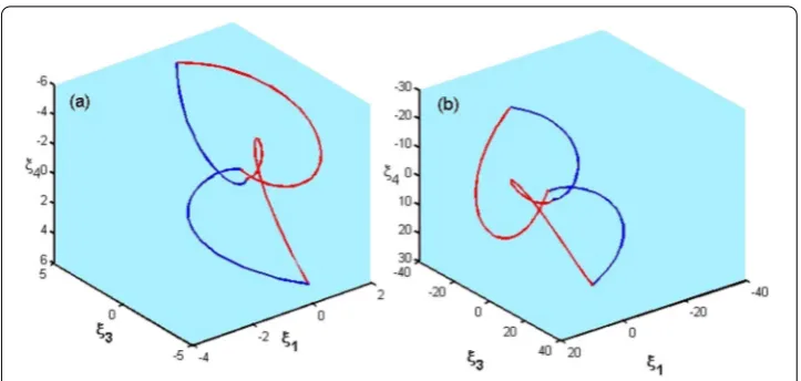
– =t–(2)=π, thenξ¯={¯ξ∈Mc–|¯ξ4= 0}is a fixed point ofP2(ξ¯). The commutative parameters have no effect on the stability of period-two orbits but are introduced as a perturbation of switching times. Figure4illustrates the existence of three different switching times, which leads to the existence of three families of period-two orbits.
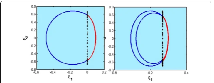
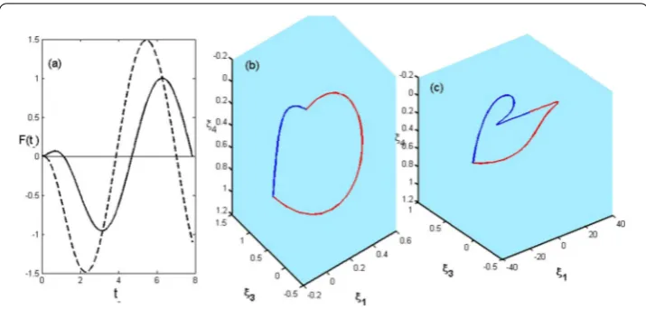
Figure 3(a) Nontrivial period-one orbit whenβ–=β+= –α–= 1 (Kis even). (b), (c) Period-two orbits when β–= 0.5β+= –α–= 1 (Kis odd)
The sliding trajectories (4) occur on the discontinuous three-dimensional surfaceMs.
Subsequently, system (4) can be rewritten in the reduced form as follows:
˙
Then one can easily getPsto understand the behavior of the trajectory atM0–.
The nongeneric bifurcation of limit cycles occurs when the sliding flow becomes tan-gent to the surface of discontinuity; hence, the tangency points play an important role precisely when the flow passes through one of these points. Further, three situations may occur when a solution starts or reachesM0–: (a) the trajectory will be forced to leaveM0– to enterMc
–if (eT1A–.A–ξ)|ξ¯ < 0; (b) the trajectory entersMs–if (eT1A–.A–ξ)|ξ¯> 0; (c) the trajectory remains (local minimum) onM0
–if (eT1A–.A–ξ)|ξ¯ = 0 with several future possi-bilities depending on high time derivatives ofq(ξ) along the flow onM0
–. For our system odic orbit with a segment of sliding motion in the phase space. Moreover, depending on bifurcation parameterβ+, our system can exhibit complex bifurcation scenarios by fixing
β+= 1 (i.e.,K= 3). There is a transition from period-one orbit to period-two orbits with two segments of sliding motion. This transition depends on the sensitivity of the system behavior with respect to changes in parameters, and it is called multi-sliding bifurcation, see Fig.6. Whereas in the other situation whenβ–= 1, the existence of period-one or-bit with a segment of sliding motion can also occur if the trajectory is forced to leave negative regionM0
– (i.e.,ξ¯ ={¯ξ∈M–0|¯ξ2< 0}and enterMc+. In this case we note that
β+= 1,eT
1A–.A–ξ¯= 0,eT1A+.A+ξ¯> 0); therefore the Poincaré mapP(ξ¯) =PsP+(ξ¯) has a fixed
character-Figure 5Period-one orbit with a segment of sliding motion established byξ¯∈M0
–. (a), (b) Ifξ¯4= 0,β–= 2.
(c) Ifξ¯4= 0,β–= 1, the flow has no intersection withMc, which is called one-zonal orbit
Figure 6Period-two orbit with a segment of sliding motion established byξ¯∈M0
–whenξ¯4= 0,β–= 2, K= 3
ized by a trajectory of the⊕-system that becomes tangent toM. Strictly speaking, there is a set of points that does not interact withMand a set of points that hitsM. Therefore, by varying parameters, the sliding segment becomes an infinitesimally small sliding segment that is close to a grazing bifurcation point.
(II) Ifξ∈M0
–andσ< 0 imply that the trajectory entersMc–. Using (7) and without loss of generality, we assume that ξ4
ξ3 = 1, we get
F(β–,σ)(t–) =β–sint––eσt–sinβ–t–+σsint–+cost––eσt–cosβ–t–= 0. (14)
It can be seen thatF(β–,σ)(t–) =F(–β–,–σ)(–t–) for any (β–,σ,t–)∈R. Furthermore, we get F(β–,σ)(0) =F
(β–,σ)(0) = 0, and whereσ < 0, we getF(β–,σ)(π) < 0,F
(β–,σ)(0) = (β–)2– 1 – σ(σ+ 2β–). Thent–∈(0,π) ifF
Figure 7(a) The behavior of equation (14) for different values ofσ. (b), (c) Short and long time periods (t–= 1.6954,t–= 3.7296), respectively
t–∈(π, 2π). In Fig.7(a), the first positive solution of (14) ist–∈(0,π) whenσ= –1 (solid curve) and becomest–∈(π, 2π) whenσ= –2.1 (dashed curve).
Letμ2
c = 1 corresponding to a period-one orbit of the Poincaré map (8). Then we get
one possible solutionβ+= (2π–β–t–)/πandt –= –α
+
α–π. Hence,T= (1 –α +
α–)π, α +
α– < 0.
Becauseξ¯∈M0
–, which means that we have specified a value ofξ¯2=μβ–ξ¯3+μσξ¯4> 0, hence, we will get the image of the lineξ40=m0ξ30 via a slope transition mapS:R→R,
m1=S(m0), wherem1= ξ41
ξ31 passes through (ξ 1
3,ξ41) =P(ξ30,ξ40). Then system (3) has a family of periodic orbits which is generated byP(ξ¯) =ξ¯if and only ifm1=m0(whereξ1=ξ0), then we get
β–sint––eσt–sinβ–t–
σsint–+cost––eσt–cosβ–t–
= β
–(eλ+π+λ–t–cos(t–) + 1) eλ+π+λ–t–
(σcos(t–) –sint–) +σ.
This proves item 1. in (II). For example, we assume that σ= –0.5, β–=μ= 1, then by the above result we getλ+= 0.3022,α+= 0.8095, andβ+= 1.4603 with short periodT= 1.5397π, see Fig.7(b). Further, if we change the parameterσ = –2.5, then we getλ+= –1.2457,α+= 1.7808,β+= 0.8128,μ= –1 with long periodT= 2.1872π, see Fig.7(c).
2. Ifβ±= 0, then equation (14) becomes
F(0,σ)(t–) =σsint–+cost––eσt–= 0. (15)
We can easily investigate the global behavior of solutions to (15). Then we gett–∈(π, 2π) ifσ< 0. It should be pointed out here that ifσ> 0, then the trajectory leavesM0–to enter Mc
–, but it cannot leaveMc–for all future times. Hence there is no finite return time, and thus the existence of a close orbit is impossible.
Letμ(2)c = 1 corresponding to a period-one orbit of the Poincaré map (8). Then we get t–= –α
+
α–π. Hence,T= (1 –α +
α–)π, α +
α– < 0. Further, the fixed point equationP(ξ¯) =ξ¯ holds
ifeλ+π+λ–t
–(σcos(t–) –sint–) +σ= 0.
3. As we know from 2., the intersection timet–is uniquely determined ast–∈(π, 2π) ifσ< 0. The trajectory after reachingMc
+switches to the⊕-system. This flow starting in Mc
flow leavesMto enter the attractive sliding modeMs
–, via Poincaré maps (P–andP) and according to the definition of crossing and sliding modes, we get the necessary conditions:
eT1P–(ξ¯) <μσeT3P–(ξ¯) < 0, 0 <eT1P(ξ¯) <μσeT3P(ξ¯).
For example, we fix the parameter σ = –0.1, then t– = 5.2420,α+ = –0.1669, and at
λ+= –1, we show that the period-one orbit hits tangentially the boundary of the sliding regionM0
–with zero time (i.e.,ts= 0). The crossing-sliding bifurcation can be observed
by varying just one control parameterλ+, where the system possesses a period-one orbit with a segment of sliding motion (ts= 0.11) ifλ+= –1.322.
Next we fixσ= 0,λ+= –λ–and we prove that system (3) has different families of period one or two orbits.
(III) Ifσ= 0, then equation (7) reduces to
F(β–)(t–) =sint–ξ2–μsinβ–t–ξ3+μcost––cosβ–t–ξ4= 0. (16)
1. Ifλ+= –λ–,t–=π, then system (3) has a single family of flat periodic orbits. To see
this, note thatP(ξ) =ξyieldsξ3=ξ4= 0and equation (7) is satisfied for allβ–∈R.
2. To prove the existence of two families of period-two orbits, we investigate the Poincaré map which brings the pointξback to itself after some iteration of sub-maps.
If we fixβ–= 1 andα+= –α–, equation (7) reduces to
Ft(1)– =sint–(1)(ξ2–μξ3) = 0. (17)
Then there are two solutions, namely eitherξ2–μξ3= 0, which means thatξ∈M0–with
t(1)
– =π, orξ∈Mc–witht–(1)=π, respectively.
Firstly, we consider the situation thatξ∈M0–andt(1)– =π.
In this case, we consider the mapP(ξ) =P–(P2(ξ)) which generates a family of period-two orbits starting with boundary of sliding surface. BecauseP2(ξ) is given by (9), then we getP(ξ) as follows:
P(ξ) =eα–t(3)– ⎛ ⎜ ⎝
Bcost(3)
– Dcost(3)– –μSsint–(3) Ecost(3)– –μCsint(3)–
0 Ccost(3)
– –Ssint–(3) –Scost–(3)–Csint(3)– 0 Scost–(3)+Csint–(3) Ccost–(3)–Ssint–(3)
⎞ ⎟ ⎠
⎛ ⎜ ⎝ ξ2
ξ3
ξ4
⎞ ⎟ ⎠.
(18)
Further, the second intersection time for the-system is given by (10) which is reduced to
Ft(2)– =sint–(2)eT1P(ξ) –μeT2P(ξ)= 0. (19)
Then there is only one solution t(2)– =π where eT1P(ξ) –μeT2P(ξ)= 0 due to P(ξ)=ξ (Lemma2), hence we getD= 0 in (18).
We now scrutinize the geometry of iterations of the Poincaré map. In this situation we have consideredM0
–as a Poincaré surface, thenP(ξ),P2(ξ), andP(ξ) return toM0–again such thatP(ξ)=ξ,P2(ξ)= ξ, andP(ξ) =ξ, respectively. BecauseP(ξ)∈M0
Figure 8Period-two orbit established by: (a)ξ¯∈M0
–the invariant surface of boundary of sliding mode,
(b)ξ¯∈Mc
–which is any point in the crossing region
then we geteT
1P(ξ) > 0 andeT1P2(ξ) > 0, which results incos(t–(1)) = 0, hencet(1)– =π2. Then we findB=C= 0 and the Poincaré map (18) takes the form
P(ξ) =eα–t(3)– ⎛ ⎜ ⎝
0 –μSsint(3)
– Ecost(3)– 0 –Ssint(3)
– –Scost–(3) 0 Scost(3)– –Ssint–(3) ⎞ ⎟ ⎠
⎛ ⎜ ⎝ ξ2
ξ3
ξ4
⎞ ⎟ ⎠.
In addition,P(ξ¯) =ξ¯is satisfied, which requires thateT
1P(ξ) –μeT2P(ξ) = 0. Then we get 2eα–(t(3)– –π2)cos(t(3)
– )ξ4= 0, whereξ4= 0, thent–(3)=π2.
An example to illustrate this situation is shown in Fig.8(a) with parameters valuesβ–=
α+= –α–=λ+= –λ–= 1.
Secondly, we consider the situation thatξ∈Mc–andt(1)
– =π. The intersection timet–(2), which is given by (10), can be rewritten as follows:
Ft(2)– =sint–(2)(ξ2+μξ3) = 0. (20)
Then there is only one solution t(2)
– =π, whereξ ∈/ M–0 andP(ξ)=ξ. Further, we find thatP2(ξ) =ξholds for our fixed parameters. Figure8(b) shows that a period-two orbit is generated by any point in the crossing regionξ¯∈Mc
–, with the same parameter values as in Fig.8(a).
3. Ifξ¯={¯ξ∈M–0|¯ξ4= 0}orξ¯={¯ξ∈Mc–|¯ξ4= 0}andβ–= 2, then equation (7) becomes
Ft(1)– =sint–(1)ξ2– 2μcost–(1)ξ3
= 0. (21)
Therefore we have two possibilities: (a)sint(1)
– = 0 (i.e.,t(1)– =π), or (b)ξ2– 2μcost–(1)ξ3= 0. For case (a) the fixed point equationP(ξ¯) =ξ¯is required to fixα+= –α–andβ+is an even number.
For case (b) whereξ¯∈M0
–(i.e.,ξ2– 2μξ3= 0), it is not possible to findξ2– 2μcost(1)– ξ3= 0 ift(1)
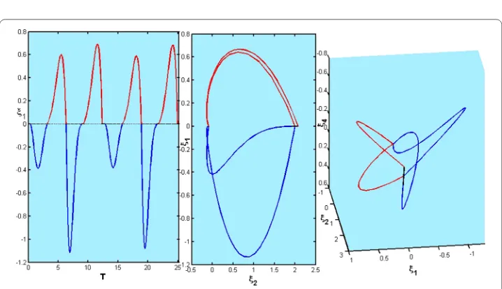
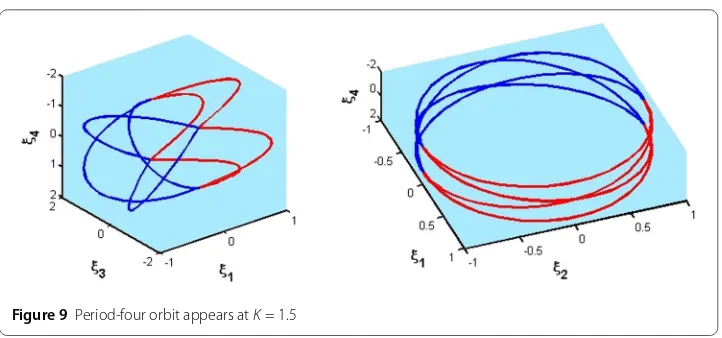
Figure 9Period-four orbit appears atK= 1.5
case (a), and it is not possible to consider case (b) in view of our choice of parametrization of the periodic orbits.
(IV) Ifμ= 0 (i.e.,Ms=∅).
1. As a result of direct observation, we gett(1)
– =πwhereξ¯2= 0. Further, via
investigating the first return map, we find one family of flat period-one orbits if λ+= –λ–andξ¯3=ξ¯4= 0.
On the other hand, ifξ¯∈Mc–andα+= –α–, then it is easy to show that system (3) has a family of period-one orbits ifKis even and the transition from a period-one orbit to period-two orbits ifKis odd wheret(2)
– =π. This proves item 1. in (IV).
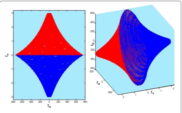
2. Because the eigenvalues of linearizedPhave a complex form (Lemma3), then an invariant torus can occur when a complex-conjugate pair of eigenvalues with unit modulus crosses the unit circle at an angle that is irrational ofπ. The presence of a complex pair of eigenvalues within the unit circle means that the stable fixed point (spiral in) of the generalized Poincaré map becomes unstable (spiral out) and close invariant torus arises around the fixed point (this situation is equivalent to Neimark–Sacker bifurcation). If there are noKiterations ofPKbringing the trajectory back to the same point on the curve, then it produces a quasi-periodic orbit. We considerKto be a control parameter and fix all other parameters in the most simple situation. Then a period-four orbit exists ifK= 1.5, see Fig.9. Moreover, ifK= 1.51, an invariant torus arises, see Fig.10. Another example of a bifurcation is when a control parameterKis changed. We fix the parameters α–= –α+= 2,λ–= –λ+= 0.01. Then system (3) exhibits a period-one orbit when K= 24, and there is a transition to period-two orbit, period-five orbit, and invariant torus whenK= 25,K= 24.4, andK= 24.4321, respectively (see Figs.11and12).
4 Conclusion
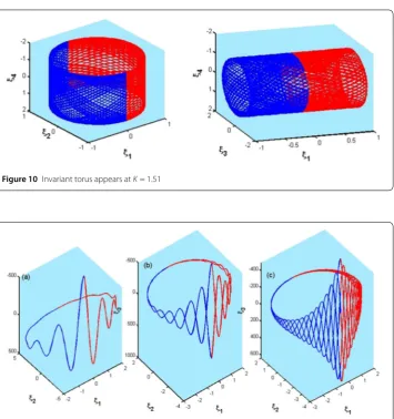
Figure 10 Invariant torus appears atK= 1.51
Figure 11 Transition from period-one orbit to period-two orbit and period-five orbit due to varying ofK= 24,
K= 25, andK= 24.4, respectively
In the forthcoming work, we will consider the situation that the boundaries of the sliding region intersect transversally, whereξ∈M0is a two-fold singularity (see Lemma1and Fig.2). This can have a dramatic effect, and we will give a classification of the existence of invariant cones nearby.
Figure 12 Invariant torus appears atK= 24.4321
Acknowledgements
The author is thankful to the reviewers for their useful corrections and suggestions, which improved the quality of this paper.
Funding
Not applicable. (No funding was received.)
Availability of data and materials Not applicable.
Competing interests
I declare that I have no significant competing financial, professional, or personal interests that might have influenced the performance or presentation of the work described in this manuscript.
Authors’ contributions
The author read and approved the final manuscript.
Publisher’s Note
Springer Nature remains neutral with regard to jurisdictional claims in published maps and institutional affiliations.
Received: 5 September 2018 Accepted: 15 October 2018
References
1. Alipour, M., Arshad, S., Baleanu, D.: Numerical and bifurcations analysis for multi-order fractional model of HIV infection of CD4 T-cells. UPB Sci. Bull., Ser. A78(4), 243–258 (2016)
2. Babakhani, A., Baleanu, D., Khanbabaie, R.: Hopf bifurcation for a class of fractional differential equations with delay. Nonlinear Dyn.69(3), 101–116 (2012)
3. Brogliato, B.: Nonsmooth Mechanics – Models, Dynamics and Control. Springer, London (1999)
4. Carmona, V., Fernández-García, S., Freire, E.: Saddle-node bifurcation of invariant cones in 3d piecewise linear systems. Phys. D: Nonlinear Phenom.241, 623–635 (2012)
5. di Bernardo, M., Budd, C., Champneys, A.R., Kowalczyk, P.: Piecewise-Smooth Dynamical Systems: Theory and Applications. Applied Mathematics Series, vol. 163. Springer, London (2008)
6. di Bernardo, M., Budd, C., Champneys, A.R., Kowalczyk, P., Nordmark, A.B., Olivar, G., Piiroinen, P.T.: Bifurcations in nonsmooth dynamical systems. SIAM Rev.50(4), 629–701 (2008)
7. Feˇckan, M., Pospísil, M.: Poincaré–Andronov–Melnikov Analysis for Non-smooth Systems. Academic Press is an imprint of Elsevier, London (2016)
8. Golmankhaneh, A.K., Arefi, R., Baleanu, D.: The proposed modified Liu system with fractional order. Adv. Math. Phys.
2013, Article ID 186037 (2013)
9. Golmankhaneh, A.K., Arefi, R., Baleanu, D.: Synchronization in a nonidentical fractional order of a proposed modified system. J. Vib. Control21(6), 1154–1161 (2015)
11. Hajipour, M., Jajarmi, A., Baleanu, D.: An efficient non-standard finite difference scheme for a class of fractional chaotic systems. J. Comput. Nonlinear Dyn.13(2), 021013 (2017)
12. Hosham, H.A.: Bifurcation of periodic orbits in discontinuous systems. Nonlinear Dyn.87(1), 135–148 (2017) 13. Huan, S.M.: Existence and stability of invariant cones in 3-dim homogeneous piecewise linear systems with two
zones. Int. J. Bifurc. Chaos27(1), 1750007 (2017)
14. Huan, S.M., Yang, X.S.: Existence of chaotic invariant set in a class of 4-dimensional piecewise linear dynamical systems. Int. J. Bifurc. Chaos24(12), 1450158 (2014)
15. Küpper, T.: Invariant cones for non-smooth systems. Math. Comput. Simul.79, 1396–1409 (2008)
16. Küpper, T., Hosham, H.A.: Reduction to invariant cones for non-smooth systems. Math. Comput. Simul.81, 980–995 (2011)
17. Küpper, T., Hosham, H.A., Dudtschenko, K.: The dynamics of bells as impacting system. J. Mech. Eng. Sci.225(10), 2436–2443 (2011)
18. Küpper, T., Hosham, H.A., Weiss, D.: Bifurcation for nonsmooth dynamical systems via reduction methods. In: Johann, A., Kruse, H.-P., Rupp, F., Schmitz, S. (eds.) Recent Trends in Dynamical Systems. Proceedings in Mathematics and Statistics, vol. 35, pp. 79–105. Springer, Basel (2013)
19. Llibre, J., Teixeira, M.A.: Piecewise linear differential systems without equilibria produce limit cycles? Nonlinear Dyn.
88(1), 157–164 (2017)
20. Li, L., Wang, Z., Li, Y., Lu, J., Shen, H.: Hopf bifurcation analysis of a complex-valued neural network model with discrete and distributed delays. Appl. Math. Comput.330, 152–169 (2018)
21. Makarenkov, O., Lamb, J.S.W.: Dynamics and bifurcations of nonsmooth systems: a survey. Phys. D: Nonlinear Phenom.241, 1826–1844 (2012)
22. Shaw, S.W., Holmes, P.J.: A periodically forced piecewise linear oscillator. J. Sound Vib.90, 129–155 (1983) 23. Thieme, H.R.: Mathematics in Population Biology. Princeton University Press, Princeton (2003)
24. Wang, Z., Wang, X., Li, Y., Huang, X.: Stability and Hopf bifurcation of fractional-order complex-valued single neuron model with time delay. Int. J. Bifurc. Chaos27(13), 1750209 (2017)
25. Weiss, D., Küpper, T., Hosham, H.A.: Invariant manifolds for nonsmooth systems. Phys. D: Nonlinear Phenom.241(22), 1895–1902 (2012)
26. Weiss, D., Küpper, T., Hosham, H.A.: Invariant manifolds for nonsmooth systems with sliding mode. Math. Comput. Simul.110, 15–32 (2015)