An optimized finite difference Crank Nicolson iterative scheme for the 2D Sobolev equation

R E S E A R C H

Open Access

An optimized finite difference

Crank-Nicolson iterative scheme for the 2D

Sobolev equation

Hong Xia

_{and Zhendong Luo}

*_{Correspondence: [email protected]}

2_{School of Mathematics and}

Physics, North China Electric Power University, No. 2, Bei Nong Road, Changping District, Beijing, 102206, China

Full list of author information is available at the end of the article

Abstract

In this paper, we devote ourselves to establishing the unconditionally stable and absolutely convergent optimized finite difference Crank-Nicolson iterative (OFDCNI) scheme containing very few degrees of freedom but holding sufficiently high accuracy for the two-dimensional (2D) Sobolev equation by means of the proper orthogonal decomposition (POD) technique, analyzing the stability and convergence of the OFDCNI solutions and using the numerical simulations to verify the feasibility and effectiveness of the OFDCNI scheme.

MSC: 65M60; 65N30; 65N15

Keywords: optimized finite difference Crank-Nicolson iterative scheme; Sobolev equation; proper orthogonal decomposition; stability and convergence; numerical simulation

1 Introduction

For convenience and without loss of universality, we think about the following two-dimensional (D) Sobolev equation:

⎧ ⎪ ⎨ ⎪ ⎩

∂u ∂t –ε

∂u

∂t –γ u=f(x,y,t), (x,y,t)∈×(,T), u(x,y,t) =Q(x,y,t), (x,y,t)∈∂×(,T], u(x,y, ) =G(x,y), (x,y)∈,

()

where= (a,b)×(c,d)⊂R_{is a bounded open set with the boundary∂,u(x,y,t) is the} unknown function,εandγ are two known positive parameters, andf(x,y,t) andQ(x,y,t) as well asG(x,y) are three given functions. The existence and uniqueness of the analytic solution for the Sobolev equation () were given in [, ].

The Sobolev equation plays an extremely important role in many numerical simulations of mathematical physics problems such as the fluid seepage through fractured rock or soil [], the heat exchange in different media [], and the moisture migration in soil []. How-ever, because the Sobolev equation generally has complex known data or computational domains in the actual engineering applications, even if theoretically there exists the ana-lytical solution, it can not be usually sought out so that one has to rely on the numerical methods. In nearly forty years, the Sobolev equation has been closely watched, there have

been many numerical research reports (see,e.g., [–]). Among all numerical methods, the finite difference Crank-Nicolson (FDCN) scheme (see []) is regarded as one of the simplest and most convenient as well as the most easily programmed for calculating high accuracy numerical methods for solving the D Sobolev equation. However, the classical FDCN scheme for the D Sobolev equation is a macroscale system of equations contain-ing lots of unknowns,i.e., degrees of freedom so as to undertake very large computational load in the real-world engineering applications. Thus, an important issue is how to de-crease the unknowns of the classical FDCN scheme so as to alleviate the truncated error amassing in the actual calculating procedure and retrench the calculating time but keep sufficiently high accuracy of numerical solutions.

A lot of numerical simulations (see,e.g., [–]) have verified that the proper orthogo-nal decomposition (POD) technique is a very effective approach to decrease the degrees of freedom for numerical models and alleviate the truncated error amassing in the numerical calculation. But the most existing reduced-order models as mentioned above were built via the POD basis formulated with the classical numerical solutions at all time nodes, before computing the reduced-order numerical solutions at the same time nodes, which were some nugatory repeated calculations. Since , some reduced-order extrapolating fi-nite difference (FD) schemes based on the POD technique for PDEs have been established successively by Luo’s team (see,e.g., [–]) in order to avert the valueless repeated com-putations.

However, as far as we know, there has been not any paper that the POD technique is used to decrease the degrees of freedom in the classical FDCN scheme for the D Sobolev equation. Therefore, in this article, we use the POD technique to establish an optimized finite difference iterative (OFDCNI) scheme containing very few unknowns but holding sufficiently high accuracy for the D Sobolev equation, analyze the stability and conver-gence of the OFDCNI solutions, and verify the feasibility and effectiveness of the OFDCNI scheme by means of numerical simulations.

The major difference between the OFDCNI scheme and the existing POD-based reduced-order extrapolating FDCN schemes (see, e.g., [–]) consists in that the Sobolev equation not only includes the time first-order derivative term and the spacial variables second-order derivative terms, but it also contains a mixed derivative term about time first-order and spacial variables second-order so that either the establishment of the OFDCNI scheme or the analysis of the stability and convergence of the OFDCNI solutions faces more difficulties and needs more skills than the existing reduced-order extrapolat-ing FD schemes as mentioned, but the Sobolev equation has some specific applications. Fortunately, we adopt the vector and matrix analysis approaches to analyze the stability and convergence of the classical FDCN and OFDCNI solutions such that the theoretical analysis not only becomes much simpler and more convenient but the numerical simu-lations in computer can also be easily implemented. Especially, the OFDCNI scheme has fully second-order accuracy, is unconditionally stable and absolutely convergent, and is only built by the POD basis constituted with the classical FDCN solutions over the initial very short time span so that it also has not repeated calculation like in [–]. Hence, it is development and improvement over the existing ones mentioned above.

OFDCNI solutions is deduced in Section . In Section , some numerical simulations are used to verify the feasibility and effectiveness of the OFDCNI scheme. Finally, some main conclusions are generalized in Section .

2 The classical FDCN scheme for the 2D Sobolev equation

Lettbe the time step andxandybe, separately, the spacial steps inxandydirections, un

i,jdenote the classical FDCN approximations ofuat points (xi,yj,tn) (xi=a+ix,yj=c+ jy,tn=nt, ≤i≤I≡[(b–a)/x], ≤j≤J≡[(d–c)/y], and ≤n≤N≡[T/t], where [R] represents the integer part of the real numberR).

By approximating to the derivatives of () by means of the following difference quotient:

∂u we obtain the following classical FDCN scheme:

(ε– .γ t)y–_{C,Iis the unit matrix, and} FDCN scheme, we have the following results.

Theorem  The classical FDCN scheme()has a unique set of solutions{Un_}N

n=and the classical FDCN solutionsUn_{(n= , , . . . ,N)are unconditionally stable and absolutely} con-vergent.When u∈C((,T];H())∩C((,T])is the exact solution for theD Sobolev equation,the following error estimates hold:

U˜n–Un

Proof BecauseBandCare two positive definite matrices, it is easily known that the matrix Ais positive definite. Therefore, () has a unique set of solutions{Un}N_n=satisfying

Un=A–A_Un–+tA–Fn–, n= , , . . . ,N. () By the computing formulas of eigenvalues (see, e.g., [], Theorem ..), we obtain the eigenvectors ofA–_A

{Un}N_n=are absolutely convergent. By Taylor’s formulas or the above discrete process, we easily deduce the error estimates (), which completes the proof of Theorem .

Remark  In this study, we adopt a simpler explicit FDCN scheme to discrete the D

Sobolev equation, but the ideas and approaches here can be easily extended to other FDCN schemes, for example, a staggered direction FDCN scheme or an implicit FDCN scheme.

Iff,G,Q,t,x,y, and parametersεandγ are given, then we can gain the set of FDCN solutions{U,U, . . . ,UN}by solving (). A subset{Ui}L

i= (usuallyLN), called the snapshots, is extracted from the initialLsolution vectors of{U_,U_{, . . . ,U}N_}.

3 The OFDCNI scheme for the 2D Sobolev equation 3.1 The constitution of the POD basis

ForM= (I+ )(J+ ), letAu= (U,U, . . . ,UL)∈RM×L,λj>  (j= , , . . . ,r=rank(Au)) be the positive eigenvalues ofAuATu arrayed non-increasingly andUu= (φ,φ, . . . ,φr)∈RM×rbe the orthonormal eigenvectors ofA_uAT

u corresponding to the positive eigenvalues. Then the POD basis= (φ_,φ_, . . . ,φ_d) (d≤r) consists of the initialdvectors inUuand has the following property (see,e.g., []):

Au–TAu_,=

λd+. ()

Further, we have

Un–TUn

=Au– T_A

u

ε_n



≤Au–TAu_,εn≤

λd+, ()

wheren= , , . . . ,L, andεn(n= , , . . . ,L) are the unit vectors withnth component be-ing . Therefore,u= (φ,φ, . . . ,φd) is a series of optimal basis.

Remark  Because the degreeLof the matrixAT_uAuis far smaller than the degreeMof the matrixAuATu,i.e., the number of extracted snapshotsLis much smaller than that of the spacial mesh pointsM, but their positive eigenvaluesλi(i= , , . . . ,r) are the same. Thus, we may first compute the eigenvalues λi (i= , , . . . ,r) for the matrixATuAu and the corresponding eigenvectorsψ_i(i= , , . . . ,r), and then, by means of the formulaϕ_i= A_uψ_i/√λi(i= , , . . . ,r), we can acquire the eigenvectorsϕi(i= , , . . . ,r) corresponding to the positive eigenvaluesλi(i= , , . . . ,r) for the matrixAuATu. Thus, we can conveniently find out the POD basis.

3.2 The formulation of the OFDCNI scheme for 2D Sobolev equation

In Section ., we have acquired the initial L OFDCNI solutions Un_d =uTuUn =:

POD basis as follows: ⎧

⎪ ⎪ ⎨ ⎪ ⎪ ⎩

βn_d=uuTUn, ≤n≤L;

A_uβn+_d =A_uβ_dn+tFn_{, L≤n≤N– ,} Un_d=βn_d, n= , , . . . ,N,

()

whereUn(n= , , . . . ,L) are the initialLknown classical FDCN solutions to () and the matricesAandAare given in (). OFDCNI scheme () is simplified into

⎧ ⎪ ⎪ ⎨ ⎪ ⎪ ⎩

βn_d=T_uUn_{, ≤n≤L;}

βn+_d =T_uA–Auβnd+tTuA–Fn, L≤n≤N– , Un_d=uβnd, n= , , . . . ,N.

()

Remark  Because the classical FDCN scheme () includesM= (I+ )(J+ ) unknowns at each time node, whereas OFDCNI scheme () at the same node only includesdunknowns (dM), we can expressly realize the merit of OFDCNI scheme ().

4 The existence, stability, and convergence of the OFDCNI solutions

In the following, we devote ourselves to deducing the existence, stability, and convergence of the OFDCNI solutions. We have the following main results.

Theorem  Under the conditions of Theorem,OFDCNI scheme ()has a unique set of solutions{Un_d}N_n=,the solutionsUn_d(n= , , . . . ,N)are unconditionally stable and abso-lutely convergent,and the following error estimates hold:

Un–Un_d≤E(n)λ(d+), ()

where E(n) =  (≤n≤L)and E(n) =exp[(n–L)γ t(x–_+y–_{)] (L+ ≤n≤N).} Moreover, if the vectors U˜n= (u(x,y,tn),u(x,y,tn), . . . ,u(xI,y,tn),u(x,y,tn),u(x,y, tn), . . . ,u(xI,y,tn), . . . ,u(xI,yJ,tn))T _{(n= , , . . . ,N)consist of the analytic solution of the} Sobolev equation(),then we have the following error estimates:

U˜n–Un_d=Ox,y,t,E(n)λ(d+)

. ()

Proof By usingUn_d=βn_d(n= , , . . . ,N), OFDCNI scheme () is reverted into the fol-lowing form:

Un_d=uTuUn, n= , , . . . ,L; ()

AUn+_d =AUnd+tFn, L≤n≤N– . ()

Because the classical FDCN solutionsUn(n= , , . . . ,L) are known and stable, whenn= , , . . . ,L, from (), we obtain unique solutionsUn_d=uTuUn (n= , , . . . ,L) that are stable sinceUn

solutions{Un_d}N_n=L+are unconditionally stable. Thus, OFDCNI scheme () has a unique set of stable solutions{Un

d}Nn=. Furthermore, by Lax’s stability theorem (see,e.g., [, ]), it is deduced that the OFDCNI solutions{Un_d}N_n=are absolutely convergent.

Whenn= , , . . . ,L, from (), we immediately obtain the following error estimates:

Un–Un_d =U

n_–

uTuUn≤

λ(d+), n= , , . . . ,L. ()

Leten=Un–Und. BecauseA–,<  andB,=C,< , whenn=L+ ,L+ , . . . ,N, from () and (), we have

en+=A–

A–γ tx–B+y–Cen_

≤ en+ γ tx–+y–en. ()

By summing () fromLton–  and using () and Gronwall’s inequality (see,e.g., [, ]), we have

en≤λ(d+)+ γ t

x–+y– n–

i=L

ei≤E(n)λ(d+), ()

whereE(n) =exp[(n–L)γ t(x–+y–)] (n=L+ ,L+ , . . . ,N). Combining () with () yields (), and combining Theorem  with () yields (), which accomplishes the

demonstration of Theorem .

Remark  The error factors√λd+ andE(n) =exp[(n–L)γ t(x–+y–)] (n=L+ ,L+ , . . . ,M) in Theorem  are induced by the reduced-order of the classical FDCN scheme and the iteration, respectively, which could be acted as the suggestions of choos-ing the number d of POD bases,i.e., as long as we choose d such that E(N)√λd+ = O(x,y,t).

5 Numerical simulations

In this section, we provide some numerical simulations to verify the superiority of the OFDCNI scheme for the D Sobolev equation.

In the D Sobolev equation (), we chose the computational domain as={(x,y) : ≤ x≤, ≤y≤},f(x,y,t) = πe–πt_{sinπxsinπy,Q(x,y,t) = ,G(x,y) =sinπxsinπy,ε=} –, andγ = . The spatial steps are chosen asx=y= . and the time step is chosen ast= ..

First, the snapshots were extracted from the initial classical FDCN solutionsUn(n= , , . . . , ) for the classical FDCN scheme (). And then, the snapshot matrixAuwas com-piled and the eigenvalues and the corresponding eigenvectors ofA_uAT

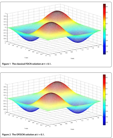
Figure 1 The classical FDCN solution att= 0.1.

Figure 2 The OFDCNI solution att= 0.1.

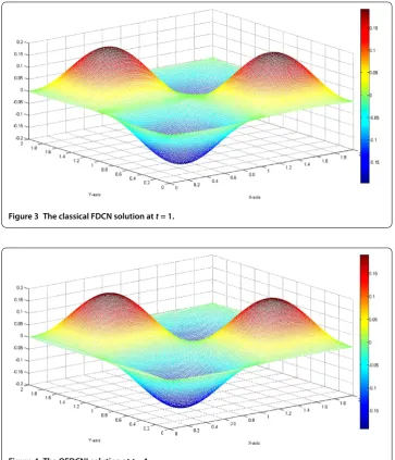
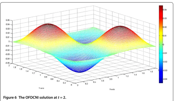
Comparing the numerical conclusions of the classical FDCN scheme with the OFDCNI scheme summarized the following conclusions. The charts in Figures  and  are basically identical at t= .. However, the classical FDCN solution appeared with a little disper-sion (see Figure ) att= ; whereas the OFDCNI solution was still stable and smooth (see Figure ). Especially, the classical FDCN solution emerged with very great dispersion (see Figure ) att=  due to the truncated error amassing, but the OFDCNI solution yet remained stable and smooth (see Figure ). It implies that the OFDCNI solutions were much better than the classical FDCN solutions and shows that the OFDCNI scheme is much more efficient and advanced than the classical FDCN scheme for solving the D Sobolev equation.

Figure 3 The classical FDCN solution att= 1.

Figure 4 The OFDCNI solution att= 1.

seconds in the same PC, but the errors of both solutions did not exceedO(–_{), which} also shows that the numerical computational results were in line with the theoretical ones. In addition, in the above numerical simulations, we only used the initial few given clas-sical FDCN solutions over a very short time span [,T] (TT) as the snapshots to constitute the POD basis and build the OFDCNI scheme before calculating the OFD-CNI solutions over the total time span [,T]. When one solves the real-world engineering problems, one may use the recorded data (over a very short time span [,T]) to constitute the POD basis, to build the OFDCNI scheme, and to predict future physical phenomena and changes (over a time span [T,T]). Therefore, the OFDCNI scheme holds very exten-sive applied prospect.

6 Conclusions

so-Figure 5 The classical FDCN solution att= 2.

Figure 6 The OFDCNI solution att= 2.

lutions for the D Sobolev equation. And then, the POD basis is constituted by the snap-shots, and the OFDCNI scheme having the fully second-order accuracy and containing very few unknowns is established by replacing the unknown FDCN solution vectors with the linear-combination of the POD basis. Finally, the stability and convergence of the OFD-CNI solutions are deduced. The numerical simulations have exhibited that the OFDOFD-CNI solutions are far better than the classical ones. This implies that the OFDCNI scheme is highly efficient and reliable for solving the D Sobolev equation.

Acknowledgements

This research was supported by the National Science Foundation of China grant (1167116) and the Fundamental Research Funds for the Central Universities (2016MS33).

Competing interests

The authors declare that they have no competing interests.

Authors’ contributions

All authors contributed equally and significantly in writing this article. All authors read and approved the final manuscript.

Author details

1_{School of Control and Computer Engineering, North China Electric Power University, No. 2, Bei Nong Road, Changping}

District, Beijing, 102206, China. 2_{School of Mathematics and Physics, North China Electric Power University, No. 2, Bei} Nong Road, Changping District, Beijing, 102206, China.

Publisher’s Note

Springer Nature remains neutral with regard to jurisdictional claims in published maps and institutional affiliations.

Received: 13 April 2017 Accepted: 22 June 2017

References

1. Davis, PL: A quasilinear parabolic and a related third order problem. J. Math. Anal. Appl.49, 327-335 (1970) 2. Ewing, RE: A coupled nonlinear hyperbolic system. Ann. Mat. Pura Appl.114(4), 331-349 (1977)

3. Barenblett, GI, Zheltov, IP, Kochian, IN: Basic concepts in the theory of seepage homogeneous liquids in fissured rocks. J. Appl. Math. Mech.24(5), 1286-1303 (1960)

4. Ting, TW: A cooling process according to two-temperature theory of heat conduction. J. Math. Anal. Appl.45(1), 23-31 (1974)

5. Shi, DM: On the initial boundary value problem of nonlinear equation of the migration of the moisture in soil. Acta Math. Appl. Sin.13(1), 31-38 (1990)

6. Cao, YH: The generalized difference scheme for linear Sobolev equation in two dimensions. Math. Numer. Sin.27(3), 243-256 (2005)

7. Ewing, RE: Time-stepping Galerkin methods for nonlinear Sobolev partial differential equations. SIAM J. Numer. Anal.

15(6), 1125-1150 (1978)

8. Li, H, Zhou, WW, Fang, ZC: Crank-Nicolson fully discrete finite element formulation for the Sobolev equations. Math. Numer. Sin.35(1), 40-48 (2013)

9. Li, H, Luo, ZD, An, J, Sun, P: A fully discrete finite volume element formulation for Sobolev equation and numerical simulation. Math. Numer. Sin.34(2), 163-172 (2012)

10. Ewing, RE: Numerical solution of Sobolev partial differential equations. SIAM J. Numer. Anal.12(3), 345-363 (1975) 11. Sun, TJ, Yang, DP: The finite difference streamline diffusion methods for Sobolev equations with

convection-dominated term. Appl. Math. Comput.125(2), 325-345 (2002)

12. Zhao, ZH, Li, H, Luo, ZD: A new space-time continuous Galerkin method with mesh modification for Sobolev equations. J. Math. Anal. Appl.440, 86-105 (2016)

13. Luo, ZD: A POD-based reduced-order TSCFE extrapolation iterative format for two-dimensional heat equations. Bound. Value Probl.2015, 59 (2015)

14. Liu, Y, Li, H, He, S, Gao, W, Mu, S: A new mixed scheme based on variation of constants for Sobolev equation with nonlinear convection term. Appl. Math. J. Chin. Univ. Ser. B28(2), 158-172 (2013)

15. Cazemier, W, Verstappen, RWCP, Veldman, AEP: Proper orthogonal decomposition and low-dimensional models for driven cavity flows. Phys. Fluids10, 1685-1699 (1998)

16. Dimitriu, G, Stefanescu, R, Navon, IM: POD-DEIM approach on dimension reduction of a multi-species host-parasitoid system. Ann. Acad. Rom. Sci. Ser. Math. Appl.7(1), 173-188 (2015)

17. Ghosh, R, Joshi, Y: Error estimation in POD-based dynamic reduced-order thermal modeling of data centers. Int. J. Heat Mass Transf.57, 698-707 (2013)

18. Holmes, P, Lumley, JL, Berkooz, G: Turbulence, Coherent Structures, Dynamical Systems and Symmetry. Cambridge University Press, Cambridge (1996)

19. Kunisch, K, Volkwein, S: Galerkin proper orthogonal decomposition methods for a general equation in fluid dynamics. SIAM J. Numer. Anal.40, 492-515 (2002)

20. Luo, ZD, Du, J, Xie, ZH, Guo, Y: A reduced stabilized mixed finite element formulation based on proper orthogonal decomposition for the non-stationary Navier-Stokes equations. Int. J. Numer. Methods Eng.88, 31-46 (2011) 21. Luo, ZD, Li, H, Zhou, YJ, Xie, ZH: A reduced finite element formulation and error estimates based on POD method for

two-dimensional solute transport problems. J. Math. Anal. Appl.385, 371-383 (2012)

22. Luo, ZD, Xie, ZH, Shang, YQ, Chen, J: A reduced finite volume element formulation and numerical simulations based on POD for parabolic problems. J. Comput. Appl. Math.235, 2098-2111 (2011)

23. Luo, ZD, Yang, XZ, Zhou, YJ: A reduced finite difference scheme based on singular value decomposition and proper orthogonal decomposition for Burgers equation. J. Comput. Appl. Math.229, 97-107 (2009)

24. Luo, ZD, Zhu, J, Wang, RW, Navon, IM: Proper orthogonal decomposition approach and error estimation of mixed finite element methods for the tropical Pacific Ocean reduced gravity model. Comput. Methods Appl. Mech. Eng.

196, 4184-4195 (2007)

25. Ly, HV, Tran, HT: Proper orthogonal decomposition for flow calculations and optimal control in a horizontal CVD reactor. Q. Appl. Math.60, 631-656 (2002)

27. Stefanescu, R, Sandu, A, Navon, IM: Comparison of POD reduced order strategies for the nonlinear 2D shallow water equations. Int. J. Numer. Methods Fluids76(8), 497-521 (2014)

28. Sun, P, Luo, ZD, Zhou, YJ: Some reduced finite difference schemes based on a proper orthogonal decomposition technique for parabolic equations. Appl. Numer. Math.60, 154-164 (2010)

29. Luo, ZD: A POD-based reduced-order finite difference extrapolating model for the non-stationary incompressible Boussinesq equations. Adv. Differ. Equ.2014, 272 (2014)

30. Luo, ZD, Gao, JQ: A POD-based reduced-order finite difference time-domain extrapolating scheme for the 2D Maxwell equations in a Lossy medium. J. Math. Anal. Appl.444, 433-451 (2016)

31. Luo, ZD, Jin, SJ, Chen, J: A reduced-order extrapolation central difference scheme based on POD for two dimensional fourth-order hyperbolic equations. Appl. Math. Comput.289, 396-408 (2016)

32. An, J, Luo, ZD, Li, H, Sun, P: Reduced-order extrapolation spectral-finite difference scheme based on POD method and error estimation for three-dimensional parabolic equation. Front. Math. China10(5), 1025-1040 (2015) 33. Zhang, WS: Finite Difference Methods for Partial Differential Equations in Science Computation. Higher Education

Press, Beijing (2006)