R E S E A R C H
Open Access
A fourth-order accurate quasi-variable
mesh compact finite-difference scheme for
two-space dimensional convection-diffusion
problems
Navnit Jha
*and Neelesh Kumar
*Correspondence: [email protected] Faculty of Mathematics and Computer Science, South Asian University, Akbar Bhawan, Chanakyapuri, New Delhi 110 021, India
Abstract
We discuss a new nine-point fourth-order and five-point second-order accurate finite-difference scheme for the numerical solution of two-space dimensional convection-diffusion problems. The compact operators are defined on a
quasi-variable mesh network with the same order and accuracy as obtained by the central difference and averaging operators on uniform meshes. Subsequently, a high-order difference scheme is developed to get the numerical accuracy of order four on quasi-variable meshes as well as on uniform meshes. The error analysis of the fourth-order compact scheme is described in detail by means of matrix analysis. Some examples related with convection-diffusion equations are provided to present performance and robustness of the proposed scheme.
MSC: 65N06; 65N12; 35J57; 35J72
Keywords: convection-diffusion equation; compact scheme; finite-difference method; quasi-variable meshes; irreducible and monotone matrix; maximum absolute error; root-mean squared error
1 Introduction
The two-dimensional elliptic equations
–ε∇U+a(x,y)Ux+b(x,y)Uy+c(x,y)U+d(x,y) = , (x,y)∈, (.) will be considered to develop numerical algorithms for computing the concentration U(x,y) of mass transfer. Here,εis viscosity coefficient or diffusion coefficient ( <ε) and (a(x,y),b(x,y)) > (β,β) > (, ) on(closure of= (, )×(, )) is velocity vector,
β,βare finite constants. We also assume thata(x,y),b(x,y),c(x,y),d(x,y) are continuous
andc(x,y)≥ onin order to ensure the existence of a solution. Let the following smooth boundary data be given:
U(,y) =ϕ(y), U(,y) =ϕ(y), ≤y≤, (.)
U(x, ) =ψ(x), U(x, ) =ψ(x), ≤x≤. (.)
The second-order partial derivatives in the mathematical model (.) describe the dif-fusion process, while the first-order partial derivatives are associated with the convection phenomenon. Whenε→, convection dominates the diffusion process, and the solution values of (.)-(.) exhibit boundary layer behavior, that is, solution changes rapidly in a small region, while outside the small region solution behavior is smooth. In two dimen-sions, the boundary layer may occur atx= andx= , known as normal layer, and/or at y= andy= , known as parallel layer, while the one-dimensional convection-diffusion problems exhibit only normal boundary layer []. Such type of a differential equation is said to be singularly perturbed. The solution of singular perturbation problems approaches a discontinuous limit as a small positive quantity (ε), known as perturbation parameter, ap-proaches zero. Thus, the analysis and numerical solution of singular perturbation prob-lems are significant.
The convection-diffusion problems occur in the area of fluid dynamics and several branches of applied mathematics. In the convection-diffusion process, transport phenom-ena prevail diffusion, whose effects are restricted to a small part of the domain and so-lution values exhibit multiple characters for small values of diffusion parameter. Thus, a second-order discretization of the Laplace operator may not ensure the consistency and stability of the numerical scheme []. The numerical schemes developed by the applica-tion of an upwind scheme and a central difference operator result in an unstable solu-tion and are deficient in computasolu-tional order. Any attempt to obtain solusolu-tion values up to the desired accuracies may land up in massive computing time despite a well-structured block-tridiagonal matrix of the difference equations received by the application of an up-wind scheme and central differences. Thus, acquiring improved finite-difference methods for convection-diffusion problems has a significant impact on numerical approximations of ordinary and partial differential equations [–]. The compact scheme amongst the various finite-difference replacements of convection-diffusion problems (.)-(.) has re-ceived more attention due to a minimal width of stencils in thex- andy-coordinate direc-tions and easy computadirec-tions. In contrast, high-order difference schemes formulated with non-compact stencils yield a higher bandwidth of the iteration matrix, and this involves large arithmetic operations. Numerical simulations with high-order compact difference schemes depict more accurate solution values on quasi-variable meshes as compared to some high-order compact scheme on a uniform mesh network. This happens because a truncation error in a finite-difference approximation depends upon the derivative of the variable as well as mesh spacing. Therefore, to attain uniformly distributed truncation errors, it is essential to employ non-uniform meshes, i.e., finer meshes in the region for largely deviated derivatives and coarse meshes for a smooth function. In this manner, the error disperses almost uniformly over the domain of integration and renders an accurate solution to a greater extent. Thus, high-order finite-difference discretization formulated on a quasi-variable mesh network leads to more precise numerical solutions and brings unconditional numerical stability [].
meshes for the Helmholtz equation and solved the difference equations with the help of the multigrid method. Jha [, ] developed a third-order exponential expanding mesh compact scheme for mildly non-linear elliptic equations. The Galerkin and Petrov-Galerkin finite element method for determining the approximate solution values to the two-dimensional convection-diffusion problems were discussed by Hegarty []. A nine-point tailored finite nine-point method for solving convection-diffusion-reaction equation was developed by Shih et al. []. In the context of one dimension, the finite-difference re-placement of a convection-diffusion equation was extensively discussed in [, ], and non-uniform mesh compact finite-difference operators for first- and second-order ordi-nary derivatives associated with the Numerov fourth-order method were obtained in [, ]. Finite-difference methods for convection-diffusion problems showing exponential or parabolic boundary layer behavior were described in detail by Roos et al. [].
The work presented in this article is organized in the following manner. In Section , we describe two-dimensional quasi-variable meshes to deal with parallel and normal layer by means of mesh parameters in thex- andy-directions. Section discusses compact oper-ators and high-order approximations of first- and second-order derivatives on minimum stencils. A new compact scheme of fourth-order accuracy using quasi-variable meshes has been obtained. The suggested scheme is analyzed for the convergence and the bounds of the discretization error are obtained in Section . Numerical simulations with some convection-diffusion problems that exhibit normal and/or parallel layers are carried out in Section . The paper is concluded at last with remarks and further scope.
2 Quasi-variable meshes
LetLandMbe positive integers, and divide the domain [, ]×[, ] into (L+ )(M+ ) cells with the coordinates (xl,ym), wherex= ,xl=xl–+hl,l= ()L,xL+= andy= ,
ym=ym–+km,m= ()M, yM+= . The mesh step-size is determined by the
stretch-ing functions hl+ =hl( +αhl), l= ()L and km+ =km( +βkm), m= ()M, by suit-ably chosen normalization α˜ =αh andβ˜=βk. Since the length of a diffusion space
along thex-direction is one, for a given value ofα˜, the relationLl=+hl= easily pro-duces the first mesh step-size h in the x-direction (and similarly in the y-direction).
As an example, h = /( + α˜) ifL= . In particular, if α=β = , the meshes are
uni-formly distributed andh=hl,k=km,∀l,m. The mesh step-size is increasing if and only if hl<hl+∀l= ()L⇔hl<hl( +αhl)⇔α> . In a similar manner, we can prove that the mesh step-size is decreasing whenα< . Therefore, the mesh-step sequences{hl}Ll=+and, similarly,{km}Mm=+are monotonic.
Let us consider the uniform mesh partition of the domainP=[, ] ={pl=lh,l= ()L+ }, h= /(L+ ). Since the mesh-step sequence is monotonic, it is possible to define a one-one onto mapψ:P−→P such thatψ(pl) =xl,l= ()L+ , and the JacobianJ(p) = dψ(p)/dpis bounded above and below by some positive constants as <n≤J(p)≤N<
∞,∀p∈P. Therefore,
J(p) > ⇒ dψ(p)
dp > ⇒
ψ(pl+) –ψ(pl)
pl+–pl
> ⇒ xl+–xl (l+ )h–lh>
Also,J(p)≤N⇒dψdp(p)≤N⇒ ψ(pl+)–ψ(pl)
Thus, the maximum step-size along thex-direction diminishes with the growth of mesh points. Likewise, the maximum step-size along they-direction approaches to zero ifM is very large. Thus, we observed that the mesh step-size is inversely proportional to the number of mesh points.
Sundqvist and Veronis [] initially discussed such a mesh network in the context of wind-driven ocean circulation, and later the application to digital electrochemistry was described by Britz []. Some compact operators related to a quasi-variable mesh were mentioned in the literature [, ].
3 Finite-difference schemes and compact operators
The operators used to obtain first- and second-order partial derivatives with a mini-mum stencil width are known as compact. The high-order finite-difference replacement of equation (.) requires discretization of partial derivatives, and thus we consider the following approximations:
Now, we define the following operators:
PxUl,m=hlU
hl,k=km,∀l,m, thenPx= μxδxandQx=δx, whereμxandδxare averaging and central differencing operators in thex-direction [].
By means of operators (.)-(.) it is easy to approximate partial- and mixed-order derivatives of an analytic functionG(x,y) at the mesh point (xl,ym) in the following man-ner:
Gxl,m=h–l PxGl,m+ O
hl, Gyl,m=km–PyGl,m+ O
km, (.)
Gxxl,m=h–l QxGl,m+ O
hl, Gyyl,m=k–mQyGl,m+ O
km, (.)
Gxyl,m=h–l km–PxPyGl,m+ O
hl +km. (.)
An immediate application of these operators to equation (.) yields a five-point second-order accurate discretization scheme. Such kind of a second-second-order method on a variable mesh network is known assupra-convergent scheme [].
Now, we describe a new fourth-order scheme for linear Poisson’s equation and then extend it to the elliptic equation (.), which involves convection termsUx=∂U/∂xand Uy=∂U/∂y.
By means of a linear combination of functional valuesGρ,σ =G(xρ,yσ), (ρ,σ)∈D=
{l– ,l,l+ } × {m– ,m,m+ }, the finite-difference replacement for a simple form of two-space dimensional elliptic equations (Poisson’s equation)
–ε∇U+G(x,y) = (.)
is given by
–∇hl,kmUl,m+hlkmLGl,m=Tl,m, l= ()L,m= ()M, (.)
where
∇
hl,km≡ε
kmQx+hlQy+ε
αhlPxQy+βkmPyQx
+ ε
hl( +αhl) +km( +βkm)QxQy (.)
is a discrete form of the Laplace operator∇=∂
x+∂y,
L≡ +hl αPx+
km βPy+
hlkm
αβPxPy+
( +αhl)Qx+
( +βkm)Qy, (.)
andTl,mis the local truncation error calculated as
Tl,m=hlkmO
hl +hlkm+km. (.)
The eighth-order of local truncation error obtained here is irrespective of mesh param-etersα,βbeing chosen zero or non-zero. Since the operatorLin equation (.) is multi-plied byh
Our main aim is to extend the fourth-order method (.) to the convection-dominated equation (.) that comprises first-order partial derivatives in thex- andy-directions along with the functionU(x,y).
Let us consider
Fρ,σ=aρ,σU x
ρ,σ +bρ,σU y
ρ,σ +cρ,σUρ,σ+dρ,σ, (ρ,σ)∈ ˆD=D∼
(l,m), (.)
Uxl,m=Uxl,m+hlαFl+,m+αFl–,m+αU
yy
l+,m+αU
yy l–,m
, (.)
Uyl,m=Uyl,m+kmβFl,m++βFl,m–+βU
xx
l,m++βU
xx l,m–
, (.)
Fl,m=al,mU
x
l,m+bl,mU
y
l,m+cl,mUl,m+dl,m, (.)
whereαi,βi,i= () are unknown parameters to be measured in such a way that
L(Fl,m–Gl,m) =O
hl+hlkm +km. (.)
By making use of (.), (.)-(.) and (.), the algebraic calculations give us
α= –( +αhl)/
ε( +αhl)
, α= –α– αhl/
ε +αhl+βkm,
β= –( +βkm)/
ε( +βkm)
, β= –β– βkm/
ε +αhl+βkm,
α= –εα, α= –εα, β= –εβ, β= –εβ.
As a result, we obtain a single compact discretization scheme
–∇hl,kmUl,m+hlkmLFl,m=Tl,m, l= ()L,m= ()M, (.) that numerically approximates equation (.) with fourth-order accuracy on a quasi-variable mesh network as well as on a uniform mesh network. The discretization (.) yields a non-symmetric matrix after incorporating the boundary values (.)-(.) as
U,m=ϕ(ym), UL+,m=ϕ(ym), m= ()M+ , (.)
Ul,=ψ(xl), Ul,M+=ψ(xl), l= ()L+ . (.)
The lexicographical ordering of the unknown valuesUl,min equation (.) gives rise to a block tri-diagonal linear system of equations and can be easily computed by means of the Gauss-Seidel iterative formula. For the programming, we must neglect the truncation errorTl,mfrom equation (.) and replace the exact valueUl,m=U(xl,ym) by its approx-imate valueul,m.
4 Convergence analysis and error bounds
In this section, we discuss the upper bounds of discretization errors and derive the nec-essary convergence conditions for scheme (.). The compact scheme (.) determines the exact solution valuesU= [Ul,m], and in terms of the mesh-ratio parameterζl,m=km/hl, it can be expressed as
whereTl,m=O(hl) and
∇
hl,km=h –
l ∇hl,km≡ε
ζl,mQx+Qy+ε hl
αPxQy+βζl,mPyQx
+ ε
+αhl+ζl,m( +βhlζl,m)
QxQy.
Our aim is to compute approximate solution vectoru= [ul,m] that satisfies
–∇hl,kmul,m+hlζl,mLfl,m= , l= ()L,m= ()M, (.) where
fp,q=aρ,σuxρ,σ +bρ,σuyρ,σ+cρ,σuρ,σ +dρ,σ≈Fρ,σ, (ρ,σ)∈ ˆD, (.) fl,m=al,mu
x
l,m+bl,mu y
l,m+cl,mul,m+dl,m≈Fl,m (.) and the formula foruxρ,σ,uyρ,σ, (ρ,σ)∈ ˆDis obtained from (.), andu
x l,m,u
y
l,mare obtained from (.)-(.) upon replacing the symbolUbyu.
Let=U–ube the discretization error vector andl,m=Ul,m–ul,m,l= ()L,m= ()M be the point-wise error.
By subtracting (.) from (.), the discretization error satisfies the relation
–∇hl,kml,m+hlζl,mLEl,m=Tl,m, l= ()L,m= ()M, (.) whereEρ,σ =Fρ,σ–fρ,σ, (ρ,σ)∈Dand to be explicit
Eρ,σ =aρ,σρx,σ+bρ,σyρ,σ +cρ,σρ,σ, (ρ,σ)∈ ˆD, (.) El,m=al,m
x
l,m+bl,m y
l,m+cl,ml,m. (.)
Here, the expressions forxρ,σ,yρ,σ, (ρ,σ)∈ ˆDandxl,m,yl,mare obtained from equations (.) and (.)-(.), respectively, upon interchange ofUby.
Representing the system of linear equations (.) in a matrix-vector form, one obtains
M+T=0, (.)
whereT(hl) = [Tl,m]tl=()L,m=()Mis the sixth-order error vector andM= [Mi,j]i,j=()LM= [R S R] is the block tri-diagonal coefficient matrix and, in particular, whenmaxlhl→, that is, for a sufficiently small value of mesh spacing, we find
R= ε
–( +ζi,j) –( –ζi,j) –( +ζi,j)
and
S=ε
–(ζi,j– ) ( +ζi,j) –(ζi,j– )
as tri-diagonal matrices.
Theorem . The block tri-diagonal matrixM is irreducible provided the mesh-ratio parameterζi,j∈(/
√
Proof It is evident that the matrixM has positive diagonal values sinceζi,j is positive for alliandj. Further,Mhas non-positive off-diagonal values provided /√ <ζi,j<
√
. Now, if we labelLMdistinct points in thexy-plane as , , . . . ,LMand draw an arrow from itojsuch thatMi,j= , then, for any two distinct pointsiandj, there exists a directed path that joins the ordered pair of nodesiandj. Therefore, the graphG(M) of the matrixM is connected, and henceMis an irreducible matrix [, ]. This completes the proof.
Theorem . For a sufficiently small value of mesh step-sizes and c(x,y)≥,the block tri-diagonal matrixMis monotone.
Proof Letζ=minl,mζl,m,c=minl,mcl,m,l= ()L,m= ()M, andϑj, (j= , . . . ,LM) denote thejthrow element sum of the matrixM. Sincec(x,y)≥, thereforec=minl,mc(xl,ym)≥ . Thus, for a sufficiently small mesh step-size (i.e.,maxlhl→), the following asymptotic bounds on the weak row sums can be computed:
ϑj≥ ε
+ζ> , j= ,L,
ϑj≥ε> , j= ()L– ,
ϑ(r–)L+j≥εζ> , r= ()M– ,j= ,L,
ϑ(r–)L+j≥
⎧ ⎨ ⎩
cζh
, α> ,
cζh
L+, α< ,
r= ()M– ,j= ()L– ,c≥
ϑ(M–)L+j≥ ε
+ζ> , j= ,L,
ϑ(M–)L+j≥ε> , j= ()L– .
Note that, except corresponding to the main diagonal, all of the weak row element sums are positive and off-diagonal values of the matrixMare non-positive for sufficiently small values of mesh step-size. SinceMis irreducible (Theorem .), it follows that the matrix
Mis monotone, and this completes the proof.
Theorem . The matrixMis monotone if and only if the elements of the inverse matrix
M–are non-negative.
Proof See Henrici [].
Theorem . If h=maxlhl,then∞≤O(h).
Proof By means of Theorems . and ., one obtains that the matrixMis invertible and
M–≥. For notational convenience, we denoteM–= [M–
i,j]i,j=()LM,andIis a matrix of orderLM× having all entries as one. Then the matrix identityM–(MI) =Igives rise to
LM
j=
M–
Ifh=maxlhl, thenh=hforα< andh=hL+forα> . Thus, in view of eachM–i,j ≥
The matrix-vector norm in the following analysis is taken to be
M–
As a result of combining the above inequalities and equation (.), we obtain
∞≤M–∞·T∞≤ Theorem . corroborates the fourth-order convergence of the new compact scheme (.) for obtaining the numerical solution values of convection-dominated problems (.)-(.) in the quasi-variable mesh network. Note that the restrictionc=minl,mcl,m≥ in (.) pertains the assumptionc(x,y)≥ onin Section .
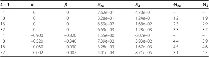
5 Comparison of numerical and exact solution values
Table 1 Accuracies in solution values atε= 10–2in Example 5.1
4 –0.900 –0.820 1.55e–00 6.07e–01 – –
8 –0.520 –0.340 7.39e–02 3.93e–02 4.4 3.9
16 –0.060 –0.090 3.28e–03 1.67e–03 4.5 4.6
32 –0.002 –0.007 4.01e–04 8.71e–05 3.1 4.3
convergence order are computed by means of the formulas
E=
The above estimates are obtained using quasi-variable meshes (α= orβ= ) as well as for constant mesh step-size (α= andβ= ). To ease the computational work, we have takenL=M, and Dirichlet’s boundary values are received from the known analytic solutions. The Gauss-Seidel iterative method for the solution of linear difference equations uses the tolerance of error as –[]. Simulations with second-order accuratesupra
-convergent scheme show slow converging results, and thus they are not mentioned in the tabulated results. The Maple’sCodeGenerationtool symbolically obtained the compact schemes, and C programming on the Macintosh operating system performed numerical computing.
Example .([, ]) Consider the singularly perturbed problems
ε∇U(x,y) =
behavior of the solution changes sharply and can be easily captured by means of the quasi-variable mesh compact scheme as presented in Table .
Example .([]) Consider the constant coefficients convection-diffusion problem
∇U(x,y) =ηUx(x,y) +ηUy(x,y) –δU(x,y) +g(x,y), <x,y< .
Table 2 Accuracies in solution values in Example 5.2 withη= 100π,δ= 30π2
L + 1 α˜ β˜ E∞ E2 ∞ 2
4 0 0 5.82e–02 3.52e–02 – –
8 0 0 2.39e–02 1.16e–02 1.3 1.6
16 0 0 6.07e–03 2.38e–03 2.0 2.3
32 0 0 6.00e–04 2.02e–04 3.3 3.6
4 0.440 0.2900 7.39e–02 4.01e–02 – –
8 0.280 0.2700 8.58e–03 1.59e–03 3.1 4.7
16 0.103 0.1020 2.61e–04 8.93e–05 4.9 4.2
32 0.000 0.0423 4.35e–05 5.15e–06 2.6 4.1
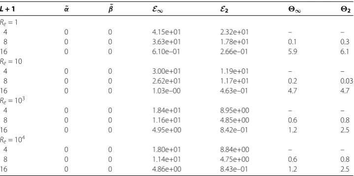
Table 3 Accuracies in solution values with uniform meshes in Example 5.3
L + 1 α˜ β˜ E∞ E2 ∞ 2
Re= 1
4 0 0 4.15e+01 2.32e+01 – –
8 0 0 3.63e+01 1.78e+01 0.1 0.3
16 0 0 6.10e–01 2.66e–01 5.9 6.1
Re= 10
4 0 0 3.00e+01 1.19e+01 – –
8 0 0 2.62e+01 1.17e+01 0.2 0.03
16 0 0 1.03e–00 4.63e–01 4.7 4.7
Re= 103
4 0 0 1.84e+01 8.95e+00 – –
8 0 0 1.16e+01 4.85e+00 0.6 0.8
16 0 0 4.95e+00 8.42e–01 1.2 2.5
Re= 104
4 0 0 1.80e+01 8.84e+00 – –
8 0 0 1.14e+01 4.75e+00 0.6 0.8
16 0 0 4.86e+00 8.43e–01 1.2 2.5
coarse quasi-variable meshes, whereas the uniform mesh solution values deteriorate in both order and accuracies as shown in Table .
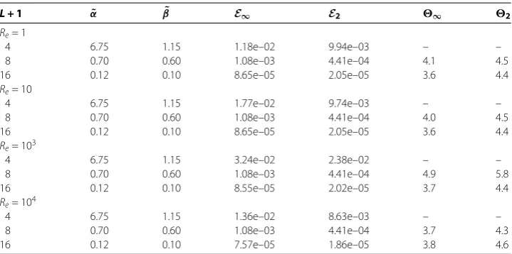
Example .([]) Consider the variable coefficient two-space dimensional convection-diffusion equation on a rectangular domain <x,y< :
ε∇U(x,y) =x– (y– )Ux(x,y) + xy( –y)Uy(x,y) +g(x,y).
The analytical solution is U(x,y) =sin(πx) +sin(πx) +cos(πx) +cos(πx). Here, ε= /Re andRe is the Reynolds number. Table presents the error in solution values from lower to higher Reynolds number (≤Re≤) by using the uniform mesh compact scheme, and the expected computational order of accuracy is not achieved. At the same time, the fourth-order compact method on quasi-variable meshes yields a satisfactory re-sult as shown in Table .
6 Concluding remarks
Table 4 Accuracies in solution values with quasi-variable meshes in Example 5.3
L + 1 α˜ β˜ E∞ E2 ∞ 2
Re= 1
4 6.75 1.15 1.18e–02 9.94e–03 – –
8 0.70 0.60 1.08e–03 4.41e–04 4.1 4.5
16 0.12 0.10 8.65e–05 2.05e–05 3.6 4.4
Re= 10
4 6.75 1.15 1.77e–02 9.74e–03 – –
8 0.70 0.60 1.08e–03 4.41e–04 4.0 4.5
16 0.12 0.10 8.65e–05 2.05e–05 3.6 4.4
Re= 103
4 6.75 1.15 3.24e–02 2.38e–02 – –
8 0.70 0.60 1.08e–03 4.41e–04 4.9 5.8
16 0.12 0.10 8.55e–05 2.02e–05 3.7 4.4
Re= 104
4 6.75 1.15 1.36e–02 8.63e–03 – –
8 0.70 0.60 1.08e–03 4.41e–04 3.7 4.3
16 0.12 0.10 7.57e–05 1.86e–05 3.8 4.6
coarse quasi-variable meshes make the algorithm more efficient in comparison with uni-formly spaced fine meshes despite the fact that both of them are fourth-order accurate methods. The new method improves maximum absolute and root mean squared errors of solution values as well as their computational order of convergence. It is possible to extend such a technique to three-dimensional convection-diffusion problems.
Competing interests
The authors declare that they have no competing interest.
Authors’ contributions
NJ discussed the quasi-variable meshes andsupra-convergent scheme. NK described the high-order compact scheme and matrix analysis of the difference equations. NJ and NK jointly obtained numerical results. All authors read and approved the final manuscript.
Received: 21 November 2016 Accepted: 13 February 2017
References
1. Segal, A: Aspects of numerical methods for elliptic singular perturbation problems. SIAM J. Sci. Comput.3, 327-349 (1982)
2. Stynes, M: Steady-state convection-diffusion problems. Acta Numer.14, 445-508 (2005)
3. Tian, ZF, Dai, SQ: High-order compact exponential finite difference methods for convection-diffusion type problems. J. Comput. Phys.220, 952-974 (2007)
4. Thomas, JW: Numerical Partial Differential Equations: Conservation Laws and Elliptic Equations. Springer, New York (1999)
5. Boisvert, RF: Families of high order accurate discretization of some elliptic problems. SIAM J. Sci. Stat. Comput.2, 268-285 (1981)
6. Strikwerda, JC: Finite Difference Schemes and Partial Differential Equations. SIAM, Philadelphia (2004) 7. Ferziger, JH, Peric, M: Computational Methods for Fluid Dynamics. Springer, Berlin (2002)
8. Mishra, N, Sanyasiraju, VSSY: Efficient exponential compact higher order difference scheme for convection dominated problems. Math. Comput. Simul.82, 617-628 (2011)
9. Mohanty, RK, Setia, N: A new compact high order off-step discretization for the system of 2D quasi-linear elliptic partial differential equations. Adv. Differ. Equ.2013, 223 (2013)
10. Saldanha, G, Ananthakrishnaiah, U: A fourth-order finite difference scheme for two-dimensional nonlinear elliptic partial differential equations. Numer. Methods Partial Differ. Equ.11, 33-40 (1995)
11. Zhai, S, Feng, X, He, Y: A new method to deduce high-order compact difference schemes for two-dimensional Poisson equation. Appl. Math. Comput.230, 9-26 (2014)
12. Mohanty, RK, Singh, S: A new fourth order discretization for singularly perturbed two dimensional non-linear elliptic boundary value problems. Appl. Comput. Math.175, 1400-1414 (2006)
13. Zhang, J, Kouatchou, J, Ge, L: A family of fourth-order difference schemes on rotated grid for two-dimensional convection-diffusion equation. Math. Comput. Simul.59, 413-429 (2002)
14. Ghaffar, F, Badshah, N, Islam, S, Khan, MA: Multigrid method based on transformation-free high-order scheme for solving 2D Helmholtz equation on nonuniform grids. Adv. Differ. Equ.201619 (2016)
16. Jha, N, Kumar, N, Sharma, KK: A third (four) order accurate, nine-point compact scheme for mildly-nonlinear elliptic equations in two space variables. Differ. Equ. Dyn. Syst. (2015). doi:10.1007/s12591-015-0263-9
17. Hegarty, AF, O’Riordan, E, Stynes, M: A comparison of uniformly convergent difference schemes for two-dimensional convection-diffusion problems. J. Comput. Phys.105, 24-32 (1993)
18. Shih, Y, Kellogg, RB, Tsai, P: A tailored finite point method for convection-diffusion- reaction problems. J. Sci. Comput.
43, 239-260 (2010)
19. Kadalbajoo, MK, Sharma, KK: A numerical method based on finite difference for boundary value problems for singularly perturbed delay differential equations. Appl. Math. Comput.197, 692-707 (2008)
20. Natesan, S, Ramanujam, N: Booster method for singularly perturbed one-dimensional convection-diffusion Neumann problems. J. Optim. Theory Appl.99, 53-72 (1998)
21. Bieniasz, LK: A set of compact finite-difference approximations to first and second derivatives, related to the extended Numerov method of Chawla on non-uniform grids. Computing.81, 77-89 (2007)
22. Manteuffel, TA, White, AB: The numerical solution of second-order boundary value problems on nonuniform meshes. Math. Comput.47, 511-535 (1986)
23. Roos, HG, Stynes, M, Tobiska, L: Robust Numerical Methods for Singularly Perturbed Differential Equations: Convection-Diffusion-Reaction and Flow Problems, vol. 24. Springer, Berlin (2008)
24. Sundqvist, H, Veronis, G: A simple finite-difference grid with non-constant intervals. Tellus A22, 26-31 (1970) 25. Britz, D: Digital Simulation in Electrochemistry. Springer, Berlin (2005)
26. Samarskii, AA, Matus, PP, Vabishchevich, PN: Difference Schemes with Operator Factors. Springer, Berlin (2002) 27. Saul’yev, VK: Integration of Equations of Parabolic Type by the Method of Nets, vol. 54. Elsevier, Amsterdam (2014) 28. Jain, MK, Iyengar, SRK, Jain, RK: Computational Methods for Partial Differential Equations. Wiley, New York (1994) 29. Kreiss, HO, Manteuffel, TA: Supra-convergent schemes on irregular grids. Math. Comput.47(176), 537-554 (1986) 30. Young, DM: Iterative Solution of Large Linear Systems. Elsevier, Amsterdam (2014)
31. Varga, RS: Matrix Iterative Analysis. Springer, Berlin (2000)
32. Henrici, P: Discrete Variable Methods in Ordinary Differential Equations. Wiley, New York (1962) 33. Saad, Y: Iterative Methods for Sparse Linear Systems. SIAM, Philadelphia (2003)