R E S E A R C H
Open Access
Dynamics of a delayed SEIRS-V model on the
transmission of worms in a wireless sensor
network
Zizhen Zhang
*and Fengshan Si
*Correspondence:
School of Management Science and Engineering, Anhui University of Finance and Economics, Bengbu, 233030, P.R. China
Abstract
A delayed SEIRS-V model on the transmission of worms in a wireless sensor network is considered. Choosing delay as a bifurcation parameter, the existence of the Hopf bifurcation of the model is investigated. Furthermore, we use the normal form method and the center manifold theorem to determine the direction of the Hopf bifurcation and the stability of the bifurcated periodic solutions. Finally, some numerical simulations are presented to verify the theoretical results.
Keywords: Hopf bifurcation; delay; SEIRS-V model; stability; periodic solution; wireless sensor network
1 Introduction
In past several decades, many authors have studied different mathematical models which illustrate the dynamical behavior of the transmission of computer viruses based on the classical epidemic models due to the lots of similarities between biological viruses and computer viruses [–]. In [], Yuan and Chen investigated the behavior of virus propa-gation in a network by proposing an e-SEIR model. In [], Mishra and Pandey proposed an SEIRS model to investigate the transmission of worms in a network. As wireless sensor networks are unfolding their vast potential in a plethora of application environments, se-curity still remains one of the most critical challenges yet to be fully addressed [, ]. In order to study the attacking behavior of possible worms in a wireless sensor network and considering that there is a basic similarity between the software viruses spread among wireless devices and the transmission of epidemic diseases in a population, Mishra and Keshri [] proposed the following SEIRS-V model:
⎧ ⎪ ⎪ ⎪ ⎪ ⎪ ⎪ ⎪ ⎨ ⎪ ⎪ ⎪ ⎪ ⎪ ⎪ ⎪ ⎩
dS(t)
dt =A–βS(t)I(t) – (μ+p)S(t) +δR(t) +ηV(t), dE(t)
dt =βS(t)I(t) – (μ+α)E(t), dI(t)
dt =αE(t) – (μ+ε+γ)I(t), dR(t)
dt =γI(t) – (μ+δ)R(t), dV(t)
dt =pS(t) – (μ+η)V(t),
()
whereS(t),E(t),I(t),R(t) andV(t) represent the numbers of sensor nodes at timetin states susceptible, exposed, infectious, recovered and vaccinated, respectively.Ais the inclusion
of new nodes to the wireless sensor network,βis the transmission coefficient.α,γ,δ,η
andpare state transition rates.εandμare the crashing rates of the sensor nodes due to the attack of worms and the reason other than the attack of worms, respectively. Mishra and Keshri [] studied the stability of system ().
As is known, computer virus models with time delay have been investigated by many authors [–]. In [], Fenget al.investigated a viral infection model in computer net-works with time delay due to the temporary immunity period of the recovered computers. In [], Donget al.proposed a computer virus model with time delay due to the time that the computers in a network use antivirus software to clean the viruses and investigated the Hopf bifurcation of the model by choosing the delay as a bifurcation parameter. Moti-vated by the work above, and considering that the sensor nodes need some time to clean the worms in a wireless sensor network by using antivirus software and the recovered and the vaccinated sensor nodes have a temporary immunity period after which they may be infected again because of antivirus software, we incorporate two delays into system () and get the following delayed SEIRS-V system on the transmission of worms in a wireless sensor network:
where τ is the time that the sensor nodes need to clean the worms by using antivirus
software andτis the temporary immunity period after which they may be infected again
because of antivirus software. For the convenience of analysis, we assume thatτ=τ. Let
τ=τ, then system () becomes
This paper is organized as follows. In Section , we investigate local stability of the pos-itive equilibrium and obtain sufficient conditions for the existence of local Hopf bifurca-tion. In Section , we determine direction and stability of the Hopf bifurcation by using the normal form theory and the center manifold theorem. In order to testify the theoreti-cal analysis, a numeritheoreti-cal example is presented in Section . Section concludes the paper and indicates future directions for research.
R∗= γ
μ+δI∗, V=
p(μ+α)(μ+ε+γ)
αβ(μ+η) ,
I∗=αβA(μ+δ)(μ+η) +β(μpη(μ++α)(μα)(μ++δ)(μδ)(μ++η)(με+γ+) – (μ+p)(μ+α)(μ+δ)(μ+η)(μ+ε+γ)
ε+γ) –αβδγ(μ+η) .
The Jacobian matrix of system () about the positive equilibriumD∗is
J(D∗) =
⎛ ⎜ ⎜ ⎜ ⎜ ⎝
λ–a –a –be–λτ –be–λτ
–a λ–a –a
–a λ–a–be–λτ
–be–λτ λ–a–be–λτ
–a λ–a–be–λτ
⎞ ⎟ ⎟ ⎟ ⎟ ⎠,
where
a= –(βI∗+μ+p), a= –βS∗, a=βI∗,
a= –(μ+α), a=βS∗, a=α,
a= –(μ+ε), a= –μ, a=p, a= –μ,
b=δ, b=η, b= –γ,
b=γ, b= –δ, b= –η.
Thus, the characteristic equation of system () atD∗is
λ+Aλ+Aλ+Aλ+Aλ+A+Bλ+Bλ+Bλ+Bλ+Be–λτ
+Cλ+Cλ+Cλ+C
e–λτ+D
λ+Dλ+D
e–λτ= , ()
where
A= –aa(aaa+aaa),
A=aaa(a+a) +aaa(a+a)
+aaaa+aaa(a+a),
A= –aaa+aa+ (a+a)(a+a)
–aaa–aa(a+a) –aa(a+a),
A=aa+aa+ (a+a)(a+a)
+a(a+a+a+a),
A= –(a+a+a+a+a),
B=aab(aa–aa) –aaa(ab+ab)
–aa(aab+aab+aab),
B=baa(a+a) +aa(a+a)+aaa(b+b)
+baa(a+a) +aa(a+a)
+ab(aa–aa–aa–aa),
B=ab(a+a+a) –baa+aa+ (a+a)(a+a)
–baa+aa+ (a+a)(a+a)
–baa+aa+ (a+a)(a+a),
B=b(a+a+a+a) +b(a+a+a+a)
+b(a+a+a+a) –ab,
B= –(b+b+b), C=bb+bb+bb,
C=ab(b+b) –bb(a+a+a) –bb(a+a+a)
–bb(a+a+a),
C=bb
aa+a(a+a)
–aabb+bb
aa+a(a+a)
+bb
aa+a(a+a)
–ab
b(a+a) +b(a+a)
,
C=ab(aab+aab–aab) +aa(abb–abb)
–aa(abb+abb+abb),
D= –bbb, D=bbb(a+a) –abbb,
D=aabbb+aabbb–aaabb.
Multiplyingeλτon both sides of Eq. (), it is easy to obtain
Bλ+Bλ+Bλ+Bλ+B+λ+Aλ+Aλ+Aλ+Aλ+Aeλτ
+Cλ+Cλ+Cλ+Ce–λτ+Dλ+Dλ+De–λτ= . () Whenτ= , Eq. () reduces to
λ+mλ+mλ+mλ+mλ+m= , ()
where
m=A+B+C+D, m=A+B+C+D,
m=A+B+C+D, m=A+B+C,
m=A+B=p+α+δ+ε+γ+η+βI∗+ μ.
Obviously,m> . By the Routh-Hurwitz criterion, sufficient conditions for all roots of Eq. () to have a negative real part are given in the following form:
D=det
m
m m
> , ()
D=det
⎛ ⎜ ⎝
m
m m m
m m
⎞ ⎟
D=det
⎛ ⎜ ⎜ ⎜ ⎝
m
m m m
m m m m
m m
⎞ ⎟ ⎟ ⎟
⎠> , ()
D=det
⎛ ⎜ ⎜ ⎜ ⎜ ⎜ ⎜ ⎝
m
m m m
m m m m m
m m m
m
⎞ ⎟ ⎟ ⎟ ⎟ ⎟ ⎟ ⎠
> . ()
Thus, if condition (H) Eq. ()-Eq. () holds,D∗is locally asymptotically stable in the
absence of delay.
Forτ > , letλ=iω(ω> ) be the root of Eq. (). Then we can get
gcosτ ω–gsinτ ω+g=hsinτ ω+hcosτ ω,
gsinτ ω+gcosτ ω+g=hcosτ ω–hsinτ ω, where
g=Aω– (A+C)ω+A+C,
g=ω– (A–C)ω+ (A–C)ω,
g=Bω–Bω+B,
g=Aω– (A–C)ω+A–C, g=ω– (A+C)ω+ (A+C)ω,
g=Bω–Bω, h= –Dω, h=Dω–D.
Then we can get
(gcosτ ω–gsinτ ω+g)+ (gsinτ ω+gcosτ ω+g)=h+h. () According tosinτ ω=±√ –cosτ ω, we consider the following two cases.
Case .sinτ ω=√ –cosτ ω, then Eq. () becomes
gcosτ ω–g√ –cosτ ω+g+g√ –cosτ ω+gcosτ ω+g
=h+h, ()
which is equivalent to
ecosτ ω+ecosτ ω+ecosτ ω+ecosτ ω+e= , ()
where
e=g+g+g+g–h–h– (gg–gg),
– (gg–gg)(gg–gg), sinτ ω. Thus, a function with respect toωcan be established by
If all the parameters of system () are given, we can calculate the roots of Eq. () by Matlab software package. Therefore, we make the following assumption in order to give the main results in this paper.
(H) Eq. () has finite positive roots which are denoted byω,ω, . . . ,ωk, respectively. For every fixedωi(≤i≤k), the corresponding critical value of time delay is
τi(j)=
ωi
arccosf(ωi) + jπ
ωi
, i= , , . . . ,k,j= , , , . . . .
Case .sinτ ω= –√ –cosτ ω, then Eq. () becomes
gcosτ ω+g√ –cosτ ω+g+gcosτ ω–g√ –cosτ ω+g
=h+h. ()
Similar as in Case , we can get the expression ofcosτ ωdenoted asf∗(ω) and the
ex-pression ofsinτ ωdenoted byf∗(ω), and further we get a function with respect toωthat can be established by
f∗(ω) +f∗(ω) = . ()
We assume that Eq. () has finite positive roots denoted byω,ω, . . . ,ωk, respectively. Then we can get the critical value of time delay corresponding to every fixed positive root
ωiof Eq. ():
τi(j)=
ωiarccosf∗
ωi+jπ
ωi , i= , , . . . ,k,j= , , , . . . .
Let
τ=min
τi(),τi(), i= , , . . . ,k.
Then, whenτ =τ, Eq. () has a pair of purely imaginary roots±iω.
Next, we verify the transversality condition. Taking the derivative ofλwith respect toτ
in Eq. (), it is easy to obtain
dλ
dτ
–
=g(λ) +g(λ)e
λτ+g
(λ)e–λτ+g(λ)e–λτ h(λ) –h(λ)eλτ –
τ λ,
with
g(λ) = Bλ+ Bλ+ Bλ+B,
g(λ) = λ+ Aλ+ Aλ+ Aλ+A,
g(λ) = Cλ+ Cλ+C,
g(λ) = Dλ+D,
h(λ) =Cλ+ (C+ D)λ+ (C+ D)λ+ (C+ D)λ,
Thus,
the Hopf bifurcation theorem in [], we have the following results.
Theorem For system(), if conditions (H)-(H) hold, then the positive equilibrium D∗(S∗,E∗,I∗,R∗,V∗)of system()is asymptotically stable forτ ∈[,τ),and system() un-dergoes a Hopf bifurcation at the positive equilibrium D∗(S∗,E∗,I∗,R∗,V∗)whenτ=τ.
3 Direction and stability of the Hopf bifurcation
where whereδis the Dirac delta function.
Forφ∈C([–, ],R), we define
Then system () is equivalent to the following operator equation:
˙
u(t) =A(μ)ut+R(μ)ut.
The adjoint operatorA∗ofAis defined by
A∗(ϕ) =
–dϕds(s), <s≤,
–dηT(s, )ϕ(–s), s= ,
associated with a bilinear form
Letq(θ) = (,q,q,q,q)Teiωτθ be the eigenvector ofA() corresponding to +iω τ
andq∗(s) =D(,q∗,q∗,q∗,q∗)eiωτsbe the eigenvector ofA∗() corresponding to –iω τ.
From the definition ofA() andA∗() and by a simple computation, we obtain
q=
Next, we can obtain the coefficients which will be used to determine the properties of the Hopf bifurcation by using a computation process similar as in []:
whereEandEcan be determined by the following equations respectively:
Then we can get the following coefficients:
C() = i
In conclusion, we have the following results.
Theorem For system(),ifμ> (μ< ),then the Hopf bifurcation is supercritical
(subcritical).Ifβ< (β> ),then the bifurcating periodic solutions are stable(unstable). If T> (T< ),then the bifurcating periodic solutions increase(decrease).
4 Numerical simulation
Figure 1 The phase plot of the statesS,E,Rforτ= 2.365 < 2.4273 =τ0.
Figure 2 The phase plot of the statesS,I,Vforτ= 2.365 < 2.4273 =τ0.
It is easy to verify thatR= . > and system () has the unique positive equilib-riumD∗(., ., ., ., .). Further, we haveω= .,τ=
.. First, we chooseτ = . <τ, the corresponding phase plots are shown in
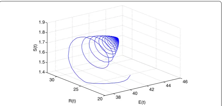
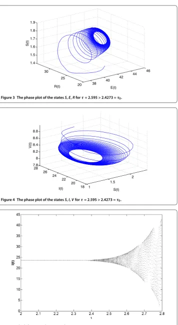
Fig-ures and ; it is easy to see that system () is asymptotically stable from FigFig-ures and . Then we chooseτ= . >τ. The corresponding phase plots are illustrated by Figures
and . We can see that system () undergoes a Hopf bifurcation in this case. This prop-erty can also be seen from the bifurcation diagram in Figure . In addition, we obtain
λ(τ) = . + .i,C() = –. + .i. Thus, we haveμ= . > ,
β= –. < ,T= –. < . From Theorem , we can conclude that the Hopf
bi-furcation is supercritical and the bifurcating periodic solutions are stable, and the period of the periodic solutions decreases.
5 Conclusions
Figure 3 The phase plot of the statesS,E,Rforτ= 2.595 > 2.4273 =τ0.
Figure 4 The phase plot of the statesS,I,Vforτ= 2.595 > 2.4273 =τ0.
for local stability of the positive equilibrium and existence of the Hopf bifurcation of sys-tem () are obtained. We have proven that when the conditions are satisfied, there exists a critical valueτof the delay below which system () is stable and above which system () is
unstable. Especially, system () undergoes a Hopf bifurcation at the positive equilibrium whenτ =τ. The occurrence of Hopf bifurcation means that the state of worms
preva-lence in a wireless sensor network changes from a positive equilibrium to a limit cycle, which is not welcomed in a wireless sensor network. Hence, we should control the occur-rence of Hopf bifurcation by combining some bifurcation control strategies, and we leave this as the future work. Further, the properties of Hopf bifurcation are studied by using the normal form method and the center manifold theorem. Finally, a numerical example is given to support our theoretical results.
Competing interests
The authors declare that they have no competing interests.
Authors’ contributions
All authors contributed equally to the writing of this paper. All authors read and approved the final manuscript.
Acknowledgements
The authors would like to thank the editor and the anonymous referees for their work on the paper. This work was supported by the Natural Science Foundation of Higher Education Institutions of Anhui Province (KJ2014A005).
Received: 30 September 2014 Accepted: 11 November 2014 Published:25 Nov 2014
References
1. Kephart, JO, White, SR: Measuring and modeling computer virus prevalence. In: IEEE Computer Security Symposium on Research in Security and Privacy, pp. 2-15. IEEE Press, New York (1993)
2. Kephart, JO, White, SR: Directed-graph epidemiological models of computer viruses. In: IEEE Symposium on Security and Privacy, pp. 343-361 (1991)
3. Yuan, H, Chen, G: Network virus epidemic model with the point-to-group information propagation. Appl. Math. Comput.206, 357-367 (2008)
4. Yang, LX, Yang, XF, Wen, LS, Liu, JM: A novel computer virus propagation model and its dynamics. Int. J. Comput. Math.89, 2307-2314 (2012)
5. Huang, CY, Lee, CL, Wen, TH, Sun, CT: A computer virus spreading model based on resource limitations and interaction costs. J. Syst. Softw.86, 801-808 (2013)
6. Mishra, BK, Pandey, SK: Fuzzy epidemic model for the transmission of worms in computer network. Nonlinear Anal., Real World Appl.11, 4335-4341 (2010)
7. Mishra, BK, Pandey, SK: Dynamic model of worms with vertical transmission in computer network. Appl. Math. Comput.217, 8438-8446 (2011)
8. Yang, LX, Yang, XF: Propagation behavior of virus codes in the situation that infected computers are connected to the Internet with positive probability. Discrete Dyn. Nat. Soc.2012, Article ID 693695 (2012)
9. Yang, MB, Zhang, ZF, Li, Q, Zhang, G: An SLBRS model with vertical transmission of computer virus over the Internet. Discrete Dyn. Nat. Soc.2012, Article ID 925648 (2012)
10. Yang, LX, Yang, XF, Zhu, QY, Wen, LS: A computer virus model with graded cure rates. Nonlinear Anal., Real World Appl.14, 414-422 (2013)
11. Mishra, BK, Pandey, SK: Dynamic model of worm propagation in computer network. Appl. Math. Model.38, 2173-2179 (2014)
12. Gan, CQ, Yang, XF, Liu, WP, Zhu, QY: A propagation model of computer virus with nonlinear vaccination probability. Commun. Nonlinear Sci. Numer. Simul.19, 92-100 (2014)
13. Akyildiz, I, Su, W, Sankarasubramaniam, Y, Cayirci, E: A survey on sensor networks. IEEE Commun. Mag.40, 102-114 (2002)
14. Mishra, BK, Keshri, N: Mathematical model on the transmission of worms in wireless sensor network. Appl. Math. Model.37, 4103-4111 (2013)
15. Feng, LP, Liao, XF, Li, HQ, Han, Q: Hopf bifurcation analysis of a delayed viral infection model in computer networks. Math. Comput. Model.56, 167-179 (2012)
16. Ren, JG, Yang, XF, Yang, LX, Xu, YH, Yang, FZ: A delayed computer virus propagation model and its dynamics. Chaos Solitons Fractals45, 74-79 (2012)
17. Dong, T, Liao, XF, Li, HQ: Stability and Hopf bifurcation in a computer virus model with multistate antivirus. Abstr. Appl. Anal.2012, Article ID 841987 (2012)
18. Hassard, BD, Kazarinoff, ND, Wan, YH: Theory and Applications of Hopf Bifurcation. Cambridge University Press, Cambridge (1981)
10.1186/1687-1847-2014-295
Cite this article as:Zhang and Si:Dynamics of a delayed SEIRS-V model on the transmission of worms in a wireless