A higher order blended compact difference (BCD) method for solving the general 2D linear second order partial differential equation

(1)

R E S E A R C H

Open Access

A higher-order blended compact difference

(BCD) method for solving the general 2D

linear second-order partial differential

equation

Tingfu Ma

1

_{and Yongbin Ge}

1*

*_{Correspondence:}_{[email protected]} 1_{Institute of Applied Mathematics} and Mechanics, Ningxia University, Yinchuan, China

Abstract

A higher-order blended compact difference (BCD) scheme is proposed to solve the general two-dimensional (2D) linear second-order partial differential equation. The distinguishing feature of the present method is that methodologies of explicit compact difference and implicit compact difference are blended together. Sixth-order accuracy approximations for the first- and second-order derivatives are employed, and the original equation is also discretized based on a 9-point stencil, which is different from the work of Lee et al. (J. Comput. Appl. Math. 264:23–37,2014). A truncation error analysis is performed to show that the scheme is of sixth-order accuracy for the interior grid points. Simultaneously, sixth-order accuracy schemes are proposed to compute the grid points on the boundaries for the first- and

second-order derivatives. Numerical experiments are conducted to demonstrate the accuracy and eﬃciency of the present method.

MSC: 65N06; 65N15; 65N22

Keywords: BCD scheme; Two-dimensional linear partial diﬀerential equation; Mixed derivative; Finite-diﬀerence method; Higher-order accuracy

1 Introduction

In this paper, we consider the general two-dimensional (2D) linear partial diﬀerential equation in the form

a(x,y)uxx+b(x,y)uyy+c(x,y)uxy+p(x,y)ux+q(x,y)uy+r(x,y)u=f(x,y). (1)

Here the unknown functionu, the variable coeﬃcient functionsa,b,c,p,q,r, and the forcing functionf are assumed to be continuously diﬀerentiable and have the required partial derivatives onΩ.Ωis a continuous rectangular domain. A suitable Dirichlet con-dition is prescribed on the boundary (∂Ω) in this paper.

Equation (1) is widely used in the fields of porous media flow [2,3] and when coordi-nate transformations are applied to a convection-diffusion equation on non-rectangular domains [4], which also generate Eq. (1). So it is both theoretically and practically im-portant to investigate their accurate, stable and efficient numerical methods. In the past

(2)

decades, high-order compact (HOC) difference methods have attracted increasing inter-ests for solving such equations [1,5–8]. The main feature of HOC methods is that they have higher-order accuracy (usually fourth-order, even higher) and higher spectral resolu-tion with relatively few grid points (compact grid stencil) than the convenresolu-tional difference methods. There are two kinds of compact difference methods. One is called the explicit compact difference method and the other is called the implicit compact difference method. For the explicit compact difference method, all the derivatives in partial differential equa-tions are explicitly approximated by the nodal values of the target function. Usually, 9 grid points are used for solving the 2D problems and no more than 27 grid points (usually 19 points) for solving the three-dimensional (3D) problems. For instance, in Ref. [9], Gupta et al. derived a fourth-order compact finite-difference scheme for the 2D convection-diffusion equation. Then they extended the method to the 2D elliptic equation without the mixed derivative term [5]. Karaa extended the work of Gupta et al. to the 2D elliptic and parabolic problems with mixed derivatives [8]. The basic idea of their methods lies in uti-lizing the Taylor expansions by 2D power series of all the functions involved in the differ-ential equation at the reference grid point (i,j), substituting these expansions into the orig-inal equation and comparing the coefficients ofxi_yj_{to get the linear constraints on the} un-known coefficients. In Ref. [8], the author considered the model equations with the mixed derivative terms, but the coefficients of the second derivativesuxxanduyy were equiva-lent to constants. In other words, if they are functions anda(x,y)=b(x,y), andc(x,y)= 0 in Eq. (1), there do not exist any explicit fourth-order compact difference schemes with 9-point grid stencil as was declared in Ref. [6]. And the authors of [6] also pointed out that explicit sixth-order compact difference schemes exist only ifa(x,y) =b(x,y) = 1,c(x,y) = 0, andp(x,y) =q(x,y). Special cases are the Poisson equation and the Helmholtz equation. Some fourth- and sixth-order compact difference schemes are reported in Refs. [10–16]. Additionally, some fourth-order compact difference schemes for the convection-diffusion equations and the steady incompressible Navier–Stokes equations are reported in Refs. [17–25].

(3)

As we discussed above, for the general 2D linear second-order equations with variable coefficients and the mixed derivative term like (1), it is impossible to get an explicit fourth-order compact difference scheme with 9 grid points except under certain conditions men-tioned above. But it is possible to get an implicit fourth-order, even sixth-order compact difference scheme for such equations with no more than 9 grid points. Very recently, Lee et al. [1] extended the work in [30] and proposed a combined compact difference (CCD2) scheme to solve Eq. (1). The highlight of this work is a sixth-order accurate difference scheme for the mixed derivative with a 9-point compact stencil at the interior region. It is a pity that just the fourth-order accuracy schemes on the boundaries are proposed in [1], which results in the convergence order of the CCD2 scheme is less than six for some problems. So, in this paper, we are aiming at developing a new sixth-order compact differ-ence scheme for solving the general 2D linear partial differential equation (1). Our method makes use of the explicit compact difference scheme in which the derivatives of the orig-inal differential equation are discretized and the implicit compact difference scheme in which all derivatives with their own schemes are involved in computation independently, which is named the blended compact difference (BCD) scheme. Namely, the original gov-erning equation is discretized with the 9-point compact stencil (like the explicit compact difference scheme) and a sixth-order compact difference scheme is proposed, but it still includes the representations of the first- and second-order derivatives (like the implicit compact difference scheme), which are computed by the sixth-order CCD schemes [30]. This scheme differs from the explicit compact difference method because the computa-tions of the first- and second-order derivatives are also needed in the scheme. And it also differs from the implicit CCD2 scheme [1] because the governing equation is required to be discretized simultaneously in the present method. Although the computational cost in-creases, it is more accurate and more convenient to conduct computation than the method described in [1,30]. We will illustrate this conclusion in the following sections.

This paper is organized as follows. In Sect.2, we present the method for deriving a sixth-order compact diﬀerence scheme for solving Eq. (1). Simultaneously, the sixth-order ac-curacy schemes are proposed to compute the grid points on the boundaries. In Sect.3, truncation error analysis is done to show that the scheme is sixth-order accuracy for the interior grid points. Next, numerical tests are conducted in Sect.4, and we compare the present scheme with other existing numerical methods in the literature. Finally, we give a brief conclusion in Sect.5.

2 Methodology of sixth-order BCD scheme

In this section, we brieﬂy discuss the development of BCD formulation for Eq. (1). Assume the problem domain to be rectangularΩ= [0,Lx]×[0,Ly], and we discrete the domain with uniform grids and sethxandhyto be the grid step-length in thex- andy-directions, respectively. The central mesh point (xi,yj) is denoted by 0 and the other 8 mesh points at (xi±hx,yj), (xi,yj±hy), (xi±hx,yj±hy), are denoted by numbers 1 – 8 (see Fig.1). For convenience, we denote the derivatives by{u,ux,uxx,uy,uyy,uxy}, respectively. We consider the general Dirichlet boundary condition. In the following sections, we will discuss how to implement the BCD scheme on a rectangular region.

2.1 Inner grid points

(4)

Figure 1Labeling of the 9 grid points

should provide 6 independent difference equations. Note that the original 3-point order CCD schemes for the first- and second-order derivatives as well as the 9-point sixth-order scheme of the mixed derivativeuxyare proposed in [30] and [1], respectively. We simply borrow the sixth-order schemes for the five derivatives {ux,uy,uxx,uyy,uxy} that are listed in Appendix1.

In order to get the BCD scheme, we use the Taylor series expansions at point (x,y).

ux=δxu– h2

x 6uxxx–

h4

x

120ux(5)+O

h6_x, (2)

uy=δyu–h

2

y 6uyyy–

h4

y

120uy(5)+O

h6_y. (3)

Hereδxandδy(see Appendix2) are standard central difference operators for the first-order derivatives. Substituting (2) and (3) into (1),we obtain the following modified differ-ential equation corresponding to Eq. (1):

auxx+buyy+cuxy+p

δxu– h2

x 6uxxx

+q

δyu– h2

y 6uyyy

+ru

– 1 120

ph4_xu_x(5)+qh4_yu_y(5)

+Oh6_x+h6_y=f. (4)

We now replace all the third-order derivatives in Eq. (4). Diﬀerentiating Eq. (1) with respect toxandy, respectively:

uxxx=

1

a(fx–buyyx–bxuyy–cuxxy–cxuxy–puxx–pxux–quyx–qxuy–rxu–rux)

–ax

a2(f–buyy–cuxy–pux–quy–ru)

, (5)

uyyy=

1

b(fy–auxxy–ayuxx–cuxyy–cyuxy–puxy–pyux–quyy–qyuy–ryu–ruy)

–by

b2(f –auxx–cuxy–pux–quy–ru)

. (6)

Substituting Eqs. (5)–(6) into Eq. (4),and rearranging it, we obtain

¯

(5)

+

(6)

+

Substituting the standard ﬁnite-diﬀerence operators (see Appendix 2) into (24) and omitting the truncation error terms, we obtain the following BCD scheme:

8

All the coeﬃcients are explicitly given as follows:

ˆ

(7)

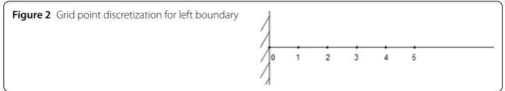
Figure 2Grid point discretization for left boundary

mixed second-order derivative uxy is approximated by the 9-point sixth-order interior

schemes (63) in Appendix 1. We now present some remarks on the BCD and CCD

schemes.

Remark1 The CCD scheme needs to couple all diﬀerence equations for the unknown function and its various derivatives together and solve them simultaneously along with

complex boundary schemes. It is unavoidable to result in large scale and complicated

co-eﬃcient matrix, which increases the complexity of algorithm design and programming. However, the BCD scheme is decoupled by means of solving the unknown function and its

various derivatives separately with an iteration process, so the derivation of the schemes,

the algorithm design and programming are simple and convenient to operate.

Remark2 The CCD scheme uses the original equation (1) as governing equation of the

unknown functionudirectly, while the BCD scheme uses the discretized equation, i.e., Eq. (25) to computeu. Obviously Eq. (25) is more complicated than the original

equa-tion (1), so the calculation cost correspondingly increases.

2.2 Boundary grid points

In the above section, we have developed diﬀerence equations for each interior grid point. Many applications involve computations in domains with non-periodic boundaries. In

this section, we will introduce approximations for the ﬁrst- and second-order derivatives

for the boundary nodes. For non-periodic problems, these approximations are, of neces-sity, non-central or one-sided. Additional sixth-order expressions are needed to compute

nodes at the boundaries nodes to close the system. Consider left boundary i= 0, the

sixth-order schemes of the ﬁrst-order derivative may be obtained from a relation of the form

(ux)0,j+α(ux)1,j= (b0u0,j+b1u1,j+b2u2,j+b3u3,j+b4u4,j+b5u5,j)/hx. (26)

The coeﬃcients b0,b1,b2,b3,b4,b5 (for the subscript see Fig.2) andα are derived by

(8)

are able to obtain the linear equations as shown below:

b0+b1+b2+b3+b4+b5= 0,

1 2!

b1+ 22b2+ 32b3+ 42b4+ 52b5

=α, 1

3!

b1+ 23b2+ 33b3+ 43b4+ 53b5

=α 2, 1

4!

b1+ 24b2+ 34b3+ 44b4+ 54b5

=α 6, 1

5!

b1+ 25b2+ 35b3+ 45b4+ 55b5

= α 24, 1

6!

b1+ 26b2+ 36b3+ 46b4+ 56b5

= α 120, 1

7!

b1+ 27b2+ 37b3+ 47b4+ 57b5

= α 720.

(27)

And resolving it by Matlab software, we can get the results as follows:

α= 5, b0= –

197

60 , b1= – 5

12, b2= 5,

b3= –

5

3, b4= 5

12, b5= – 1 20.

So, we can get the left boundary condition ofuxforj= 0, 1, . . . ,Ny:

(ux)0,j+ 5(ux)1,j=

–197 60u0,j–

5

12u1,j+ 5u2,j– 5 3u3,j+

5 12u4,j–

1

20u5,j hx. (28)

The derivation of the following boundary approximations for the ﬁrst-order and second-order derivatives is exactly analogous to the above process. The boundary schemes are summarized now.

Right boundary condition ofuxforj= 0, 1, . . . ,Ny:

(ux)Nx,j+ 5(ux)Nx–1,j=

197 60uNx,j+

5

12uNx–1,j– 5uNx–2,j+ 5 3uNx–3,j

– 5

12uNx–4,j+ 1

20uNx–5,j hx. (29)

Bottom boundary condition ofuyfori= 0, 1, . . . ,Nx:

(uy)i,0+ 5(uy)i,1=

–197 60 ui,0–

5

12ui,1+ 5ui,2– 5 3ui,3+

5 12ui,4–

1

20ui,5 hy. (30)

Top boundary condition ofuyfori= 0, 1, . . . ,Nx:

(uy)i,Ny+ 5(uy)i,Ny–1=

197 60ui,Ny+

5

12ui,Ny–1– 5ui,Ny–2+ 5 3ui,Ny–3

– 5

12ui,Ny–4+ 1

(9)

Left boundary condition ofuxxforj= 0, 1, . . . ,Ny:

(uxx)0,j– 6(uxx)1,j=

–403

18u0,j+ 33u1,j– 21

2 u2,j– 4

9u3,j h

2

x

+

–26

3 (ux)0,j– 6(ux)1,j+ 3(ux)2,j hx. (32)

Right boundary condition ofuxxforj= 0, 1, . . . ,Ny:

(uxx)Nx,j– 6(uxx)Nx–1,j=

–403

18uNx,j+ 33uNx–1,j– 21

2 uNx–2,j– 4

9uNx–3,j h

2

x

+

26

3 (ux)Nx,j+ 6(ux)Nx–1,j– 3(ux)Nx–2,j hx. (33)

Bottom boundary condition ofuyyfori= 0, 1, . . . ,Nx:

(uyy)i,0– 6(uyy)i,1=

–403

18ui,0+ 33ui,1– 21

2 ui,2– 4

9ui,3 h

2

y

+

–26

3(uy)i,0– 6(uy)i,1+ 3(uy)i,2 hy. (34)

Top boundary condition ofuyyfori= 0, 1, . . . ,Nx:

(uyy)i,Ny– 6(uyy)i,Ny–1=

–403

18 ui,Ny+ 33ui,Ny–1– 21

2 ui,Ny–2– 4

9ui,Ny–3 h

2

y

+

26

3 (uy)i,Ny+ 6(uy)i,Ny–1– 3(uy)i,Ny–2 hy. (35)

In the end, we will derive boundary conditions of the mixed derivative. We can regard the second mixed derivative uxyas the first partial derivative ofux (oruy) with respect toy(orx). Similar to the first-order derivative boundary scheme, by using the 2D Taylor expansions and some tedious calculations (see Appendix3), we are able to deduce some difference schemes for approximatinguxyfor grid points on the boundaries. A group of sixth-order accurate equations on the four boundaries can be given here.

Left boundary condition ofuxyforj= 0, 1, . . . ,Ny:

(uxy)0,j+ 1

5(uxy)1,j=

–149 60(uy)0,j+

1723

300(uy)1,j– 7(uy)2,j+ 19

3 (uy)3,j

–43 12(uy)4,j+

23 20(uy)5,j–

4

25(uy)6,j hx. (36)

Right boundary condition ofuxyforj= 0, 1, . . . ,Ny:

(uxy)Nx,j– 1

5(uxy)Nx–1,j=

29

12(uy)Nx,j– 1877

300 (uy)Nx–1,j+ 8(uy)Nx–2,j– 7(uy)Nx–3,j

+47

12(uy)Nx–4,j– 5

4(uy)Nx–5,j+ 13

(10)

Top boundary condition ofuxyfori= 0, 1, . . . ,Nx:

(uxy)i,Ny– 1

5(uxy)i,Ny–1=

29

12(ux)i,Ny– 1877

300 (ux)i,Ny–1+ 8(ux)i,Ny–2– 7(ux)i,Ny–3

+47

12(ux)i,Ny–4– 5

4(ux)i,Ny–5+ 13

75(ux)i,Ny–6 hy. (38)

Bottom boundary condition ofuxyfori= 0, 1, . . . ,Nx:

(uxy)i,0+

1

5(uxy)i,1=

–149 60(ux)i,0+

1723

300(ux)i,1– 7(ux)i,2+ 19

3 (ux)i,3

–43 12(ux)i,4+

23 20(ux)i,5–

4

25(ux)i,6 hy. (39)

With more than 4 grid points along one direction, the above boundary diﬀerence equa-tions are not strictly compact in the traditional sense, but they are necessary to retain the high-order accuracy of the BCD scheme. Nevertheless, we remark that these equations are only used for boundary grid points. The interior diﬀerence equations contribute to the major compact structure.

Note that if the Dirichlet boundary condition is replaced by the Neumann boundary condition, the equation (1) can also be solved because the functionuis unknown at the boundaries while the values of the ﬁrst-order derivativesuxanduyat the boundaries are known. According to Eqs. (28)–(31), the functionuat the boundaries can be calculated by the sixth-order schemes as follows:

u0,j= 60

–hx(ux)0,j– 5hx(ux)1,j– 5

12u1,j+ 5u2,j– 5 3u3,j+

5 12u4,j–

1

20u5,j 197, (40)

uNx,j= 60

hx(ux)Nx,j+ 5hx(ux)Nx–1,j– 5

12uNx–1,j+ 5uNx–2,j– 5 3uNx–3,j

+ 5

12uNx–4,j– 1

20uNx–5,j 197, (41)

ui,0= 60

–hy(uy)i,0– 5hy(uy)i,1–

5

12ui,1+ 5ui,2– 5 3ui,3+

5 12ui,4–

1

20ui,5 197, (42)

ui,Ny= 60

hy(uy)i,Ny+ 5hy(uy)i,Ny–1– 5

12ui,Ny–1+ 5ui,Ny–2– 5 3ui,Ny–3

+ 5

12ui,Ny–4– 1

20ui,Ny–5 197. (43)

2.3 Iterative procedure

The BCD scheme is decoupled by means of solving the unknown functionuand its various derivativesux,uy,uxx,uyy,uxyseparately with an iteration process. A pseudo code of the BCD scheme is listed as follows:

Give any initial guessu(0),u(0)x ,u(0)y ,u(0)xx,u(0)yy andu0xy Fork= 1, 2, . . .do

(11)

Computeu(yyk)by Scheme (62) in Appendix1and Schemes (34) and (35). Computeu(xyk)by Scheme (63) in Appendix1and schemes (36)–(39). Computeu(k)_{by Scheme (}₂₅₎

IfF–Lu(k)<ηis satisﬁed, then stop.

Herekis iteration number. L is the linear diﬀerence operator for representation of the scheme (25). · is a sort of norm.ηis the convergence tolerance.

3 Truncation error analysis

A brief truncation error analysis is given here. For the sake of simplicity, we suppose that hxandhyare equal toh, using the Taylor series expansions at point (x,y).

ux=δxu–h

2

6uxxx– h4

120ux(5)– h6

5040ux(7)+O

h8, (44)

uy=δyu–h

2

6uyyy– h4

120uy(5)– h6

5040uy(7)+O

h8. (45)

The original equation (1) is treated as an auxiliary relation that can be diﬀerentiated to yield expressions for the third-order derivatives,

uxxx=

1

a(fx–buyyx–bxuyy–cuxxy–cxuxy–puxx–pxux–quyx–qxuy–rxu–rux)

–ax

a2(f–buyy–cuxy–pux–quy–ru)

, (46)

uyyy=

1

b(fy–auxxy–ayuxx–cuxyy–cyuxy–puxy–pyux–quyy–qyuy–ryu–ruy)

–by

b2(f –auxx–cuxy–pux–quy–ru)

. (47)

Substituting Eqs. (44)–(47) into Eq. (1) and rearranging it,

¯

Auxx+Buyy¯ +Cuxy¯ +Dux¯ +Euy¯ +Guxyy¯ +Huxxy¯ +pδxu+qδyu –h

4_p

120ux(5)– h4_q

120uy(5)– h6

5040ux(7)– h6

5040uy(7)=F. (48)

¯

A,B¯,C¯,D¯,E¯,G¯,H¯ andFare deﬁned in Eqs. (8)–(15).

To obtain a sixth-order compact formulation for Eq. (48), consider the following approx-imations for all the derivatives:

uxx= 2δ2_xu–δxux+ h

4

360ux(6)+ h6

10,080ux(8)+O

h8, (49)

uyy= 2δ2_yu–δyuy+ h

4

360uy(6)+ h6

10,080uy(8)+O

h8, (50)

uxxy=δ_x2uy+δ_x2δyu–δxδyux+ h4

36ux4y3+O

h6, (51)

uyyx=δ_y2ux+δ_y2δxu–δxδyuy+ h4

36uy4x3+O

h6, (52)

u_x(5)= 360 7h4

ux–δxu+ h2

6 δxuxx

–3h

2

49ux(7)+O

(12)

u_y(5)=

Notice that all the derivatives ux,uxx,uy,uyy,uxy are calculated independently by the formulas (76)–(80) in Appendix4. Substituting their truncation error –h6

7!ux(7), –2h

Truncation =h

6

4 Numerical experiments

In this section, we conduct numerical experiments with three test problems chosen from the literature to test the high-order accuracy of the BCD scheme. All problems are de-ﬁned on the unit square domainΩ= (0, 1)×(0, 1). For all three problems, the right-hand functionsf and the Dirichlet boundary conditions are prescribed to satisfy the given ana-lytic solution. We select the hybrid biconjugate gradient stabilized method (BiCGStab(2)) [44] to solve the resulting linear systems in all test problems. All iterative procedures are started with zero initial guesses and are terminated when the Euclidean norm of the resid-ual vector is reduced by 1010_{. The code is written in Fortran 77 programming language}

(13)

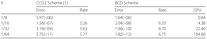
Table 1 The maximum absolute error and convergence rate of diﬀerent discretization for Problem 1

h CCD2 Scheme [1] BCD Scheme

Error Rate Error Rate CPU

1/8 5.97(–06) 1.64(–06) 0.84

1/16 1.56(–07) 5.26 2.04(–08) 6.33 4.38

1/32 3.14(–09) 5.63 1.96(–10) 6.70 22.40

1/64 5.75(–11) 5.77 1.82(–12) 6.75 104.80

the convergence rate of the method are computed with the following deﬁnition:

Error =max

i,j ui,j–u(xi,yj); Rate =

log(Error1/Error2)

log(h1/h2)

,

whereu(xi,yj) is the exact solution. Error1 and Error2 are the maximum absolute errors estimated for the two diﬀerent grid step sizesh1andh2.

4.1 Problem 1: With variable coefﬁcients [1,45]

Consider the following diﬀerential equation in the presence of a source term:

(x+ 1)2+y2uxx– 2xyuxy+ (x+ 1)2uyy+ (x+ 2)ux–yuy=f(x,y).

The analytic solution is

u=x3y2+xsin(x)cos(xy).

We notice that Problem 1 has a non-periodic boundary condition. For comparison, the results of the CCD2 scheme [1] are also given. Firstly, we use diﬀerent mesh sizes from 1/8 to 1/64 to evaluate the computed accuracy order. Table1gives the maximum absolute errors and the convergence rate for Problem 1. We can clearly see that the BCD scheme obtains sixth-order accuracy and gets a more accurate solution than the CCD2 scheme. The CCD2 scheme cannot reach sixth-order accuracy because the fourth-order scheme is used for the boundaries computation, which inﬂuences the whole computed accuracy.

4.2 Problem 2: With high anisotropy ratio [1]

εx2+y2uxx+ 2(ε– 1)xyuxy+x2+εy2uyy+ (3ε– 1)xux+ (3ε– 1)yuy=f(x,y). The analytic solution is

u=sin(πx)sin(πy).

The second model problem is an anisotropy problem.εis chosen to reﬂect the mag-nitude of the anisotropy. Note thatε= 1 gives an isotropic equation, and the degree of anisotropy increases whenεbecomes smaller. The maximum absolute errors, the conver-gence rate and CPU time forε= 10–1_{and 10}–3_{, using CCD2 scheme and the BCD scheme,}

(14)

Table 2 The maximum absolute error and convergence rate for Problem 2 withε= 10–1

1/8 1.27(–04) 4.72(–05) 0.37

1/16 1.09(–06) 6.87 5.73(–07) 6.36 1.37

1/32 8.71(–09) 6.96 5.24(–09) 6.77 7.67

1/64 6.87(–11) 6.99 4.89(–11) 6.74 40.27

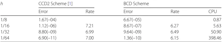
Table 3 The maximum absolute error and convergence rate for Problem 2 withε= 10–3

1/8 1.67(–04) 6.67(–05) 0.87

1/16 1.12(–06) 7.21 8.67(–07) 6.27 5.63

1/32 8.80(–09) 6.99 9.64(–09) 6.49 50.90

1/64 6.90(–11) 7.00 1.36(–10) 6.15 398.46

absolute errors of the BCD scheme and the CCD2 scheme are almost identical. They are seventh-order accurate and their excellent performances are obviously independent of the anisotropy ratioε= 10–1 andε= 10–3. Whenε= 10–1, the BCD scheme yields a slightly better solution than the CCD2 scheme. However, whenε= 10–3, the CCD2 scheme gets a slightly better solution than the BCD scheme. We notice that values on the boundaries are zero (periodic boundary conditions), for the CCD2 scheme, the fourth-order scheme for periodic boundary conditions does not inﬂuence the results of inner grid points.

In Table2and Table3it can be shown that the CPU time is related to the number of grid points and anisotropy ratio. We ﬁnd the same anisotropy ratio in which the number of grid points becomes higher when the CPU time is higher and the same number of grid points with which anisotropy ratio is higher when the CPU time is higher.

4.3 Problem 3: With large Reynold number [1,8]

uxx+cos(πx)sin(πy)uxy+uyy–Re(1 –x)(1 – 2y)ux+ 4Rexy(1 –y)uy=f(x,y). The analytic solution is

u=sin(πx) +sin(πy) +sin(πx)sin(πy).

For comparison, we use the BCD, the FOC [8], and the CCD2 schemes [1] to compute the numerical solutions of Problem 3.

Tables4–6give the maximum absolute errors, the convergence rate and CPU time, when

Re= 102_{, 10}4_{, 10}6_{, respectively. It is seen that the BCD and CCD2 schemes are almost not}

(15)

Table 4 The maximum absolute error and convergence rate for Problem 3 with Re = 102

h FOC scheme [8] CCD2 scheme [1] BCD scheme

Error Rate Error Rate Error Rate CPU

1/8 8.56(–03) 3.93(–04) 9.06(–05) 0.39

1/16 6.49(–04) 3.72 3.08(–06) 7.19 1.19(–06) 6.25 1.48

1/32 4.09(–05) 3.99 2.11(–08) 7.16 1.07(–08) 6.80 7.69

1/64 2.56(–06) 4.00 1.48(–10) 6.99 8.74(–11) 6.94 47.71

Table 5 The maximum error and convergence rate for Problem 3 with Re = 104

1/8 1.50(–02) 4.17(–04) 7.80(–05) 0.94

1/16 4.89(–03) 1.62 4.38(–06) 6.57 1.01(–06) 6.27 4.03

1/32 1.74(–03) 1.49 3.84(–08) 6.84 9.11(–09) 6.79 29.42

1/64 2.81(–04) 2.63 3.28(–10) 6.87 7.78(–11) 6.87 119.64

Table 6 The maximum error and convergence rate for Problem 3 with Re = 106

1/8 1.50(–02) 4.16(–04) 7.78(–05) 0.97

1/16 4.82(–03) 1.63 4.29(–06) 6.60 1.01(–06) 6.27 4.25

1/32 1.84(–03) 1.39 3.55(–08) 6.92 9.02(–09) 6.81 40.28

1/64 6.21(–04) 1.56 2.87(–10) 6.95 7.37(–11) 6.94 211.16

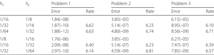
Table 7 The maximum error and convergence rate for Problem 1, Problem 2 withε= 10–1and Problem 3 with Re = 10

hx hy Problem 1 Problem 2 Problem 3

Error Rate Error Rate Error Rate

1/16 1/8 1.84(–08) 3.85(–05) 6.15(–05)

1/32 1/16 1.87(–10) 6.62 5.14(–07) 6.23 8.95(–07) 6.10

1/64 1/32 1.88(–12) 6.63 4.80(–09) 6.74 8.56(–09) 6.71

1/8 1/16 1.76(–06) 3.85(–05) 6.27(–05)

1/16 1/32 2.09(–08) 6.40 5.14(–07) 6.23 7.47(–07) 6.39

1/32 1/64 2.97(–10) 6.14 4.59(–09) 6.81 7.85(–09) 6.57

Finally, the maximum absolute error and the convergence rate of Problem 1, Problem 2 withε= 10–1_{and Problem 3 with}_Re_{= 10 are given in Table}₇_when_hx_{is not equal to}_hy_.

Numerical results also show that the BCD scheme can reach its theoretical sixth-order accuracy.

5 Conclusions

(16)

large ﬁrst derivative terms or anisotropy problems. (ii) We perform a sixth-order compu-tation for the grid points on the boundaries, while Ref. [1] uses the fourth-order scheme, which decreases the accuracy order of solution for those problems with non-periodic boundary conditions. (iii) Our method is decoupled, i.e., we can solve the unknown func-tionuand its various derivatives separately with an iteration process. Its advantage is that the derivation of the scheme, the algorithm design and programming are simple and easy to operate in the extension to high-dimensional problems. Especially for the problems of complex ﬂow and heat transfer, it is relatively easy to construct a discrete scheme with high precision and for their boundary conditions. Numerical experiments are conducted to demonstrate the accuracy of the present scheme. It is shown that the present method is more accurate than those in the literature.

Appendix 1: The sixth-order schemes of the ﬁrst- and second-order derivatives as well as the mixed derivative

For the ﬁrst- and second-order derivatives along thex- andy-directions [30]

7

16ux1+ux0+ 7 16ux3=

15

16hxu1–u3) + hx

16(uxx1–uxx3) +O

h6_x, (59)

–1

8uxx1+uxx0– 1 8uxx3=

3 h2

x

(u1– 2u0+u3) –

9

8hx(ux1–ux3) +O

h6_x, (60)

7

16uy2+uy0+ 7 16uy4=

15

16hy(u2–u4) + hy

16(uyy2–uyy4) +O

h6_y, (61)

–1

8uyy2+uyy0– 1 8uyy4=

3 h2

y

(u2– 2u0+u4) –

9

8hy(uy2–uy4) +O

h6_y. (62)

For the mixed derivativeuxy[1]

(uxy)0+

1 16

₄

i=1

(uxy)i

– 1 32

₈

i=5

(uxy)i

= 9 16hy

(ux)2– (ux)4

+ 9 16hx

(uy)1– (uy)3

– 9

32hxhy(u5–u6+u7–u8) + h6

x

960ux(5)y(3)+ h6

y

960ux(3)y(5)+O

h8_x+h8_y. (63)

Appendix 2: Details of the central difference operators

δ2_xu0=

u1– 2u0+u3

h2

x

; δxu0=

u1–u3

2hx ,

δ2_yu0=

u2– 2u0+u4

h2

y

; δyu0=

u2–u4

2hy ,

δ2_xδyu0=

u5+u6–u7–u8– 2u2+ 2u4

2h2

xhy

,

δ2_yδxu0=

u5–u6–u7+u8– 2u1+ 2u3

2h2

yhx

(17)

δxδyu0=

u5–u6+u7–u8

4hxhy .

Appendix 3: The sixth-order schemes of the mixed derivative on the boundaries

The sixth-order scheme of left boundary of the mixed derivative may be obtained from a relation of the form

(uxy)0,j+α(uxy)1,j=

α are derived by matching the Taylor series coeﬃcients of various orders. The detailed derivation process is given here.

Using the Taylor series expansions at point (0,j)

(18)

and substituting Eqs. (65)–(70) into Eq. (64), we are able to obtain linear equations as shown below:

a0+a1+a2+a3+a4+a5+a6= 0,

1 2!

a1+ 22a2+ 32a3+ 42a4+ 52a5+ 62a6

=α, 1

3!

a1+ 23a2+ 33a3+ 43a4+ 53a5+ 63a6

=α 2, 1

4!

a1+ 24a2+ 34a3+ 44a4+ 54a5+ 64a6

=α 6, 1

5!

a1+ 25a2+ 35a3+ 45a4+ 55a5+ 65a6

= α 24, 1

6!

a1+ 26a2+ 36a3+ 46a4+ 56a5+ 66a6

= α 120, 1

7!

a1+ 27a2+ 37a3+ 47a4+ 57a5+ 67a6

= α 720.

(71)

Resolving it by Matlab software, we can get the results as follows:

α=1

5, a0= – 149

60, a1= 1723

300 , a2= –7, a3= 19

3 ,

a4= –

43

12, a5= 23

20, a6= – 4 25.

So, the sixth-order scheme for the left boundary of the mixed derivative can be written as

(uxy)0,j+ 1 5(uxy)1,j

=

–149 60(uy)0,j+

1723

300 (uy)1,j– 7(uy)2,j+ 19

3 (uy)3,j– 43 12(uy)4,j

+23 20(uy)5,j–

4

25(uy)6,j hx. (72)

The derivation of right boundary scheme for the mixed derivative is exactly analogous to the left boundary. The right boundary scheme is summarized below:

(uxy)Nx,j– 1

5(uxy)Nx–1,j

=

29

12(uy)Nx,j– 1877

300 (uy)Nx–1,j+ 8(uy)Nx–2,j– 7(uy)Nx–3,j

+47

12(uy)Nx–4,j– 5

4(uy)Nx–5,j+ 13

75(uy)Nx–6,j hx, j= 0, 1, 2, . . . ,Ny. (73)

In the same way, we can get the sixth-order schemes for approximating the top and bottom boundaries as follows:

(uxy)i,Ny– 1

(19)

=

Appendix 4: The truncation errors of the sixth-order schemes of the ﬁrst- and second-order derivatives and the mixed derivative

7

The authors would like to thank the editors and the referees, whose constructive comments were helpful in improving the quality of this paper.

Funding

This work was supported in part by the National Natural Science Foundation of China under Grants 11772165 and 11361045, and the National Natural Science Foundation of Ningxia under Grant 2018AAC02003, and the Key Research and Development Program of Ningxia under Grant 2018BEE03007.

Availability of data and materials Not applicable.

Competing interests

The authors declare that they have no competing interests.

Authors’ contributions

YG deﬁned the research theme. TM designed numerical method and conducted numerical experiments. YG interpreted the results and wrote the paper. All author have seen and approved the ﬁnal version of the manuscript.

Publisher’s Note

(20)

Received: 3 September 2018 Accepted: 20 February 2019 References

1. Lee, S.T., Liu, J., Sun, H.W.: Combined compact diﬀerence scheme for linear second-order partial diﬀerential equations with mixed derivative. J. Comput. Appl. Math.264, 23–37 (2014)

2. Arbogast, T., Wheeler, M., Yotov, I.: Mixed finite elements for elliptic problems with tensor coefficients as cell-centered finite differences. SIAM J. Numer. Anal.34, 828–852 (1997)

3. Friis, H., Edwards, M., Mykkeltveit, J.: Symmetric positive definite flux-continuous full-tensor finite-volume schemes on unstructured cell-centered triangular grids. SIAM J. Sci. Comput.31, 1192–1220 (2008)

4. Ge, L., Zhang, J.: High accuracy iterative solution of convection diﬀusion equation with boundary layers on nonuniform grids. J. Comput. Phys.171, 560–578 (2001)

5. Gupta, M.M., Manohar, R.P., Stephenson, J.W.: High-order diﬀerence schemes for two- dimensional elliptic equations. Numer. Methods Partial Diﬀer. Equ.1, 71–80 (1985)

6. Ananthakrishnaiah, U., Manohar, R., Stephenson, J.W.: High-order methods for elliptic equation with variable coeﬃcients. Numer. Methods Partial Diﬀer. Equ.3, 219–227 (1987)

7. Gordin, V.A., Tsymbalov, E.A.: Compact diﬀerence scheme for parabolic and Schrödinger-type equations with variable coeﬃcients. J. Comput. Phys.375, 1451–1468 (2018)

8. Karaa, J.S.: High-order diﬀerence schemes for 2D elliptic and parabolic problems with mixed derivatives. Numer. Methods Partial Diﬀer. Equ.23, 366–378 (2007)

9. Gupta, M.M., Manohar, R.P., Stephenson, J.W.: A single cell high order scheme for the convection-diﬀusion equation with variable coeﬃcients. Int. J. Numer. Methods Fluids4, 641–651 (1984)

10. Gupta, M.M.: A fourth order Poisson solver. J. Comput. Phys.55, 166–172 (1984)

11. Spotz, W.F., Carey, G.F.: A high-order compact formulation for the 3D Poisson equation. Numer. Methods Partial Diﬀer. Equ.12, 235–243 (1996)

12. Gupta, M.M., Kouatchou, J.: Symbolic derivation of finite difference approximations for the three-dimensional Poisson equation. Numer. Methods Partial Differ. Equ.14, 593–606 (1998)

13. Wang, J., Zhong, W., Zhang, J.: A general meshsize fourth-order compact diﬀerence discretization scheme for 3D Poisson equation. Appl. Math. Comput.183, 804–812 (2006)

14. Sutmann, G., Steﬀen, B.: High-order compact solvers for the three-dimensional Poisson equation. J. Comput. Appl. Math.187, 142–170 (2006)

15. Singer, I., Turkel, E.: Sixth-order accurate ﬁnite diﬀerence schemes for the Helmholtz equation. J. Comput. Acoust.14, 339–351 (2006)

16. Turkel, E., Gordon, D., Gordon, R., Tsynkov, S.: Compact 2D and 3D sixth order schemes for the Helmholtz equation with variable wave number. J. Comput. Phys.232, 272–287 (2013)

17. Dennis, S.C.R., Hudson, J.D.: Compact ﬁnite diﬀerence approximation to operators of Navier–Stokes type. J. Comput. Phys.85, 390–416 (1989)

18. Chen, G.Q., Gao, Z., Yang, Z.F.: A perturbational h4 exponential finite difference scheme for the convective diffusion equation. J. Comput. Phys.104, 129–139 (1993)

19. Radhakrishna Pillai, A.C.: Fourth-order exponential finite difference methods for boundary value problems of convection diffusion type. Int. J. Numer. Methods Fluids37, 87–106 (2001)

20. Zhang, J., Sun, H.W., Zhao, J.J.: High order compact scheme with multigrid local mesh reﬁnement procedure for convection diﬀusion problems. Comput. Methods Appl. Mech. Eng.191, 4661–4674 (2002)

21. Zhang, J.: An explicit fourth-order compact finite difference scheme for three dimensional convection-diffusion equation. Commun. Numer. Methods Eng.14, 263–280 (1998)

22. Tian, Z.F., Dai, S.Q.: High-order compact exponential finite difference methods for convection-diffusion type problems. J. Comput. Phys.220, 952–974 (2007)

23. Spotz, W.F., Carey, G.F.: High-order compact scheme for the steady stream-function vorticity equations. Int. J. Numer. Methods Eng.38, 3497–3512 (1995)

24. Li, M., Tang, T., Fornberg, B.: A compact fourth-order ﬁnite diﬀerence scheme for the steady incompressible Navier–Stokes equations. Int. J. Numer. Methods Fluids30, 1137–1151 (1995)

25. Tian, Z.F., Ge, Y.B.: A fourth-order compact finite difference scheme for the steady stream function vorticity formulation of the Navier–Stokes/Boussinesq equations. Int. J. Numer. Methods Fluids41, 495–518 (2003) 26. Kreiss, H.O., Orszag, S.A., Israeli, M.: Numerical simulation of viscous incompressible flow. Annu. Rev. Fluid Mech.6,

281–318 (1974)

27. Hirsh, R.S.: Higher order accurate difference solutions of fluid mechanics problems by a compact differencing technique. J. Comput. Phys.19, 90–109 (1975)

28. Adam, Y.: A Hermitian ﬁnite diﬀerence method for the solution of parabolic equations. Comput. Math. Appl.1, 393–406 (1975)

29. Lele, S.K.: Compact finite difference schemes with spectral-like resolution. J. Comput. Phys.103, 16–42 (1992) 30. Chu, P.C., Fan, C.W.: A three-point combined compact difference scheme. J. Comput. Phys.140, 370–399 (1998) 31. Fu, D.X., Ma, Y.W., Liu, H.: Upwind compact scheme and application. In: Proceedings of the 5th International

Symposium on Computational Fluid Dynamics, vol. 1, pp. 184–190 (1993)

32. Deng, X.G., Zhang, H.X.: Developing high-order accurate weighted compact nonlinear scheme. J. Comput. Phys.165, 22–44 (2000)

33. Jiang, L., Shan, H., Liu, C.: Weighted compact scheme for shock capturing. Int. J. Comput. Fluid Dyn.15, 147–155 (2001)

34. Zhong, X., Tatineni, M.: High-order non-uniform grid schemes for numerical simulation of hypersonic boundary-layer stability and transition. J. Comput. Phys.190, 419–458 (2003)

35. Capdeville, G.: A central WENO scheme for solving hyperbolic conservation laws on non-uniform meshes. J. Comput. Phys.227, 2977–3014 (2008)

(21)

37. Xie, S.S., Yi, S.C., Kwon, T.I.: Fourth-order compact diﬀerence and alternating direction implicit schemes for telegraph equations. Comput. Phys. Commun.183, 552–569 (2012)

38. Liu, X., Zhang, S., Zhang, H., Chi, W.: A new class of central compact schemes with spectral-like resolution I: linear schemes. J. Comput. Phys.248, 235–256 (2013)

39. Liao, H.L., Sun, Z.Z.: A two-level compact ADI method for solving second-order wave equations. Int. J. Comput. Math. 90, 1471–1488 (2013)

40. Mingham, C.G., Causon, D.M.: A simple high-resolution advection scheme. Int. J. Numer. Methods Fluids56, 469–484 (2008)

41. Tian, Z.F., Liang, X., Yu, P.X.: A higher order compact ﬁnite diﬀerence algorithm for solving the incompressible Navier–Stokes equations. Int. J. Numer. Methods Eng.88, 511–532 (2011)

42. Qin, Q., Xia, Z.A., Tian, Z.F.: High accuracy numerical investigation of double-diﬀusive convection in a rectangular enclosure with horizontal temperature and concentration gradients. Int. J. Heat Mass Transf.71, 405–423 (2014) 43. Zhao, B.X., Tian, Z.F.: High-resolution high-order upwind compact scheme-based numerical computation of natural

convection ﬂows in a square cavity. Int. J. Heat Mass Transf.98, 313–328 (2016) 44. Kelly, C.T.: Iterative Methods for Linear and Nonlinear Equations. SIAM, Philadelphia (1995)