Curved beam elasticity theory based on the displacement function method using a finite difference scheme

(1)

R E S E A R C H

Open Access

Curved beam elasticity theory based on the

displacement function method using a ﬁnite

difference scheme

Wankui Bu

1*

_{and Hui Xu}

1

*_{Correspondence:} [email protected]

1_{College of Urban Construction,}

Heze University, Heze City, China

Abstract

A displacement function suitable for plane curved beam in polar coordinates is introduced, and a partial differential governing equation of plane curved beam is obtained by theoretical analysis. Then, the formulation of displacement components and stress components is expressed by the displacement function. On this basis, a finite difference scheme of the partial differential governing equation, displacement components, and stress components of an elastic body in polar coordinates is presented. Finally, the finite difference equations of theoretical formulation are applied to analyze the stress distribution of curved rock, which will provide scientific basis and reference for coal mining engineering.

Keywords: Displacement function; Elastic theory of curved beam; Finite diﬀerence

method; Curved rock

1 Introduction

The stress function method has been successfully applied to solve curved beam problems in the theory of elasticity, such as the Lame solution of the ring or cylinder subjected to the uniform pressure, the Guo solution of the curved beam bearing bending moment [1–7], the Kirs solution of the stress concentration at the edge of circular hole, the Mitchell solu-tion and the Gris solusolu-tion and Li solusolu-tion for the wedge body bearing surface force, and the Flamant solution of the semi-planar body subjected to concentrated force on the bound-ary [8–15]. The application of the stress function method has achieved certain results. The stress function can be obtained by solving the compatible equation for the axisymmetric problem or the simple non-axisymmetric problem [16–19]; however, the boundary condi-tion can only be in terms of loading condicondi-tions. When the boundary restraint is in terms of radial or circumferential displacement/strain conditions, the stress function method can-not obtain satisfactory solution. On the other hand, the direct displacement parameters method involves finding two displacement parameters (radial displacement and circum-ferential displacement) from two partial differential equilibrium equations. However, it is very difficult to obtain two displacement parameters from two second order partial differ-ential equations with variable coefficients, especially when the boundary conditions are in terms of mixed boundary with restrains and loadings. In practical applications, most practical problems with mixed boundary-value type are mainly accomplished by

(2)

cal calculation. The finite element method (FEM) and the finite difference method (FDM) are the major numerical methods. The FEM has been widely used in many fields, especially in the curve structure [20–23]. Gangan pointed out that the calculation error of a finite element will increase with the increase of flexure deformation [24]. It has been proved that the accuracy of FDM in stress analysis of structural members is higher than that of FEM [25,26].

The displacement function suitable for curved beam with mixed boundary conditions in polar coordinates, which is defined in terms of radial and circumferential displacement components, is introduced in the present paper. Moreover, the partial differential govern-ing equation of curved beam and the expression of displacement components and stress components are obtained in terms of displacement function. On this basis, the finite dif-ference scheme of partial differential governing equation, displacement components, and stress components of elastic body in polar coordinates is presented. Finally, the finite dif-ference equations of theoretical formulation are applied to analyze the stress distribution of curved rock.

2 Governing equations expressed by displacement components

With the elastic theory to a polar coordinate system (r,θ), the equilibrium equations for isotropic materials in terms of stress componentsσr,σθ, andτrθunder plane strain con-ditions in the absence of body force are as follows:

∂σr

For the plane strain, the stress components can be expressed as [1,2]

σr=

whereEandμare the elastic modulus and Poisson’s ratio of the material, respectively. Taking the plane strain case as an example, the stress component expressions (2a)–(2c) are substituted into Eqs. (1a)–(1c), and the formulations are obtained as follows:

(3)

∂3_u

∂θ3 are obtained.

∂3_u the governing equations for solving the plane elasticity problem with displacement com-ponents in polar coordinates. The solution satisfying both Eqs. (3a), (3b) and boundary conditions should be the exact solution. However, Eqs. (3a) and (3b) are elliptic partial dif-ferential equations with variable coeﬃcients. At the same time, boundary conditions are often mixed modes of stress and displacement boundary conditions. Therefore, the exact solution to this problem is not always an easy task theoretically. An alternative mathemat-ical method is transforming the terms of two variables in partial diﬀerential equations into a single variable with all possible modes of boundary conditions.

3 Governing equations expressed by displacement function

(4)

Substituting Eqs. (5a) and (5b) into Eqs. (3a) and (3b), the governing equations expressed by the displacement function are given as follows:

(5)

Here, for solving the variable ψ(r,θ) with two governing equations, it is necessary to determine some coeﬃcientsαi(i= 1, 2, 3, . . . , 12) reasonably that make one of the two

gov-erning equations redundant. Mathematically, it is required that one equation of Eqs. (6a)– (6b) can be satisﬁed under all circumstances. However, it is obvious that all the partial derivatives of the displacement functionψ(r,θ) as well as itself cannot be vanished only when the coeﬃcients of all the derivatives ofψ(r,θ) as well as itself are zero.

3.1 Governing equation—Form I

It is assumed that Eq. (6a) is satisfied automatically, and Eq. (6b) is the governing equation in terms of the displacement functionψ(r,θ). Let the coefficients ofψ(r,θ) as well as all its derivatives in Eq. (6a) equate to zero, the coefficientsαi(i= 1, 2, 3, . . . , 12) are obtained

as follows:

αi= 0 (i= 1, 3, 4, 6, 8, 11), (7a)

α2= –

1

2(1 –μ), (7b)

α5=

(5 – 4μ)

2(1 –μ), (7c)

α7= 1, (7d)

α9=

(1 – 2μ)

2(1 –μ), (7e)

α10= –3, (7f)

α12= 3. (7g)

And the governing equation in terms of the displacement functionψ(r,θ) is ∂4_ψ

∂r4 +

1

r4 ∂4_ψ

∂θ4 +

2

r2 ∂4_ψ ∂r2_∂θ2 –

2

r

∂3_ψ ∂r3 –

6

r3 ∂3_ψ ∂r∂θ2+

5

r2 ∂2_ψ

∂r2 +

10

r4 ∂2_ψ

∂θ2

– 9

r3 ∂ψ

∂r +

9

r4ψ= 0. (8)

Equation (8) gives the exact expression of the governing equation of the displacement function for the plane elastic problem in polar coordinates. It is not diﬃcult to conclude that the displacement function governing equation is a partial diﬀerential equation that is independent of the material constants such as elastic modulusEand Poisson’s ratioμ.

3.2 Governing equation—Form II

It is assumed that Eq. (6b) is satisfied automatically, and Eq. (6a) is the governing equation in terms of the displacement functionψ(r,θ). Let the coefficients ofψ(r,θ) as well as all its derivatives in Eq. (6b) equate to zero, the coefficientsαi(i= 1, 2, 3, . . . , 12) are obtained

as follows:

αi= 0 (i= 2, 5, 7, 9, 10, 12), (9a)

α1= –

(1 – 2μ)

(6)

α3= –

And the control equation in terms of the displacement functionψ(r,θ) is

∂4ψ

It is obvious that the partial diﬀerential equations in terms of displacement function given by Eq. (8) and (10) are identical, that is, the displacement function governing

equa-tions I and II are the same equation. That is, the governing equation expressed by the displacement functionψ(r,θ) is unique.

4 Displacement components and stress components expressed by displacement function

To solve the displacement function governing Eqs. (8) or (10), it is necessary to know the displacement boundary conditions or stress boundary conditions at each point on the boundary. However, the displacement boundary conditions of the elastic body are of-ten known displacements, and the stress boundary conditions are ofof-ten known loadings. Therefore, it is necessary to express the known displacement components and stress com-ponents as the partial derivative in terms of the displacement functionψ(r,θ).

The displacement components of the plane strain problem in polar coordinates are the radial displacementur(r,θ) and the circumferential displacementuθ(r,θ), and the stress components are the radial stressσr, the circumferential stressσθ, and the shear stressτrθ.

Equations (5a)–(5b) is substituted into Eqs. (2a)–(2c), the stress components are ex-pressed by the displacement function as follows in the case of plane strain:

(7)

σθ= E(1 –μ)

4.1 Displacement and stress expressions—Form I

Substituting the values ofαiin Eqs. (7a)–(7g) into Eqs. (5a)–(5b), the displacement

com-ponents expressions are as follows:

ur(r,θ) = –

nents expressions are as follows:

σr=

4.2 Displacement and stress expressions—Form II

Substituting the values ofαiin Eqs. (9a)–(9g) into Eqs. (5a)–(5b), the displacement

com-ponents expressions are as follows:

ur=

nents expressions are as follows:

(8)

σθ= E(1 –μ)

5 Finite difference scheme

In this section, the finite difference method is used to obtain the numerical solution of nodal values of the displacement function satisfying the governing equation. It is obvious that the governing equation in terms of the displacement function is a fourth-order ellip-tical partial differential equation with variable coefficients. At the same time, the stress expression expressed in terms of the displacement function is a third-order partial differ-ential equation, and the displacement expression expressed in terms of the displacement function is a second-order partial differential equation.

All of these partial differential equations are transformed into their corresponding alge-braic equations by using the finite difference method. The numerical calculation process is divided into three steps: Firstly, the values of the displacement function at each point of the domain are solved by the algebraic equations of the governing equations and the boundary conditions. Secondly, the partial derivative values of the displacement functions at each point are obtained by their difference equations. Finally, the displacement components and the stress components at each point are solved by the partial derivative values of the displacement function and the values of the displacement function.

5.1 Difference scheme of governing equation

The governing equation in terms of displacement function is suitable for solving the inter-nal mesh points of the domain. According to Eq. (8), the governing equation is composed of total eight diﬀerent partial derivatives of the displacement function of order ranging from one to four together with the displacement function itself. All the individual deriva-tives of the governing equation are replaced by their corresponding central diﬀerence ex-pressions having local truncation errors ofo(h2_{) and}_o₍_k2_{). The mesh length in}_r_-direction

(9)

∂2_ψ ∂r2

i,j

= 1

h2[ψi+1,j– 2ψi,j+ψi–1,j], (16f)

∂2ψ ∂θ2

i,j

= 1

k2[ψi,j+1– 2ψi,j+ψi,j–1], (16g)

∂ψ ∂r

i,j

= 1

2h[ψi+1,j–ψi–1,j]. (16h)

Substituting Eqs. (16a)–(16h) into Eq. (8), the governing equation for solving the internal mesh points of the domain is written in terms of nodal unknowns of the displacement functionψas follows:

ξ1ψ(i+ 2,j) +ξ2ψ(i+ 1,j+ 1) +ξ3ψ(i+ 1,j) +ξ2ψ(i+ 1,j– 1) +ξ4ψ(i,j+ 2)

+ξ5ψ(i,j+ 1) +ξ6ψ(i,j) +ξ5ψ(i,j– 1) +ξ4ψ(i,j– 2) +ξ7ψ(i– 1,j+ 1)

+ξ8ψ(i– 1,j) +ξ7ψ(i– 1,j– 1) +ξ9ψ(i– 2,j) = 0, (17)

where

ξ1=r3ik4(ri–h), ξ2=rih2k2(2ri– 3h), ξ3=rik2

–4r_i3k2– 4rih2+ 2ri2hk2+ 6h3+ 5rih2k2– 4.5h3k2

,

ξ4=h4, ξ5= 2h2

–2h2– 2r_i2k2+ 5h2k2,

ξ6= 6r4ik4+ 6h4+ 8ri2h2k2– 10r2ih2k2– 20h4k2+ 9h4k4, ξ7=rih2k2(2ri+ 3h),

ξ8=rik2

–4r3_ik2– 4rih2– 2r2ihk2– 6h3+ 5rih2k2+ 4.5h3k2

,

ξ9=r3ik4(ri+h).

The ﬁnite diﬀerence scheme of the governing equation at one node is symmetric about bothr- andθ-axes, and the computational domain at one node involves thirteen neighbor-ing nodes. Obviously, when the node (i,j) is close to the real boundary, the computational domain does not only involve the real boundary, but also involves a layer of imaginary nodes. The boundary formed by a layer of imaginary nodes is called an imaginary layer which is outside the real boundary.

5.2 Difference scheme of displacement components

(10)

in the displacement components. It should be noted that the expression of the displace-ment component has two Forms (Form-I and Form-II), and in the following section, only the diﬀerence formula of the displacement components in Form-I is given. The diﬀerence formula of displacement components in Form-II is similar to that in Form-I.

For radial displacement, four different versions of finite difference formulas have been developed for points on different regions of the boundary. These versions of finite differ-ence formulas are obtained by adapting different combinations of forward and backward differencing schemes in bothr- andθ- directions. Here, the differential formulas of four radial displacements are given. It is observed that the radial displacement component con-tains nine nodes in the computational domain, but no nodes beyond the imaginary layer.

(a) r-forward diﬀerence,θ-forward diﬀerence:

ur(i,j) =a1ψ(i+ 2,j+ 2) – 4a1ψ(i+ 2,j+ 1) + 3a1ψ(i+ 2,j)

– 4a1ψ(i+ 1,j+ 2) + 16a1ψ(i+ 1,j+ 1) – 12a1ψ(i+ 1,j)

+ (3a1–b1)ψ(i,j+ 2) – (12a1– 4b1)ψ(i,j+ 1)

+ (9a1– 3b1)ψ(i,j), (18)

wherea1= –_8r_i_hk(1–1 _μ₎,b1=_4r25–4μ ik(1–μ)

; (b) r-forward diﬀerence,θ-backward diﬀerence:

ur(i,j) = –3a1ψ(i+ 2,j) + 4a1ψ(i+ 2,j– 1) –a1ψ(i+ 2,j– 2)

+ 12a1ψ(i+ 1,j) – 16a1ψ(i+ 1,j– 1) + 4a1ψ(i+ 1,j– 2)

– (9a1– 3b1)ψ(i,j) + (12a1– 4b1)ψ(i,j– 1)

– (3a1–b1)ψ(i,j– 2), (19)

wherea1= –_8r_i_hk(1–1 μ),b1= 5–4μ 4r2_ik(1–μ);

(c) r-backward diﬀerence,θ-forward diﬀerence:

ur(i,j) = –(3a1+b1)ψ(i,j+ 2) + (12a1+ 4b1)ψ(i,j+ 1) – (9a1+ 3b1)ψ(i,j)

+ 4a1ψ(i– 1,j+ 2) – 16a1ψ(i– 1,j+ 1) + 12a1ψ(i– 1,j)

–a1ψ(i– 2,j+ 2) + 4a1ψ(i– 2,j+ 1) – 3a1ψ(i– 2,j), (20)

wherea1= –_8r_i_hk(1–1 μ),b1= 5–4μ 4r2ik(1–μ);

(d) r-backward diﬀerence,θ-backward diﬀerence:

ur(i,j) = (9a1+ 3b1)ψ(i,j) – (12a1+ 4b1)ψ(i,j– 1) + (3a1+b1)ψ(i,j– 2)

– 12a1ψ(i– 1,j) + 16a1ψ(i– 1,j– 1) – 4a1ψ(i– 1,j– 2)

+ 3a1ψ(i– 2,j) – 4a1ψ(i– 2,j– 1) +a1ψ(i– 2,j– 2), (21)

(11)

For the hoop displacement component in the computational domain, only five nodes are involved, and the five node positions are symmetric about bothr- andθ-directions. Therefore, only one difference formula is given for the hoop displacement component in the computational domain. It can be applied for points on any region of the boundary without the inclusion of nodes exterior to the imaginary layer.

uθ(i,j) = (a2+c2)ψ(i+ 1,j) +b2ψ(i,j+ 1) + (–2a2– 2b2+d2)ψ(i,j)

+b2ψ(i,j– 1) + (a2–c2)ψ(i– 1,j), (22)

wherea2=_h12,b2=_2r21–2μ ik2(1–μ)

,c2= –_2r3_i_h,d2=_r32 i

.

5.3 Difference scheme of stress components

For the stress components, only the difference formula of the stress components in Form I is given. Here, two different finite difference formulas have been developed using the var-ious combinations of central difference, forward difference, and back difference schemes for the individual derivatives. It should be mentioned that the difference schemes for stress components are divided into four situations:rcenter difference–θ forward difference,r

center difference–θ backward difference,rforward difference–θ center difference, andr

backward difference–θcenter difference. In order to ensure that the nodes involved in the computational domain do not exceed the imaginary layer, the combination of different difference schemes is also adopted for some partial derivatives.

For example, in the difference scheme ofrcenter difference–θ forward difference, al-though the forward difference inθ-direction is specified, the combination of center dif-ference for a second-order derivative of the displacement functionψ(r,θ) and the forward difference for a first-order derivative of the displacement functionψ(r,θ) is used for the difference scheme for a third-order derivative of the displacement functionψ(r,θ). This can ensure that the number of difference algebraic equations is equal to the number of nodes in the computational domain.

(1) Diﬀerence equations of radial stress componentσrand circumferential stress

componentσθ.

(a) r-center diﬀerence,θ-forward diﬀerence:

σr(i,j) = (–A1–C1)ψ(i+ 1,j+ 2) + (4A1+ 4C1)ψ(i+ 1,j+ 1)

+ (–3A1– 3C1)ψ(i+ 1,j) –B1ψ(i,j+ 3) + (2A1+ 6B1)ψ(i,j+ 2)

+ (–8A1– 12B1+D1)ψ(i,j+ 1) + (6A1+ 10B1)ψ(i,j)

+ (–3B1–D1)ψ(i,j– 1) + (–A1+C1)ψ(i– 1,j+ 2)

+ (4A1– 4C1)ψ(i– 1,j+ 1) + (–3A1+ 3C1)ψ(i– 1,j), (23)

whereA1= –_4r E

ih2k(1+μ),B1=

μE

4r3_ik3_(1–_μ2₎,C1=

E(6–5μ) 8r2

ihk(1–μ2),D1= –

E(10–9μ) 4r3_ik(1–μ2₎,

σθ(i,j) = (–A2–C2)ψ(i+ 1,j+ 2) + (4A2+ 4C2)ψ(i+ 1,j+ 1)

+ (–3A2– 3C2)ψ(i+ 1,j) –B2ψ(i,j+ 3) + (2A2+ 6B2)ψ(i,j+ 2)

(12)

+ (–3B2–D2)ψ(i,j– 1) + (–A2+C2)ψ(i– 1,j+ 2)

+ (4A2– 4C2)ψ(i– 1,j+ 1) + (–3A2+ 3C2)ψ(i– 1,j), (24)

whereA2=_4rE(2–μ)

ih2k(1–μ2),B2=

E

4r3_ik3₍₁₊_μ₎,C2= –

E(7–5μ) 8r2_ihk(1–μ2₎,D2=

E(11–9μ) 4r3_ik(1–μ2₎;

(b) r-center diﬀerence,θ-backward diﬀerence:

σr(i,j) = (3A1+ 3C1)ψ(i+ 1,j) + (–4A1– 4C1)ψ(i+ 1,j– 1)

+ (A1+C1)ψ(i+ 1,j– 2) + (3B1+D1)ψ(i,j+ 1)

+ (–6A1– 10B1)ψ(i,j) + (8A1+ 12B1–D1)ψ(i,j– 1)

+ (–2A1– 6B1)ψ(i,j– 2) +B1ψ(i,j– 3) + (3A1– 3C1)ψ(i– 1,j)

+ (–4A1+ 4C1)ψ(i– 1,j– 1) + (A1–C1)ψ(i– 1,j– 2), (25)

whereA1= –_4r E

ih2k(1+μ),B1=

μE

4r3_ik3_(1–_μ2₎,C1=

E(6–5μ)

8r2_ihk(1–μ2₎,D1= –

E(10–9μ) 4r3_ik(1–μ2₎,

σθ(i,j) = (3A2+ 3C2)ψ(i+ 1,j) + (–4A2– 4C2)ψ(i+ 1,j– 1)

+ (A2+C2)ψ(i+ 1,j– 2) + (3B2+D2)ψ(i,j+ 1)

+ (–6A2– 10B2)ψ(i,j) + (8A2+ 12B2–D2)ψ(i,j– 1)

+ (–2A2– 6B2)ψ(i,j– 2) +B2ψ(i,j– 3) + (3A2– 3C2)ψ(i– 1,j)

+ (–4A2+ 4C2)ψ(i– 1,j– 1) + (A2–C2)ψ(i– 1,j– 2), (26)

whereA2=_4rE(2–μ)

ih2k(1–μ2),B2=

E 4r3

ik3(1+μ)

,C2= –_8rE(7–52 μ) ihk(1–μ2)

,D2=_4rE(11–93 μ) ik(1–μ2)

;

(2) Difference equation of shear stressτrθ (a) r-forward difference,θ-center difference:

τrθ(i,j) = –A3ψ(i+ 3,j) –B3ψ(i+ 2,j+ 1) + (6A3+ 2B3)ψ(i+ 2,j)

–B3ψ(i+ 2,j– 1) + 4B3ψ(i+ 1,j+ 1)

+ (–12A3– 8B3+C3+E3)ψ(i+ 1,j) + 4B3ψ(i+ 1,j– 1)

+ (–3B3+D3)ψ(i,j+ 1) + (10A3+ 6B3– 2C3– 2D3+F3)ψ(i,j)

+ (–3B3+D3)ψ(i,j– 1) + (–3A3+C3–E3)ψ(i– 1,j), (27)

whereA3=_4h3₍₁₊E _μ₎,B3= –_4r2 μE ihk2(1–μ2)

,C3= –_r 2E

ih2(1+μ),D3=

E 2r3

ik2(1–μ)

,

E3=_4r29E

ih(1+μ),F3= –

9E 2r_i3(1+μ);

(b) r-backward diﬀerence,θ-center diﬀerence:

τrθ(i,j) = (3A3+C3+E3)ψ(i+ 1,j) + (3B3+D3)ψ(i,j+ 1)

+ (–10A3– 6B3– 2C3– 2D3+F3)ψ(i,j) + (3B3+D3)ψ(i,j– 1)

– 4B3ψ(i– 1,j+ 1) + (12A3+ 8B3+C3–E3)ψ(i– 1,j)

– 4B3ψ(i– 1,j– 1) +B3ψ(i– 2,j+ 1) – (6A3+ 2B3)ψ(i– 2,j)

(13)

whereA3=_4h3₍₁₊E _μ₎,B3= –_4r2 μE ihk2(1–μ2)

,C3= –_r 2E

ih2(1+μ),D3=

E 2r_i3k2_(1–_μ₎,

E3=_4r29E ih(1+μ)

,F3= –_2r39E i(1+μ)

.

6 The application in curved rock

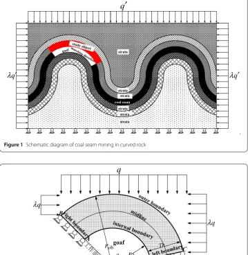
According to the shape and stress ﬁeld characteristics of the curved strata, a schematic diagram of coal seam mining in the curved strata is set up as shown in Fig.1. Here, the shape of the curved rock is simpliﬁed to a circular arc shape. The research object in this section is the overlying strata in the goaf, which is marked in red in Fig.1.

6.1 Numerical calculation model

Figure2is a plane strain model for numerical calculation of curved strata. When the dis-placement function method is used to solve the computational model, the nodes in the computational domain should satisfy the governing equation for displacement function, and the boundary conditions should satisfy the boundary conditions as shown in Table1. Special care has been taken to model the boundary conditions at the four corner nodes,

.

Figure 1Schematic diagram of coal seam mining in curved rock

(14)

Table 1 Boundary conditions of the computational model

Boundary Boundary conditions

Normal component Tangential component Right Boundaryθ=θi ur(r,θi) = 0 uθ(r,θi) = 0

Left Boundaryθ=θmax=θi+θe ur(r,θmax) = 0 uθ(r,θmax) = 0

Inner Boundaryr=rib σr(rib,θ) = 0 τrθ(rib,θ) = 0

Out Boundaryr=rob,θ≤90◦ σr(rob,θ) = –q(λcosθ+ sinθ) τrθ(rob,θ) = –q(cosθ–λsinθ)

Out Boundaryr=rob,θ> 90◦ σr(rob,θ) = –q(–λcosθ+ sinθ) τrθ(rob,θ) = –q(cosθ+λsinθ)

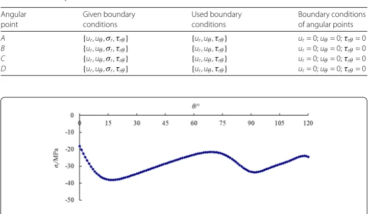
Table 2 Boundary conditions at four corners

Angular point

Given boundary conditions

Used boundary conditions

Boundary conditions of angular points

A _{ur,uθ,σr,τrθ} {ur,uθ,τrθ} ur= 0;uθ= 0;τrθ= 0

B _{ur,uθ,σr,τrθ} {ur,uθ,τrθ} ur= 0;uθ= 0;τrθ= 0

C {ur,uθ,σr,τrθ} {ur,uθ,τrθ} ur= 0;uθ= 0;τrθ= 0

D {ur,uθ,σr,τrθ} {ur,uθ,τrθ} ur= 0;uθ= 0;τrθ= 0

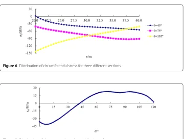
Figure 3Distribution of radial stress along the middle circumference

the details of which are illustrated in Table2. It can be seen from Table2that three out of the available four boundary conditions are satisﬁed at each corner nodes of the domain, and the remaining one is considered as redundant. It can be mentioned that usual com-putational approaches use two out of four conditions at each corner nodes to obtain the solution and thus the stresses around the corner regions deviate more from the actual stress state. Here, the mesh lengthhis 0.5 m and the mesh lengthkis 1◦.

6.2 Stress analysis of curved strata

Taking inner radiusrib= 20 m, the coeﬃcient of tectonic stressλ= 1.8, mining depthmd=

1000 m, advancing angleθe= 120◦, mining locationθi= 0◦, and rock thicknessst= 20 m

as examples, the distribution characteristics of radial stress in the computational model are given as follows.

6.2.1 Distribution of radial stress in curved strata

(15)

Figure 4Distribution of radial stress for three diﬀerent sections

Figure 5Distribution c of circumferential stress along the middle circumference

aroundθ= 15◦. It can be seen that the radial stress will reach a peak value not far from open-off cut. The distribution of radial stress for three different sections (θ= 45◦, 75◦and 105◦) is shown in Fig.4. The radial stress increases gradually from the inner surface to the outer surface along the radial direction, and the radial stress forθ = 45◦ increases faster comparing with the other two sections, which indicates that the radial stress increases faster for the section closer to open-off cut. On the contrary, the radial stress increases slow and the value of radial stress is small. It is worth mentioning that the radial stress values for all sections on the inner surface are zero, which indicate that the results conform to the boundary conditions of radial stress on the inner surface.

6.2.2 Distribution of circumferential stress in curved rock strata

(16)

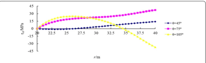
Figure 6Distribution of circumferential stress for three diﬀerent sections

Figure 7Distribution of shear stress along the middle circumference

forθ= 75◦is 40.99 MPa on the inner surface, while the value is 91.28 MPa on the outer surface. The circumferential stress forθ = 105◦decreases by about 70% from the inner surface to the outer surface. It should be mentioned that the value of circumferential stress for sections (θ= 75◦∼105◦) is larger than for other sections, which may easily cause the circumferential compression breaking in the overlying strata. Therefore, more observation should be carried out during the mining for these sections, and necessary measures should be taken for avoiding the disaster accidents.

6.2.3 Distribution of shear stress in curved strata

(17)

Figure 8Distribution of shear stress for three diﬀerent sections

7 Conclusions

In the present research, a modification to the usual approach of analyzing the plane curved beam with mixed boundary conditions in polar coordinates is introduced, which has been realized through the development of a displacement function based finite difference scheme. The novel of the present approach is that the governing equation for the plane problem is expressed in terms of a single partial differential equation. This method can handle mixed mode of boundary conditions, which is in contrast with the classical stress function formulation. Moreover, the finite difference scheme for governing equation, dis-placement components, and stress components has been developed, and the difference equations are also obtained in present paper. Finally, these theoretical formulations are applied to analyze the stress distribution of curved rock during the coal seam mining, which will provide scientific basis and reference for coal mining engineering.

Acknowledgements

The authors would like to thank the referees for careful reading and several constructive comments and for making some useful corrections that have improved the presentation of this paper.

Funding

Financial support for this work, provided by the National Fund for Nature projects (No. 51574228), the Research Foundation of Heze University (No. XY17KJ03) and Engagement Fund of Heze University (NO. XYPY02), the General Project of Science and Technology Plan of Shandong University (J17KB044), and General Items of Teaching Reform of Heze University (2016064), is gratefully acknowledged.

Availability of data and materials

This paper does not analyse or generate any datasets.

Competing interests

The authors declare that they have no competing interests.

Authors’ contributions

The authors have achieved equal contributions. All authors read and approved the manuscript.

Publisher’s Note

Springer Nature remains neutral with regard to jurisdictional claims in published maps and institutional aﬃliations.

Received: 16 November 2018 Accepted: 4 April 2019 References

1. Timoshenko, S.P., Goodier, J.N.: Theory of Elasticity. Mc Graw-Hill Book Company, New York (1979) 2. Zhi-lun, X.: Mechanics of Elasticity. Higher Education Press, BeiJing (2002)

3. Mcclay, K.R., Price, N.J.: Thrust and Neppe Tectonics, pp. 9–544. Geological Social, London (1981) 4. Mcclay, K.R.: Thrust Tectonics. Chapman & Hall, London (1992) 447

5. Ding, H., Shu, C.: A stencil adaptive algorithm for finite difference solution of incompressible viscous flows. J. Comput. Phys.214(1), 397–420 (2006)

(18)

7. Bieniasz, L.K.: Experiments with a local adaptive grid h-refinement for the finite-difference solution of BVPs in singularly perturbed second-order ODEs. Appl. Math. Comput.195(1), 196–219 (2008)

8. Hossain, M.Z., Ahmed, S.R., Uddin, M.W.: Generalized mathematical model for the solution of mixed-boundary-value elastic problems. Appl. Math. Comput.169(2), 1247–1275 (2005)

9. Xu, W., Li, G.: Finite diﬀerence three-dimensional solution of stresses in adhesively bonded composite tubular joint subjected to torsion. Int. J. Adhes. Adhes.30(4), 191–199 (2010)

10. Nath, S.K.D., Ahmed, S.R.: A displacement potential-based numerical solution for orthotropic composite panels under end moment and shear loading. J. Mech. Mater.4(6), 987–1004 (2009)

11. Mc Corquodale, P., Colella, P., Grote, D.P., Vay, J.L., et al.: A node-centered local reﬁnement algorithm for Poisson’s equation in complex geometries. J. Comput. Phys.201(1), 34–60 (2004)

12. Li, Z.L., Dou, L.M., Cai, W., et al.: Investigation and analysis of the rock burst mechanism induced within fault-pillars. Int. J. Rock Mech. Min. Sci.70, 192–200 (2014)

13. Chen, X.H., Li, W.Q., Yan, X.Y.: Analysis on rock burst danger when fully-mechanized caving coal face passed fault with deep mining. Saf. Sci.50, 645–648 (2012)

14. Jiang, Y.D., Wang, T., Zhao, Y.X., et al.: Experimental study on the mechanisms of fault reactivation and coal bumps induced by mining. J. Coal Sci. Eng.19, 507–513 (2013)

15. Ji, H.G., Ma, H.S., Wang, J.A., et al.: Mining disturbance eﬀect and mining arrangements analysis of near-fault mining in high tectonic stress region. Saf. Sci.50, 649–654 (2012)

16. Li, M., Zhang, J.X., Liu, Z., Zhao, X., Huang, P.: Mechanical analysis of roof stability under nonlinear compaction of solid backﬁll body. Int. J. Min. Sci. Technol.26(5), 863–868 (2016)

17. Li, Z.L., Dou, L.M., Cai, W., et al.: Investigation and analysis of the rock burst mechanism induced within fault-pillars. Int. J. Rock Mech. Min. Sci.70, 192–200 (2014)

18. Chen, X.H., Li, W.Q., Yan, X.Y.: Analysis on rock burst danger when fully-mechanized caving coal face passed fault with deep mining. Saf. Sci.50, 645–648 (2012)

19. Jiang, Y.D., Wang, T., Zhao, Y.X., et al.: Experimental study on the mechanisms of fault reactivation and coal bumps induced by mining. J. Coal. Sci. Eng.19, 507–513 (2013)

20. Cook, R.D.: Axisymmetric ﬁnite element analysis for pure moment loading of curved beams and pipe bends. Comput. Struct.33(2), 483–487 (1989)

21. Rattanawangcharoen, N., Bai, H., Shah, A.H.: A 3D cylindrical ﬁnite element model for thick curved beam stress analysis. Int. J. Numer. Methods Eng.59(4), 511–531 (2004)

22. Richards, T.H., Daniels, M.J.: Enhancing ﬁnite element surface stress predictions: a semi-analytic technique for axisymmetric solids. J. Strain Anal. Eng. Des.22(2), 75–86 (1987)

23. Smart, J.: On the determination of boundary stresses in ﬁnite elements. J. Strain Anal. Eng. Des.22(2), 87–96 (1987) 24. Gangan, P.: The curved beam/deep arch/ﬁnite ring element revisited. Int. J. Numer. Methods Eng.21(3), 389–407

(1985)

25. Dow, J.O., Jones, M.S., Harwood, S.A.: A new approach to boundary modeling for ﬁnite diﬀerence applications in solid mechanics. Int. J. Numer. Methods Eng.30(1), 99–113 (1990)

26. Ranzi, G., Gara, F., Leoni, G., Bradford, M.A.: Analysis of composite beams with partial shear interaction using available modeling techniques: a comparative study. Comput. Struct.84(13–14), 930–941 (2006)