Self optimization of coverage and capacity based on a fuzzy neural network with cooperative reinforcement learning

R E S E A R C H

Open Access

Self-optimization of coverage and capacity

based on a fuzzy neural network with

cooperative reinforcement learning

Shaoshuai Fan

, Hui Tian

and Cigdem Sengul

Abstract

Self-organization is a key concept in long-term evolution (LTE) systems to reduce capital and operational expenditures (CAPEX and OPEX). Self-optimization of coverage and capacity, which allows the system to periodically and

automatically adjust the key radio frequency (RF) parameters through intelligent algorithms, is one of the most important tasks in the context of self-organizing networks (SON). In this paper, we propose self-optimization of antenna tilt and power using a fuzzy neural network optimization based on reinforcement learning (RL-FNN). In our approach, a central control mechanism enables cooperation-based learning by allowing distributed SON entities to share their optimization experience, represented as the parameters of learning method. Specifically, SON entities use cooperative Q-learning and reinforced back-propagation method to acquire and adjust their optimization experience. To evaluate the coverage and capacity performance of RL-FNN, we analyze cell-edge performance and cell-center performance indicators jointly across neighboring cells and specifically consider the difference in load distribution in a given region. The simulation results show that RL-FNN performs significantly better than the best fixed configuration proposed in the literature. Furthermore, this is achieved with significantly lower energy consumption. Finally, since each self-optimization round completes in less than a minute, RL-FNN can meet the need of practical applications of self-optimization in a dynamic environment.

Keywords: LTE; Self-organizing network; Coverage and capacity; Fuzzy neural network; Reinforcement learning

1 Introduction

Today’s cellular radio technologies are developed to oper-ate closer to Shannon capacity bound. Yet, efficient PHY layer solutions may not necessarily translate to efficient resource utilization as the network performance relies on the dynamics of the radio network environment [1]. To this end, one of the key concepts of the prominent 4G technology, long-term evolution (LTE), is self-organizing network (SON), which is expected to help LTE cope with network and traffic dynamics both during deploy-ment and operation [2]. Essentially, SON, which enables self-configuration, self-optimization, and self-healing, is expected to improve network performance and user

*Correspondence: [email protected]

1State Key Laboratory of Networking and Switching Technology, Beijing University of Posts and Telecommunications, Beijing 100876, China Full list of author information is available at the end of the article

quality of experience while reducing capital expenditures (CAPEX) and operational expenditures (OPEX) [3-7].

Coverage and capacity optimization (CCO) is one of the typical operational tasks of SON [2,8]. CCO allows the system to periodically adjust to the changes in traffic (i.e., load and location) and the radio environment by adjust-ing the key radio frequency (RF) parameters (e.g., antenna configuration and power) through intelligent algorithms. For the online CCO problem, there is no definite mapping function from the inputs and parameters to be adjusted to the coverage and capacity performance. The main rea-son is the complexity of adjusting all the configuration parameters affecting both coverage and capacity. In addi-tion, the configuration parameter space is too large, which prohibits exhaustive search [9]. Thereby, most algorithms are designed in a heuristic way.

Among the existing approaches, the artificial intel-ligence-based approaches that accumulate the operational

and optimization experience and form optimization poli-cies based on these experiences are the most promis-ing. The optimization experience, which is shared among SON entities, constitutes traffic and radio conditions, and current configuration and performance. Current config-uration is typically defined based on a single optimiza-tion parameter (e.g., antenna tilt) and does not take into account the impact of other parameters such as power in optimizing capacity and coverage. Also, learning is typi-cally performed in a selfish manner without considering the learning cooperation of all the entities.

To overcome the aforementioned problems, in this paper, we design a distributed fuzzy neural network (FNN) to guide the joint optimization of coverage and capacity. Our solution introduces a central control mecha-nism to facilitate cooperative learning by sharing the opti-mization experience of SON entities. As the core part of the fuzzy neural network, both fuzzy inference rule base and parameters of membership functions are acquired and adapted with reinforcement learning method which can achieve a predefined goal by directly interacting with its uncertain environment and by properly utilizing past experience derived from previous actions. To control cov-erage and capacity, we jointly optimize antenna tilt and power while considering the varied and non-uniform traffic load distribution of the cells within a specific region.

The rest of the paper is organized as follows. In Section 2, we describe related research in the literature. In Section 3, we discuss the factors that affect our approach and describe the architecture for CCO. In Section 4, we present the details of the proposed reinforcement learning-based FNN optimization (RL-FNN) executed in distributed SON entities. In Section 5, we present the simulation results. Finally, we draw the conclusions in Section 6.

2 Related work

Majority of the coverage and capacity optimization algorithms are heuristic due the complexity of the prob-lem. For instance, local search methods, such as gra-dient ascent [10] and simulated annealing [11,12], are adopted for radio network planning. In [10], a heuris-tic variant of the gradient ascent method was adopted to optimize antenna tilt. In [11,12], simulated annealing algo-rithm was used to control the downlink transmit power. The proposed approaches rely on the accurate down-link interference information in an eNodeb’s own and neighboring cells under all possible parameter configura-tions. However, such information can hardly be predicted due to not having a precise mapping from parameter adjustments to the current performance. Taguchi method, which is superior to the local search methods in explor-ing the search space, was used in [13] to optimize

radio network parameters. Yet, a great number of exper-iments are needed to explore the large parameter space and determine the impact of different parameter values on the network performance during operation. Finally, in all these algorithms, each iteration step caused by the dynamics in traffic and the radio environment is a trial-and-error process. Due to the risk of negative per-formance impact, trial-and-error is prohibitive in real networks.

To prevent potential drastic changes in the network performance, the artificial intelligence approach, which can accumulate the operational and optimization expe-rience and form optimization policies based on the experience, has significant potential [14-17]. In [1,18], a case-based reasoning algorithm enables distributed decision-making. The algorithm stores past successful optimization instances that improved the performance in the memory and applies these instances directly to new situations. In [19-21], a fuzzy Q-learning algorithm was used to learn the optimal antenna tilt control policy based on the continuous inputs of current antenna con-figuration and corresponding performance, and output of the optimized antenna configuration. Yet, the impact on neighboring cells due to such an adjustment was neglected. To overcome the suboptimal performance of selfish learning, the approaches proposed in [6,22] per-mit the cells to share their performance statistics with their neighbor cells so that each SON entity tries to learn the optimal action policy based on the overall reward of the neighborhood instead of local selfish rewards. However, the potential from having SON entities learn cooperatively was not taken into consideration. Also, the fuzzy membership functions in the proposed fuzzy Q-learning algorithms were predefined by intuition or partial operation experience, which may affect the opti-mization performance. Moreover, in contrast to our approach, these approaches only optimize the antenna tilt.

3 Coverage and capacity optimization under

hybrid SON architecture

To achieve capacity and coverage optimization (CCO), we adopt the hybrid architecture shown in Figure 1. On one hand, each site has SON entities corresponding to each sector (three sectors in our study), and each entity runs its optimization process in a distributed manner which can provide fast adaptation. On the other hand, a central entity located in the network management system (NMS) is needed whose main function, in our proposed approach, is to realize the cooperation of distributed optimization by collecting optimization experience of all distributed entities and sharing them in a global manner.

Figure 1Hybrid SON architecture for CCO.

adjusting the RF parameters which affect downlink signal to interference plus noise ratio (SINR):

SINRij=

where Pi is the transmit power on each resource block (RB) which is in direct proportion to the total power of eNodeB i if the power is equally allocated, N is the received noise, and Gij is the link loss from eNodeB i to user j including path loss, antenna gain, shadowing, multipath fading, etc.

Antenna configuration and total power are the key RF parameters for optimization. For 3D antenna con-figuration, there are four important parameters that can be adjusted: antenna azimuthϕas, horizontal half-power beam width ϕ3dB, vertical half-power beam width θ3dB, and remote electrical tilt (RET)θgtilt. The antenna config-uration parameters affect the three-dimensional antenna gainA(ϕ,θ )as follows [23]:

A(ϕ,θ )= −min{−[AH(ϕ)+AV(θ )] ,Am}. (2) The horizontal antenna gain and vertical antenna gain are defined as

In Equations 3 and 4,Amdenotes the maximum antenna front-to-back attenuation and SLAv denotes the maxi-mum vertical slant angle attenuation.

While the RET optimization can provide larger gains in terms of cell-edge and cell-center performance [1], power optimization can improve coverage and capacity

performance and also power efficiency to some extent. Considering these factors, the antenna tilt and total power are chosen as the parameters to adjust in order to improve the coverage and capacity performance.

Many factors should be considered while adjusting the RF parameters, including edge performance, cell-center performance, inter-cell interference, and traffic load distribution. For instance, a higher value of antenna tilt or a lower value of power may result in coverage out-age at the cell-edge but will also result in less inter-cell interference. On the contrary, a lower antenna tilt or a higher power may result in expansion of coverage and improvement of cell-edge performance with the risk of more inter-cell interference. Additionally, the expanded coverage of a cell may relieve the traffic load in neighbor-ing cells at the risk of causneighbor-ing congestion in the expanded cell. Consequently, the fact that all the adjustments have both negative and positive consequences makes this opti-mization problem very complex to solve.

However, note that regardless of the underlying rea-son, all adjustments will affect the throughput of users. Therefore, we adopt throughput as the metric for evalu-ating system performance. Obviously, there is a trade-off between coverage and capacity. Typically, more coverage results in less capacity due to deteriorating signal power, and one cannot optimize both coverage and capacity at the same time. To achieve a trade-off, we define the key performance indicator (KPI) of an optimization area, e.g., sectori, as

KPIi=ωTi5%+(1−ω)Ti50%. (5)

In Equation 5,Ti5% represents cell-edge coverage, which

is computed as the throughput cumulative distribution function (CDF) of 5% tile, and Ti50% denotes the

cell-center capacity, computed as the throughput CDF of 50% tile. Also, a weight factorωis used to balance coverage and capacity performance. In this paper, we give more weight to the coverage performance as it affects user experience more.

The adjusting of the RF parameters will also have an impact on neighboring regions. Hence, the KPI of the neighbor regions should also be taken into account dur-ing the optimization. Then, the coverage and capacity optimization problem can be formulated as a joint KPI maximization problem for a regioni:

max

of the optimization ability. Note that the setting of these weights depends on the network operators’ optimization targets and strategies. Finally, as each SON entity solves the CCO problem locally, we assume that the KPI infor-mation, needed from the neighboring cells, can be easily transferred via LTE X2 interfaces between eNodeBs.

4 Fuzzy neural network with cooperative

Q-learning

In this paper, our main goal is to enable all SON enti-ties to take simultaneous actions periodically to optimize RF parameters and learn from each other’s optimization experience. In order to achieve this, we propose using a distributed Q-learning based fuzzy neural network algo-rithm, which we present in detail in this section.

4.1 Architecture of RL-FNN

The proposed RL-FNN is similar in architecture to [24,25] and consists of five layers. Figure 2 shows each layer, where layer 1 consists of the input nodes, layer 2 consists of the rule antecedent nodes, layer 3 consists of the rule nodes, layer 4 consists of the rule consequent nodes, and layer 5 consists of the output nodes.

The proposed RL-FNN has two generic processes: for-ward operation and learning. It describes the current state based on the current power and tilt configuration, and the corresponding coverage and capacity performance are taken into account in every forward operation process to obtain the best RF parameters. RL-FNN performs the mapping function of current state to the best RF con-figuration in the forward operation process, while the mapping function is formed by the learning process. How-ever, considering that the perfect input-output training sample pairs can hardly be acquired in a realistic network, reinforcement learning methods [26,27] are needed for training the fuzzy neural network.

Figure 2Architecture of RL-FNN.

In addition, we have to keep in mind that in certain applications, the performance of fuzzy neural network highly depends on the fuzzy inference rule base and the particular membership functions, which can strongly affect the performance. Therefore, RL-FNN adopts a two-phase learning process: knowledge acquisition and parameter learning. In the knowledge acquisition phase, cooperative Q-learning method is adopted to acquire the fuzzy inference rule base. In the parameter learning phase, we adopt the reinforced back-propagation method to adjust the parameters of fuzzy membership functions. The details of the forward operation process and the two-phase learning process are explained in the rest of this section.

4.2 Forward operation 4.2.1 Layer 1

In layer 1, the input of the RL-FNN is the current RF con-figuration and the corresponding performance. The RF configuration is described by the current power P and tilt θ, and the current performance is described by JKPI (see Equation 6). Note that JKPI is not only affected by the spectrum efficiency which is determined by the RF configuration, but also affected by the load distribution (e.g., the higher the traffic load, the lower the average allo-cated bandwidth and throughput of users). Therefore, we adopt two parameters to describe the current state: (1) the traffic load gap L, which reflects the variation of load distribution among neighboring cells, and (2) the spec-trum efficiency indicator gapS, which reflects variation in coverage and capacity performance without the effect of the traffic load. More specifically, L represents the normalized difference between traffic loadLof the sector and the average loadL¯of its neighboring sectors:

L= L− ¯_¯ L

L . (7)

Srepresents the normalized difference between cover-age and capacity performance indicatorSof the sector and the average performanceS¯of its neighboring sectors:

S= S− ¯_¯ S

S . (8)

Similar to the definition of KPI,S=ωS5%+(1−ω)S50%,

whereS5%denotes the spectrum efficiency CDF of 5% tile

andS50%denotes the spectrum efficiency CDF of 50% tile.

corresponding to four input variables. The inputI_i(1)and outputO(_i1)of nodeN_i(1)in layer 1 are defined as

O(_i1)=I_i(1)=xi. (9) 4.2.2 Layer 2

In this layer, each input variable is fuzzified into three lin-guistic levels - high (H), medium (M), and low (L) - which are also called Gaussian fuzzy sets. So, this layer consists of 12 nodes. Each rule antecedent node N_ij(2) calculates the degree of membership for thejth Gaussian fuzzy set associated with theith input variable. The inputI_ij(2)and outputO(_ij2)of nodeN_ij(2)in layer 2 are defined as dard deviation of the Gaussian membership function of layer 2.

4.2.3 Layer 3

Each rule node N_k(3) in this layer represents a possible IF part of an IF-THEN fuzzy inference rule and function to compute the overall degree of similarity between the observed inputs and the antecedent conditions of thekth fuzzy inference rule. This layer consists of 81 nodes cor-responding to 81 possible combinations of the linguistic inputs. The inputI_k(3)and outputO_k(3)of nodeN_k(3)in layer 3 are defined as

I_k(3)=(O(₁2_k)

i is the degree of membership of theith linguistic input for the IF part of thekth fuzzy inference rule.

4.2.4 Layer 4

Each of the two output variables of RL-FNN is fuzzified into three linguistic levels - high (H), medium (M), and low (L). So, this layer consists of six nodes. The links from layer 3 nodes to layer 4 nodes denote the THEN part of the IF-THEN fuzzy inference rules. The method of estab-lishing the fuzzy inference rule base will be described in Section 4.3.

The rule consequent node N_lm(4) in layer 4 performs consequent derivation using the set of IF-THEN fuzzy inference rules. Each rule consequent node sums the out-put of the layer 3 nodes, which see this layer 4 node as a consequence, to identify the degree of membership for the

consequent part of the rule. The inputI_lm(4)and outputO(_lm4) Gaussian fuzzy set associated with thelth output variable.

4.2.5 Layer 5

The best configuration value of powerP and tiltθ for current state is obtained in this layer as the outputs of RL-FNN. This layer consists of two output nodes correspond-ing to two output variables (P,θ). The output nodes finally perform defuzzification of the overall inferred out-put fuzzy set according to the center of area method. The input I_l(5) and output O_l(5) of node N_l(5) in layer 5 are dard deviation of the Gaussian membership function of layer 5. The method of acquiring the Gaussian member-ship function parameters of layer 2 and layer 5 will be described in Section 4.4.

4.3 Q-learning for knowledge acquisition

In order to achieve self-optimization, each entity in each cell must know what parameter tuning action should be done according to the current operation state which is determined byx=(P,θ,L,S)(defined in Section 4.2). However, it is hard to populate the fuzzy inference rule base, as the complete and accurate knowledge of the network operation can hardly be acquired online, and typically, not enough operational experience can be col-lected beforehand in such a complex optimization sce-nario. Therefore, in our approach, cooperative Q-learning algorithm is used for knowledge acquisition.

For each rule, there are nine possible inference results corresponding to the combinations of the linguistic out-puts. The possible results of kth rule in Q-learning are shown as

IF current state is the antecedent state of thekth rule THENPis high and θis high withq_k1,

or Pis high and θis medium withq_k2,

· · · ·

Here qki represents the elementary quality of the ith inference result responding to kth rule, and the higher value of q_ki, the higher the trust for the corresponding power and antenna setting.

The action of the kth rule is chosen by an explo-ration/exploitation policy using ε-greed method as fol-lows:

Here, the greed action factorεis decreased to zero as the optimization step increases.

The best fuzzy inference rules are obtained by using the quality functionQπ(s,a) that is defined as the expected sum of discounted rewards from the initial states0under

policyπas follows:

Qπ(s,a)=Eπ[ ∞

t=0

γtr(st,at)|s0=s,a0=a] . (19)

In Equation 19,standat denote the state and the action of the fuzzy inference rule at stept, andγ is the discount factor.

The Q-learning algorithm solves the quality function iteratively using the following temporal difference update:

Qt+1(st,at)=Qt(st,at)+Qt. (20) To define the incremental quality of quality functionQ, the reward value, the quality function, and the value func-tion are needed. The reward value is defined as the JKPI difference between recent learning steps:

rt=JKPI=JKPIt+1−JKPIt. (21) The quality function of the activated rules is calculated as

Qt(st,at)=

k

O(_k3)qkc(k). (22) The value function of the new state after performing the applied action is calculated as:

Vt(st+1)=

k

O(_k3)max

i qki. (23)

So, using the above three parameters,Qis calculated as

Qt=ξ(rt+1+γVt(st+1)−Qt(st,at)) (24) and the elementary qualityq_kishould be updated by

qki= ξO (3)

k Q, ifi=c(k)

0, otherwise . (25)

In Equation 25,ξis the learning rate for Q-learning. All distributed self-optimization entities perform the same learning function in similar conditions. So, the learning experience of any distributed entity, which is represented as the parameters of learning method, can

be used by another entity. Enabling cooperative learn-ing through sharlearn-ing quality values can also improve the learning speed and the quality of the fuzzy inference rule base. To share their experience, after every learning step of Q-learning, each entity updates its quality values of the rules according to the overall shared experience. To counter for the fact that different entities may have dif-ferent experiences under similar dynamics, we use the average experience over all entities and calculate it as

qj_ki= 1

Here, qj_ki denotes the quality value recorded in self-optimization entity j corresponding to the ith action of

the kth rule, and M is the number of the SON

enti-ties managed by the central network management system (NMS).

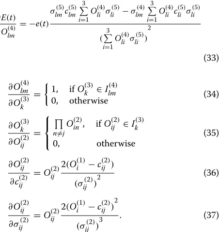
4.4 Reinforced parameter learning

The reinforcement learning procedure [27] is executed to enable error back-propagation that minimizes a quadratic error function. Specifically, a reinforcement signal is prop-agated from the top to the bottom of the five-layered fuzzy neural network. Here, the parameters to adapt are the means and standard deviations of the fuzzification and defuzzification Gaussian membership. The quadratic error function is defined as

E(t)= 1

2e

2_(t)= 1

2(y

∗_−y(t))2_{, (27)}

where y∗ denotes the best overall experienced value of the JKPI, y(t) denotes the measured JKPI at step t, and

e(t) = y∗−y(t)denotes the reinforcement signal. Con-sequently, as a result of the reinforcement learning, the algorithm adapts parameters of RL-FNN to minimizeE(t), which is equivalent to maintaining the overall JKPI at the best experienced value.

To update a parameterZ(t), we calculate

Z(t+1)=Z(t)−η∂E

∂Z. (28)

σ_lm(5)(t+1)=σ_lm(5)(t)

Similarly, the corrections of the mean and standard deviation of the fuzzification Gaussian membership func-tion are calculated as

c(2)_ij (t+1)=c(2)_ij (t)−η

The transmissions of reinforcement signal in each layer are as follows:

Similar to the quality values in Section 4.3, the SON entities also share their learning experience of RL-FNN membership function parameters. Again, after each learn-ing step, each distributed entity updates the mean and standard deviation parameters according to the overall experience. The sharing of parameters can be represented as

Here, Zj denotes the vector of the mean and stan-dard deviation parameters recorded in self-optimization entityj.

5 Simulation and analysis

The proposed approach is evaluated by system level LTE networks simulator developed in c++. The simulation parameters and placement of transceivers (TRs) are set based on the interference-limited scenario with a hexago-nal macro-cell deployment described in [23,28]. We sim-ulate 7 three-sector cells with an inter-site distance of 500 m. Twenty to sixty users are uniformly distributed in each cell, maintaining 35 m minimum distance to the base station. The user mobility is modeled with random walk with a constant speed of 3 km/h (wrapping around is permitted). Users always have a full buffer (i.e., they have always traffic to send), and we use round robin scheduling. The additional details of our network configuration and RL-FNN parameter settings are listed in Table 1.

For comparison, we define a reference RF configuration where all cells have the same fixed antenna tilt of 15◦and fixed total power of 46 dBm. This configuration was found to be the best configuration using discrete exhaustive search method for our simulated scenario [22,23].

5.1 Details on operation of RL-FNN

In this section, we present the details of the RL-FNN algorithm and how it computes the degrees of fuzzy membership functions and does the inference for our simulation scenario.

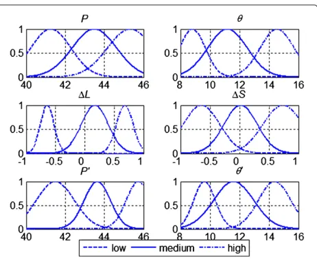
As an example, Figure 3 shows the fuzzy membership functions acquired by reinforcement learning at optimiza-tion step 1,200 in our simulaoptimiza-tion process.

The membership functions determine which fuzzy set the input value belongs to and the degree of the member-ship. The shapes of the Gaussian membership functions determined by the optimized means and standard devi-ations will help to determine these factors in a more accurate way to improve the performance of the fuzzy neural network.

Table 1 Simulation parameters

Parameter Value

Carrier frequency 2.0 GHz

Channel bandwidth 10 MHz

Propagation loss ₋128.1₋37.6 log10(d),din km

Shadowing standard deviation 8 dB

Shadowing correlation distance 50 m

Shadowing correlation Intersite, 0.5; intersector, 1.0

Penetration loss 20 dB

Thermal noise density −174 dBm/Hz

BS maximum transmit power 46 dBm

Maximum antenna front-to-back attenuationAm

25 dB

Maximum vertical slant angle attenuation SLAv

20 dB

Horizontal half-power beam width ϕ3dB

70◦

Vertical half-power beam width θ3dB

10◦

BS and UE antenna height 32 m; 1.5 m Power allocation on channels Equal allocation

Self-optimization time 100 ms interval(learning time interval)

KPI weight factorω 0.8

JKPI weight factorα 0.5

Initial greed action factorε 0.1 Reducing rate of greed action 0.001/s factor

Discount factorγ 0.7

Learning rate for Q-learningξ 0.5 Parameter learning factorη 0.2

to less inference to neighbors, more antenna gain to users in the current cell and load redistribution. However, it cannot be known which of these factors cause the highest improvement and some even may cause negative effects, but nevertheless the overall performance will improve.

5.2 Evaluation of coverage and capacity

In order to test the CCO performance of RL-FNN, we start the simulation with a poor configuration with very low power and very low antenna tilt, which are 8◦and 40 dBm, respectively. After the initialization, RL-FNN approach starts to be executed in all entities periodically to optimize the coverage and capacity performance.

Figure 4 shows the initial and the resulting SINR dis-tributions excluding shadow fading. In Figure 4a, due to the poor initial configuration, SINR value is lower than 10 dB in almost the entire area which results in poor net-work coverage and capacity performance. As the entities

Figure 3Membership functions acquired by reinforcement learning.

in cells learn the optimization experience cooperatively and optimize their RF configurations periodically, the SINR situation improves to be greater than 15 dB (see Figure 4b).

The average JKPI of overall sectors during the opti-mization process is shown in Figure 5. Initially, JKPI is very low and with RL-FNN improves from approximately 175 to 200 kbps at the very beginning of the optimiza-tion. The reason for this fast improvement is that at the beginning, entities without any experience will ran-domly choose the fuzzy inference rules. This extends the range of configuration adjustment and avoids being lim-ited to a local configuration space. Later, entities gradually learn and share the operation experience of which learn-ing parameters and RF configurations may result in a better performance. In addition, the entities still execute exploration policy according to Equation 18, which allows accumulating a diverse set of experiences. However, the side effect of such explorations is the resulting tempo-rary low JKPI. Figure 5 shows that, generally, RL-FNN gradually improves the JKPI. After about step 700, 70 s after the initialization, we do not see significant improve-ment in JKPI, and JKPI converges to around 220 kbps although it still fluctuates slightly due to the mobility of users and dynamics of channel conditions. In addition, the JKPI is higher than that achieved by the reference which is regarded as the best configuration and was not out-performed in [21,22]. The improvement of JKPI comes from optimizing RF configurations according to the local traffic load distribution, which improves the resource uti-lization while the reference configuration cannot adapt to the traffic dynamics.

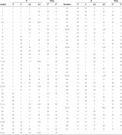
Table 2 Fuzzy inference rule base acquired by Q-learning

If Then If Then

Number P θ L S P θ Number P θ L S P θ

1 L L L L L H 43 M M H L L L

2 L L L M M H 44 M M H M H L

3 L L L H L L 45 M M H H M L

4 L L M L M H 46 M H L L H H

5,6 L L M M,H L H 47 M H L M M H

7 L L H L H H 48 M H L H L H

8 L L M H M H 49,50 M H M L,M L L

9 L L H H M L 51 M H M H H L

10 L M L L H H 52 M H H L L H

11 L M L M M H 53 M H H M M H

12 L M L H M L 54 M H H H M M

13 L M M L L M 55,56 H L L L,M L M

14 L M M M M H 57 H L L H L L

15 L M M H M M 58 H L M L H M

16 L M H L L H 59 H L M M M M

17,18 L M H M,H L M 60 H L M H L M

19 L H L L M H 61 H L H L L M

20 L H L M L H 62 H L H M H L

21 L H L H L M 63 H L H H M M

22 L H M L M H 64,65 H M L L,M L M

23 L H M M M M 66 H M L H H M

24 L H M H M H 67 H M M L M H

25,26 L H H L,M H M 68 H M M M M M

27 L H H H L L 69 H M M H H H

28 M L L L M M 70 H M H L L H

29 M L L M H L 71 H M H M L M

30 M L L H L L 72 H M H H M M

31,32 M L M L,M M M 73 H H L L H M

33 M L M H M L 74,75 H H L M,H M M

34 M L H L M H 76 H H M L L L

35 M L H M M M 77 H H M M M H

36 M L H H H M 78 H H M H H L

37,38 M M L L,M L H 79 H H H L L H

39 M M L H L H 80 H H H M L M

40 M M M L H M 81 H H H H H L

41,42 M M M M,H L M

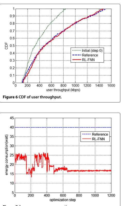
the coverage (i.e., 5% tile of user throughput) and capacity (i.e., 50% tile of user throughput) performance of RL-FNN are improved by 19.5% and 48.9%. Compared to the reference configuration, the coverage and capacity per-formance are also improved by 7.9% and 1.5%. However, from the CDF figure, we can also see that the reference is able to achieve higher throughput values and RL-FNN

Figure 4Simulated network SINR distribution excluding shadow fading.(a)To be optimized (step 0).(b)Optimized (step 1,200).

5.3 Additional benefits: energy efficiency

Adapting total power may also improve overall energy efficiency in addition to coverage and capacity. Figures 7 and 8 show the average energy consumption and the aver-age energy efficiency, respectively, during optimization process. We compute energy efficiency as throughput per watt. It is evident that the energy consumption of RL-FNN is much lower and the energy efficiency is much higher than the reference.

Figure 5Average JKPI.

Figure 6CDF of user throughput.

Figure 7Average energy consumption.

Table 3 Performance comparison

Indicator RL-FNN Reference Improvement

(%)

JKPI 219.6 kbps 209.2 kbps 5.0

Energy consumption 42.3 dBm (16.8 W) 46 dBm (39.8 W) 57.8

Energy efficiency 13.1 kbps/W 5.26 kbps/W 147.1

The average JKPI, energy consumption, and energy effi-ciency comparison of RL-FNN and the reference after step 700 are listed in Table 3. RL-FNN can improve coverage and capacity by 5% compared to the best configuration found with exhaustive search but improves energy con-sumption by 57.8%, and energy efficiency improves by 147.1%. The huge improvement comes from the opti-mized RF configuration. On one hand, lower interference will be caused by cell-edge users of neighboring cells resulting from lower power. On the other hand, the cov-erage of cells is optimized considering the traffic distri-bution, and the antenna beam orientation is optimized to mainly serve UE traffic within the coverage area while minimizing the interference to other cells. Although the power is lower than the maximum setting, it is better utilized with the help of the optimized directed antenna beam.

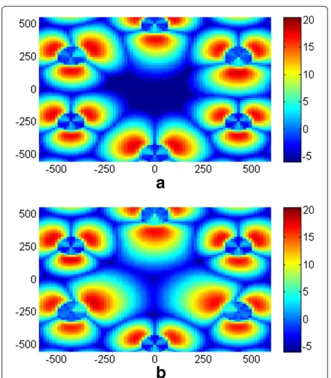
Figure 9Simulated network SINR distribution excluding shadow fading under abrupt changes.(a)To be optimized (step 1,201).(b) Optimized (step 2,400).

Figure 10Average JKPI under abrupt changes.

The above simulation results demonstrate that the pro-posed RL-FNN approach is able to achieve high perfor-mance in terms of coverage and capacity with significantly lower energy consumption.

5.4 Performance under abrupt changes

In this section, we evaluate the performance of RL-FNN when a cell is shut down due to, for instance, an unex-pected failure or for simply energy-saving purposes. In the simulation, a cell is shut down at the following step 1,201 and all entities execute RL-FNN approach periodically to optimize the coverage and capacity performance.

Figure 9 shows the SINR distribution comparison of the initial environment at step 1,201 and the optimized. When a cell is shut down, a coverage hole with a SINR of lower than−8 dB occurs which needs to be covered by the neighboring cells. This will consequently affect the

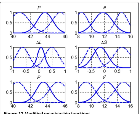
Figure 12Modified membership functions.

traffic load distribution of the neighboring cells. After the RF configurations are optimized, the hole is covered by neighboring cells with lower antenna tilts and the average SINR value in that area improves to 6.71 dB.

The variations of average JKPI of sectors nearby the coverage hole during optimization process after shutting down one cell are presented in Figure 10. At step 1,201, some of the users of the shut-down cell will be located in the coverage hole area and hence become the cell-edge users for the neighboring cells. This consequently wors-ens the cell-edge performance of those cells. So, the JKPI resulting from the RF configurations at step 1,201 is low but still higher than the reference due to the optimized

RF configurations in the previous optimization process. Later, the RL-FNN gradually improves the JKPI by adapt-ing the RF configurations to the new situation. At about step 1,700, 50 s after shutting down the cell, coopera-tive learning process converges with JKPI approximately around 170 kbps. There is no significant improvement after step 1,700.

Figure 11 shows the throughput CDF of the users in the coverage hole area and in the sectors nearby the coverage hole. Compared to performance at step 1,201, the cover-age and capacity performance of RL-FNN are improved by 33.4% and 7.0%, respectively. Compared to the reference configuration, the coverage and capacity performance are improved by 53.2% and 21.3%, respectively, achieving sig-nificant improvements.

The adapted fuzzy membership functions and fuzzy inference rules in the coverage hole scenario at step 2,400 are shown in Figure 12 and Table 4. There is a little dif-ference between the optimized shapes of the membership functions and those at step 1,200. The modifications of the membership functions are adapted to the coverage hole scenario and will help to determine the degree of member-ship function in a better way to improve the performance. Also, some of the fuzzy inference rules are modified. Compared to the old rules, we can see that entities become more likely to provide more power with lower antenna tilt to respond to the coverage hole. Take rule number 34 for example, when the power is medium, antennae tilt is low, traffic load compared to neighbors is high, and per-formance compared to neighbors is low, the best tuning action is to make the power higher while keeping low antenna tilt. That is to say, if a sector covers some users

Table 4 Modified fuzzy inference rules

If Then

Number P θ L S P θ

14,15 L M M M,H H L

18 L M H H M M

20,21 L H L M,H H H

23,24 L H M M,H L M

34 M L H L H M

35 M L H M H M

39 M M L H M H

42 M M M H H M

43 M M H L H M

45 M M H H M H

50 M H M M H L

69 H M M H M H

70,71,72 H M H L,M,H H L

Figure 13Average energy consumption under abrupt changes.

within the hole which will increase the traffic load and lower the performance, it is better for this sector to make the power higher in improving the performance. Conse-quently, potentially, more users within the hole can be covered by this sector. Another example is rule number 39: when the power is medium, antennae tilt is medium, traf-fic load compared to neighbors is low, and performance compared to neighbors is high, the best tuning action is to make the antenna tilt higher. This rule will mainly apply to the sector which is nearby the hole but cannot cover many users within the hole due to its antenna beam orientation. So it is better for this sector to make the antenna tilt higher which will lower the interference to users within the hole. In summary, different rules are acquired for different sit-uations, and the acquired rule base helps to improve the overall performance in the dynamic environment.

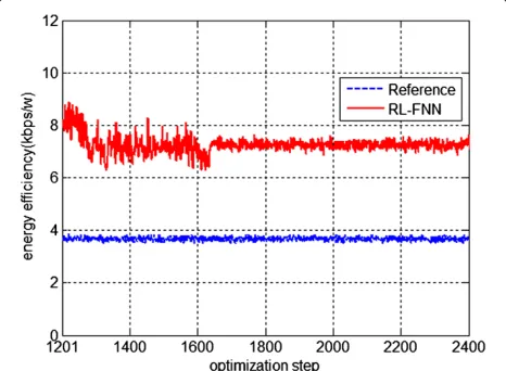
Figure 14Average energy efficiency under abrupt changes.

Table 5 Performance comparison under abrupt changes

Indicator RL-FNN Reference Improvement

(%)

JKPI 169.5 kbps 126.8 kbps 33.7

Energy consumption 43.7 dBm (23.2 W) 46 dBm (39.8 W) 41.7

Energy efficiency 7.3 kbps/W 3.2 kbps/W 128.1

Additionally, Figures 13 and 14, respectively, show the average energy consumption and the average energy effi-ciency during optimization process. It is evident that the energy consumption of RL-FNN is still lower and the energy efficiency is much higher than the reference in such a coverage hole scenario.

The average JKPI, energy consumption, and energy effi-ciency comparison of RL-FNN and the reference after step 1,700 are listed in Table 5. RL-FNN significantly improves coverage and capacity by 33.7%. Energy consumption is again low, with an improvement of 41.7% and energy effi-ciency improves 128.1%. Note that in this scenario, some of the neighboring cells lower their antenna tilts to cover the users located in the coverage hole. Therefore, more power than the initial step will be used due to these adaptations. Still the power is lower than the maximum constraint and is better utilized.

In summary, the simulation results demonstrate that the proposed RL-FNN approach can efficiently improve the coverage and capacity performance in a dynamic envi-ronment. The results show that in approximately 700 to 800 optimization steps, RL-FNN converges to a better setting than the reference from an initially badly chosen configuration. Also, in 500 to 600 steps, RL-FNN recov-ers from the coverage hole scenario. However, note that the actual time for reaching these states is determined by the time interval for the cell to collect the load and spectrum efficiency indicator of neighbors and to perform the adjustments. Given these considerations, we assume that the optimization step interval is approximately 0.1 s as our approach can operate with low granularity. Hence, we expect that RL-FNN can operate with convergence times in the order of a minute. Compared to [9,21,22] which need nearly 1,000 optimization steps for the one-dimensional optimization of antenna tilt, the convergence rate of RL-FNN is a significant improvement as it adjusts both power and antenna tilt. Such fast convergence rate can only be achieved by cooperative learning enabled by RL-FNN.

6 Conclusions

operate in a distributed manner and try to optimize power and antenna tilt automatically and cooperatively using the shared optimization experience.

From the simulation results, we conclude that our approach is able to acquire robust optimization poli-cies for different complex scenarios and maintains a sig-nificantly better performance in terms of coverage and capacity with low energy consumption. This especially results in a dramatic improvement in energy efficiency. Finally, RL-FNN converges with an acceptable rate and is therefore applicable to different dynamic scenarios and applications.

In our future work, variants of the algorithms will be developed to enhance the cooperation between SON enti-ties especially when abrupt changes happen. Moreover, it would be an interesting future research to extend the current work to heterogeneous networks.

Competing interests

The authors declare that they have no competing interests.

Acknowledgements

This work was supported by the National Natural Science Foundation of China (No. 61231009), National Major Science and Technology Special Project of China (No. 2013ZX03003016), National High Technology Research and Development Program of China (863 Program) (No. 2014AA01A705), and Funds for Creative Research Groups of China (No. 61121001).

Author details

1_{State Key Laboratory of Networking and Switching Technology, Beijing} University of Posts and Telecommunications, Beijing 100876, China. 2_{Department of Computing and Communication Technologies, Oxford} Brookes University, Wheatley, Oxford OX33 1HX, UK.

Received: 5 September 2013 Accepted: 3 April 2014 Published: 12 April 2014

References

1. ON ON Yilmaz, J Hämäläinen, S Hämäläinen, Optimization of adaptive antenna system parameters in self-organizing LTE networks. Wireless Netw.19(6), 1251–1267 (2013)

2. 4G Americas, White Paper: Self-optimizing networks: the benefits of SON in LTE (2013). http://www.4gamericas.org. Accessed on 7 October 3. SOCRATES: Self-optimisation and self-configuration in wireless networks.

http://www.fp7-socrates.eu.org. Accessed on 6–8 February 2008 4. 3GPP TS 32.500 Vb.1.0, Self-organizing networks (SON); Concepts and

requirements. http://www.3gpp.org. Accessed on 22 December 2011 5. 3GPP TR 36.902 V9.3.1, E-UTRA; Self-configuring and self-optimizing

network (SON) use cases and solutions. http://www.3gpp.org. Accessed on 7 April 2011

6. 3GPP TS 32.541 Vb.0.0: SON; Self-healing concepts and requirements. http://www.3gpp.org. Accessed on 7 April 2011

7. D Lopez-Perez, X Chu, AV Vasilakos, H Claussen, On distributed and coordinated resource allocation for interference mitigation in self-organizing LTE networks. IEEE/ACM Trans. Netw.21(4), 1145–1158 (2013)

8. S Sengupta, S Das, M Nasir, AV Vasilakos, W Pedrycz, An evolutionary multiobjective sleep-scheduling scheme for differentiated coverage in wireless sensor networks. Syst. Man Cybernet. Part C: Appl. Rev. IEEE Trans. 42(6), 1093–1102 (2012)

9. J Li, J Zeng, X Su, W Luo, J Wang, Self-optimization of coverage and capacity in LTE networks based on central control and decentralized fuzzy Q-learning. Int. J. Distributed Sensor Netw.2012(2012) 10. H Eckhardt, S Klein, M Gruber, Vertical antenna tilt optimization for LTE

base stations, inVehicular Technology Conference (VTC Spring) 2011 IEEE 73rd(Yokohama, May 2011), pp. 1–5

11. I Siomina, P Varbrand, D Yuan, Automated optimization of service coverage and base station antenna configuration in UMTS networks. Wireless Commun. IEEE.13(6), 16–25 (2006)

12. T Cai, GP Koudouridis, C Qvarfordt, J Johansson, P Legg, Coverage and capacity optimization in E-UTRAN based on central coordination and distributed Gibbs sampling, inVehicular Technology Conference (VTC 2010-Spring), 2010 IEEE 71st, Taipei(16–19, May 2010), pp. 1–5 13. A Awada, B Wegmann, I Viering, A Klein, Optimizing the radio network

parameters of the long term evolution system using Taguchi’s method. Vehicular Technol. IEEE Trans.60(8), 3825–3839 (2011)

14. Y Zeng, K Xiang, D Li, AV Vasilakos, Directional routing and scheduling for green vehicular delay tolerant networks. Wireless Netw.19(2), 161–173 (2013)

15. AV Vasilakos, GI Papadimitriou, A new approach to the design of reinforcement schemes for learning automata: stochastic estimator learning algorithm. Neurocomputing.7(3), 275–297 (1995)

16. KC Zikidis, AV Vasilakos, ASAFES2: A novel, neuro-fuzzy architecture for fuzzy computing, based on functional reasoning. Fuzzy Sets Syst. 83(1), 63–84 (1996)

17. MA Khan, H Tembine, AV Vasilakos, Game dynamics and cost of learning in heterogeneous 4G networks. Select. Areas Commun. IEEE J. 30(1), 198–213 (2012)

18. ON Yilmaz, J Hamalainen, S Hamalainen, Self-optimization of remote electrical tilt, inPersonal Indoor and Mobile Radio Communications (PIMRC) 2010 IEEE 21st International Symposium On(Instanbul, September 2010), pp. 1128–1132

19. R Razavi, S Klein, H Claussen, Self-optimization of capacity and coverage in LTE networks using a fuzzy reinforcement learning approach, in

Personal Indoor and Mobile Radio Communications (PIMRC) 2010 IEEE 21st International Symposium On(Instanbul, 26–30 September 2010), pp. 1865–1870

20. R Razavi, S Klein, H Claussen, A fuzzy reinforcement learning approach for self-optimization of coverage in LTE networks. Bell Labs Tech. J. 15(3), 153–175 (2010)

21. M Naseer ul, A Mitschele-Thiel, Reinforcement learning strategies for self-organized coverage and capacity optimization, inWireless Communications and Networking Conference (WCNC) 2012 IEEE(Shanghai, 1–4 April 2012), pp. 2818–2823

22. M Naseer ul, A Mitschele-Thiel, Cooperative fuzzy Q-learning for self-organized coverage and capacity optimization, inPersonal Indoor and Mobile Radio Communications (PIMRC) 2012 IEEE 23rd International Symposium On(Sydney, NSW, 9–12 September 2012), pp. 1406–1411 23. 3GPP TR 36.814 V9.0.0, Evolved universal terrestrial radio access (E-UTRA);

Further advancements for E-UTRA physical layer aspects. http://www.3gpp.org. Accessed on 30 March 2010

24. SW Tung, C Quek, C Guan, Sohyfis-yager: A self-organizing Yager based hybrid neural fuzzy inference system. Expert Syst. Appl.

39(17), 12759–12771 (2012)

25. WX Shi, SS Fan, N Wang, CJ Xia, Fuzzy neural network based access selection algorithm in heterogeneous wireless networks. J. China Inst. Commun.31(9), 151–156 (2010)

26. RS Sutton, AG Barto,Reinforcement Learning: An Introduction. (MIT Press Cambridge, 1998)

27. L Giupponi, Agustí R, J Pérez-Romero, O Sallent, Fuzzy neural control for economic-driven radio resource management in beyond 3G networks. Syst. Man, Cybernet. Part C: Appl. Rev. IEEETrans.39(2), 170–189 (2009) 28. 3GPP TR 25.814 V7.1.0, Physical layer aspect for evolved universal terrestrial

radio access (UTRA). http://www.3gpp.org. Accessed on 13 Octorber 2006

doi:10.1186/1687-1499-2014-57

Cite this article as:Fanet al.:Self-optimization of coverage and capacity based on a fuzzy neural network with cooperative reinforcement learning.