VELOCITY ESTIMATION OF AN OBJECT MOVING IN UWSN USING REVERSE LOCALIZATION SCHEME

253 |

P a g e

www.ijarse.com

VELOCITY ESTIMATION OF AN OBJECT MOVING IN

UWSN USING REVERSE LOCALIZATION SCHEME

B.Mohanapriya

1

, R.Bhuvaneswari

2

1

Final Year M.E CSE,

2

Assistant Professor CSE,

Selvam College Of Technology, Namakkal, Tamilnadu (India)

ABSTRACT

Underwater sensor networks (UWSNs) has drawn considerable attentions from both academy and industry areas.

Traditionally, the time synchronization algorithms are used for UWSNs to identify the localization and mobility of

objects in under water as well as terrestrial. The algorithms such as TSHL, MU-Sync, and D-Sync are used in

terrestrial and also in underwater sensor networks to address the long propagation delays but they all exhibits

particular shortcomings because those algorithms assumes only negligible propagation delays among sensor nodes,

the velocity of an object is not estimated and the efficiency is not up to considerable level. Hence, in UWSN, a new

method called novel time synchronization is used to overcome the above said short comes. This method is more

suitable for time synchronization, propagation delay analysis and improving mobility of objects. In Novel time

synchronization, an scheme called Reverse Localization Scheme is used with Mobi-sync for the sensor nodes to

calculate the velocity and mobility of an object and time synchronization. With this method, very high accuracy with

relative low message overhead and high efficiency can be achieved.

Keywords:

TSHL, MU-SYNC, RLS, D-SYNC, MOBI-SYNC

I. INTRODUCTION

UWSNs facilitate or enable a wide range of aquatic applications, including coastal surveillance, environmental

monitoring, undersea exploration, disaster prevention, mine reconnaissance and so on. On the other hand, due to the

high attenuation of radio in water, UWSNs have to mainly reply on acoustic communication. The unique

characteristics of underwater acoustic communications and networking, such as low communication bandwidth,

long propagation delays, high error probability, and sensor node (passive or proactive) mobility (in mobile

networks) pose grand challenges to almost every layer of network protocol stack[1] [6] [10]. In this paper, we tackle

the time synchronization problem, which is very critical to many UWSN design issues. In fact, most UWSNs

254 |

P a g e

www.ijarse.com

sensor nodes need global time stamps to make data fusion and processing meaningful. TDMA, one of the commonly

used medium access control (MAC) protocols, often requires good synchronization among nodes.

In the literature, a large number of time synchronization protocols have been proposed for terrestrial wireless sensor

networks. Most of them claim to be able to achieve high accuracy with reasonable energy expenditure.

However, these algorithms cannot be directly applied to UWSNs. Recently some time synchronization algorithms,

such as TSHL [20] and MU-Sync [5], have been proposed for UWSNs. In these algorithms, the issue of long

propagation delays is often well addressed. However, they often ignore one issue or another. For example, TSHL

assumes that nodes are fixed, which makes it not suitable for mobile networks. While MU-Sync is designed for

mobile underwater networks, it is not very energy efficient. In this paper, we propose a scheme, called “Reverse

Localization Scheme”, with Mobi-Sync which is specifically designed for mobile UWSNs, with high energy

efficiency as one major goal.

Underwater Wireless Sensor Networks (UWSNs) provide new opportunities to observe and predict the behavior of

aquatic environments. In some applications like target tracking or disaster prevention, sensed data is meaningless

without location information. In this paper, we propose a novel 3D centralized, localization scheme for mobile

underwater wireless sensor network, named Reverse Localization Scheme or RLS in short. RLS is an event-driven

localization method triggered by detector sensors for launching localization process. RLS is suitable for surveillance

applications that require very fast reactions to events and could report the location of the occurrence. Reverse

Localization Scheme does not suffer from mobility. Instead it novelly utilizes the spatial correlation of mobile

sensor nodes to estimate the long dynamic propagation delays among nodes.

RLS extends three phases: Phase I, delay estimation; Phase II, linear regression; and Phase III, calibration. In phase

I, the spatial correlation of mobile sensor nodes is effectively employed to help the estimation of the propagation

delays. In phase II, based on the MAC layer time stamps and corresponding propagation delays, sensor nodes

perform the first linear regression to get the draft clock skews and offsets. And some draft results are applied as

input parameters for Phase III, “calibration”, which is designed to further improve the synchronization accuracy.

During calibration, by updating certain initial parameters and re-performing delay calculation and linear regression,

the final clock skews and offsets are obtained. We conduct extensive simulations. And our results show that Reverse

Localization Scheme outperforms existing schemes in both accuracy and energy efficiency.

II. EXISTING AND PROPOSED SYSTEM

The time synchronization algorithms for UWSNs, such as TSHL, MU-Sync, and D-Sync are used here. These

algorithms address the long propagation delays but them all exhibit particular shortcomings. Because, TSHL is

designed for static networks hence it does not consider sensor node mobility. MU-Sync confronts the mobility issue,

255 |

P a g e

www.ijarse.com

utilizes the spatial correlation of underwater mobile sensor nodes to estimate the long dynamic propagation delays

but not effective. This is because most of these approaches assume negligible propagation delays among sensor

nodes and the batteries of sensor nodes are difficult to recharge and it is often impractical to replace due to their

relative inaccessibility. This lack of serviceability imposes even more stringent requirements.

2.1 Proposed System

A high energy efficient time synchronization scheme specifically designed for mobile UWSNs. The distinguishing

attribute of Reverse Localization Scheme which extends Mobi-sync is how it utilizes information about the spatial

correlation of mobile sensor nodes to estimate the long dynamic propagation delays among nodes. We investigate

other approach to estimate node moving velocity and further examine how the accuracy of Reverse Localization

Scheme will be affected.

2.2 Advantage of Proposed System

The Proposed system, estimate node moving velocity and further examine how the accuracy of will be affected. The

results indicate that RLS outperforms existing schemes with respect to both accuracy and energy efficiency.

III. ESTIMATING NODE MOVING VELOCITY

The collection of closest point of approach time stamps is used to calculate the velocity of the object moving

through the sensor field. The time stamps are combined with a position estimation vector which contains the

approximate location of each of the sensor nodes. A linear regression is the performed on the data to fit a constant

velocity trajectory to the sensor data. In order to update the location of the individual sensors, a the linear regression

is used to determine the relative positioning of the individual sensor nodes. Over time, the position estimation

vector will be updated to reflect reality.

Temporal and spatial correlation is always inherent in mobility. This characteristic has very positive impact on

Mobi-Sync as it can be used for an ordinary node to calculate its own moving velocity. In ach node a specific time

period is represented with

V

= [

v

(1)

; v

(2)

; : : : v

(

i

)

; : : : ; v

(

k

)]. Where

v(i) is the average speed to a short time period[3][4][7]. If a node j wants to estimate its velocity of a node j its velocity can be represented as, its speed has

to be known first. Hence the speed of an ordinary node j is said to be in the form of x/y axis, then the own velocity

of j becomes as [

v

x

(

j

)

; v

y

(

j

)], where

v

x

(

j

)/

v

y

(

j

)]

where

v

x

(

j

) =

i=1

∑

m

c

ij

v

x

(

i

) and

v

y

(

j

) =

i=1

∑

m

c

ij

v

y

(i)

(1)

where m is the number of neighbors, and the interpolation coefficient cijis calculated as

cij=(1/rij)/(

i=1

∑

m

1/rij)

(2)

256 |

P a g e

www.ijarse.com

multiple requests. And several time intervals occurs in propagation delay estimation. Hence Response time tr

consists of tr1 and tr2, the first and the second response time, and tr1 is considerably short comparing with tr2. tiis a

short period of time for super nodes to record a new sub-speed vector v(i).

3.1 Message Exchange

As the synchronization procedure starts, an ordinary node initializes the synchronization process by broadcasting the

synchronization request (SR) message to its neighbor super nodes. SR contains the sending time-stamp , right before

it departs from the ordinary node. Super nodes mark their local time as upon receiving SR. Simultaneously, they

start to record their moving velocity with the frequency.

SR contains the sending time-stamp T1 obtained at the MAC layer, right before it departs from the ordinary node

and they mark their local time as T2 upon receiving SR. Now it starts to record their moving velocity with frequency

1/ti. After suspending for a fixed time interval tr1, each super node sends back the first response message RS1 with a

MAC layer sending time-stamp T3.2 RS1 informs ordinary node about T2 and T3. RS2 informs the ordinary node

about the speed vector super node has recorded from time T2 to T5 and MAC layer time-stamp T5. With other time

period tr2, super nodes send back the second response message RS2. [2][5][10]

RS2 informs the ordinary node about the speed vector super node has recorded from time T2 to T5 and MAC layer

time-stamp T5. Now the ordinary node listens for RS1 and RS2, and records the receiving time T4 and T6 for each

super node.

Here fr(T) as the ordinary node corrected time and fa(T) as the super node corrected time.

fr

(

T

) =(

T – b)/a and fa

(

T

) =

T

(3)

3.2 Delay Calculation

At the beginning of each run, the ordinary node calculates the initial distance to a super node upon receiving

message from it. At this stage, due to lack of information, half of the round trip time is employed to compute one

way propagation latency between each pair. Some errors are introduced. Since the pre-defined first time interval is

very short the errors are supposed to be acceptable at this time.

Considering the two round trips T1 to T2 to T3 to T4 and T1 to T2 to T5 to T6

fr

(

T1

) +

d1/Vp

=

fa

(

T2

),

fa

(

T3

) +

d2/Vp

=

fr

(

T4

)

(4) and

fr

(

T1

) +

d1/Vp

=

fa

(

T2

),

fa

(

T5

) +

d3/Vp

=

fr

(

T6

)

(5) whereVp represents the propagation speed of acoustic wave in underwater environment, which is assumed to be

constant during one time synchronization period.

Let h1 stand for round trip distance of T1 to T2 to T3 to T4 and h2 for T1 to T2 to T5 to T6

257 |

P a g e

www.ijarse.com

h2

=

d1

+

d3

= (

T2 - T5

+

T6 -T1/a

)

x VP

(6)

By knowing h1, the initial distance r can be calculated as:

r

=

h1/2

=[(

T2- T3

+

T4-T1/a

)

x VP]/2

(7)

By using this super nodes start to record their speeds upon receiving SR.

3.3 Multiple Requests

Next step, the ordinary node asks for multiple runs of synchronization process based on its accuracy requirement.

For each time, the ordinary node and super nodes follow the same routine to calculate propagation delays. By doing

so, the ordinary node can collect a set of time stamps for each neighbor super node and corresponding propagation

delays for each exchanged message. After this, it gets ready for the linear regression.[1][6][10]

3.4 Linear Regression

The ordinary node performs linear regression to estimate the draft clock skew and offset. It is possible that in some

bad cases sample points are far away from what they are expected. In order to reduce the impacts from those

outliers, instead of OLSE, an advanced Weighted Least Square Estimation (WLSE) specific for Reverse

Localization Scheme is proposed and adopted.[1][3][5]

3.5 Calibration

For one run, the ordinary node first updates the initial distance. Then with the same speed vectors gathered from

super nodes, the ordinary node re-calculates its own speed vector. Next, with new estimated speed vector and the

same routine first 3 modules, the ordinary node rebuilds the relative motion relationship with each super node to get

updated triangles. Then with the same way in above modules, the ordinary node gets updated. Meanwhile, via

updating initial skew, the ordinary node obtains updated round trip distance. With all the updated parameters, the

ordinary node re-calculates propagation delay for each exchanged message. By keep performing above for each run,

the ordinary node obtains a set of updated propagation delays for exchanged messages. Then with the same time

stamps gathered in phase I and the updated propagation delays, the ordinary node re-runs linear regression with

WLSE to gain the final skew and offset.[1][5][6][10]

Finally by calculations we get

V

x

=

k

1

גּv

sin(

k

2

x

) cos(

k

3

y

) +

k

1

גּ

cos(2

k

1

t

) +

k

4

258 |

P a g e

www.ijarse.com

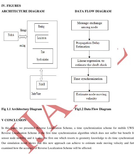
IV. FIGURES

ARCHITECTURE DIAGRAM

DATA FLOW DIAGRAM

Fig 1.1 Architecture Diagram

Fig1.2 Data Flow Diagram

V CONCLUSION

In this paper, we presented Reverse Localization Scheme, a time synchronization scheme for mobile UWSNs.

Reverse Localization Scheme is the first time synchronization algorithm which does not suffer but benefit from

sensor node mobility and it is also the first one which resorts to geometry knowledge to do time synchronization.

Our simulation result shows that this new approach can achieve to estimate node moving velocity and further

examined how the accuracy of Reverse Localization Scheme will be affected.

REFERENCES

[1] J. Elson, L. Girod, and D. Estrin. Fine-grained network time synchronization using reference broadcasts in

259 |

P a g e

www.ijarse.com

[2] N. Chirdchoo, W.-S. Soh, and K. C. Chua. Mu-sync: A time synchronization protocol for underwater

mobile networks 2008

[3] F. Akyildiz, D. Pompili, and T. Melodia. Underwater acoustic sensor networks: Research challenges. 2011

[4] Syed and J. Heidemann. Time Synchronization for High Latency Acoustic Networks in 2010.

[5] F. Sivrikay and B. Yener. Time synchronization in sensor networks: A survey in 2008.

[6] S. A. Saurabh Ganeriwal, Ram Kumar and M. Srivastava. Network-wide time synchronization in sensor

networks in 2002.

[7] D. K. Goldenberg, A. Krishnamurthy, W. C. Maness, Y. R. Yang, A. Young, A. S. Morse, A. Savvides,

and B. D. O. Anderson. Network localization in partially localizable networks in 2005.

[8] Novikov and A. C. Bagtzoglou. Hydrodynamic model of the lower hudson river estuarine system and its

application for water quality management in 2006.

[9] L. Hu and D. Evans. Localization for mobile sensor networks in 2009.

[10]J.-H. Cui, J. Kong, M. Gerla, and S. Zhou. Challenges: Building scalable mobile underwater wireless