Article
1
Deep Kalman Filter: Simultaneous Multi-Sensor
2
Integration and Modelling; GNSS/IMU Case Study
3
Siavash Hosseinyalamdary 1
4
1 Department of Earth Observation Science (EOS), Faculty of Geo-information Science and Earth
5
Observation (ITC), University of Twente; [email protected]; [email protected]; Tel.:
+31-6
(0)53-489-3921
7
8
Abstract: The Bayes filters, such as Kalman and particle filters, have been used in sensor fusion to
9
integrate two sources of information and obtain the best estimate of the unknowns. Efficient
10
integration of multiple sensors requires deep knowledge of their error sources and it is not trivial
11
for complicated sensors, such as Inertial Measurement Unit (IMU). Therefore, IMU error modelling
12
and efficient integration of IMU and Global Navigation Satellite System (GNSS) observations has
13
remained a challenge.
14
In this paper, we develop deep Kalman filter to model and remove IMU errors and consequently,
15
improve the accuracy of IMU positioning. In other words, we add modelling step to the prediction
16
and update steps of Kalman filter and the IMU error model is learned during integration. Therefore,
17
our deep Kalman filter outperforms Kalman filter and reaches higher accuracy.
18
Keywords: Deep Kalman Filter; Simultaneous Sensor Integration and Modelling (SSIM);
19
GNSS/IMU Integration; Recurrent Neural Network; Deep Learning; Long-Short Term Memory
20
(LSTM);
21
22
1. Problem Statement
23
Global Navigation Satellite System (GNSS) enables us to locate ourselves within a few
24
millimeters all over the world. This system consists of Global Positioning System (GPS), Galileo,
25
Glonass, and Beidu, and it is integrated in our daily life from car navigators to airplanes.
26
Unfortunately, GNSS positioning requires clear sky view and therefore, it is not available in urban
27
canyons where GNSS signals are blocked by high-rise buildings. Therefore, other alternative
28
navigation solutions are applied to overcome this shortcoming of GNSS positioning and bridge its
29
gaps in urban canyons.
30
Among alternative navigation solutions, inertial navigation and visual odometry are
cost-31
effective and they do not require any infrastructure. Inertial Measurement Unit (IMU) is a
32
composition of accelerometers and gyroscopes and it estimates position, velocity, and orientation of
33
the platform from measured accelerations and angular rates.
34
The error characteristics of IMU sensors are complicated. They significantly differ from one
35
technology, one manufacturer, and even one sensor to another. The cold atom IMUs are the most
36
accurate IMUs (Battelier 2016), but they are very expensive and they are not applied for commercial
37
applications such as mobile mapping. Other IMU technologies, such as Mechanical Gyro, Ring Laser
38
Gyro (LRG), Fiber Optic Gyro (FOG), and Micro-Electro-Mechanical System (MEMS), suffer from
39
common error sources, such as bias and scale factor errors, but some technologies have their own
40
specific error sources, such as dead zone error in RLG. MEMS sensors, which are cost-effective and
41
are frequently used in industry, suffer from various error sources and their positioning accuracy
42
quickly deteriorates in the absence of GNSS positioning.
43
The IMU sensors have systematic, random, and computational error sources. The IMU
44
manufacturers use controlled environments, such as turntable, to estimate and remove systematic
45
errors. The calibration procedure using controlled environment is costly and it cannot fully remove
46
systematic errors. Some random errors, such as run-to-run bias, are added to the state vector and are
47
estimated and removed from IMU observations when GNSS positioning is available. Therefore, these
48
error sources should be modelled. The true nature of these errors is very complicated and it depends
49
on many unobserved parameters, such as temperature.
50
In contrast, the Bayes estimators, such as the Kalman and Particle filters, have many limitations
51
and they may not be able to model the IMU errors. In the Kalman filter, the error model should linear
52
with Gaussian distribution and therefore, they are not very useful for the IMU error modeling.
53
Particle filter can handle non-linear IMU error models with non-Gaussian distribution. However,
54
particle filter is applicable when the IMU error model and its data distribution are known.
55
If the error characteristics of IMU sensors can be accurately modelled, its accuracy is significantly
56
improved. Currently, scientists suggest different error models for IMU error sources separately. For
57
instance, Jekeli (2001) has suggested to model the bias of accelerometer and gyroscope as random
58
constant and Noureldin et al. (2013) has applied first-order Gauss-Markov stochastic process to
59
model these biases.
60
In this paper, we introduce deep Kalman filter to simultaneously integrate GNSS and IMU
61
sensors and model the IMU errors. In contrast to previously proposed approaches, our approach does
62
not have any pre-defined IMU error model and it is learned from observations. Therefore, we do not
63
need to assume any stochastic or deterministic behavior of IMU errors. In contrast to previously
64
proposed approaches, we can accurately model the non-linear, time-variant, highly correlated IMU
65
error sources.
66
1.1. Literature Review
67
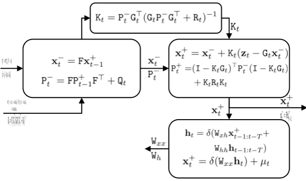
There are a few scientific endeavors to harness the IMU errors and provide accurate alternative
68
positioning system in the absence of GNSS positioning. We have already discussed that bias of
69
accelerometer and gyro is modelled as random constant in Jekeli (2001) and it is modelled as
first-70
order Gauss-Markov stochastic process in Noureldin et al. (2013). Shin and El-Sheimy (2002) use
71
gravity and earth rotation rate to calibrate the IMU errors.
72
Wang et al. (2016) treat the IMU error sources as time series and apply the AutoRegressive and
73
Moving Average (ARMA) to model the IMU error sources. In addition to the statistical estimators,
74
shallow Multi-Layer Perceptron (MLP) network have been utilized to model IMU error sources in
75
the presence of GNSS positioning (Chiang et al. 2008, Noureldin et al. 2011). Adaptive Neural Fuzzy
76
Information Systems (ANFIS) has also applied to capture the IMU uncertainties (Abdel-Hamid et al.
77
2007, Zhang et al. 2014). Toth and his colleagues have applied neural networks and fuzzy logic (Toth
78
et al. 2007) to model the IMU error sources. Navidi et al. (2015) use hybrid Fuzzy Inference System
79
(FIS) and second-order extended Kalman filter to integrate GNSS and IMU sensors. Xing and his
80
colleagues have showed that chaotic particle swarm optimization significantly reduces the gyroscope
81
random drift (Xing et al 2017). The applied neural networks are shallow and they do not accurately
82
calibrate IMU since they do not consider the IMU’s correlation over time. In other words, IMU error
83
sources should be studied as a time series and model the IMU error sources over time.
84
It has been shown that the shallow neural networks can only model simple phenomena and the
85
complicated systems should be modelled using deep neural network (Minsky and Papert 1988).
86
Therefore, we apply deep neural network for sensor integration. Up to our knowledge, we are the
87
first who apply deep neural network for GNSS and IMU integration and IMU error modelling.
88
Mirowski and Lecun (2009) have introduced dynamic factor graphs and reformulated the Bayes
89
filters as recurrent neural networks. In their proposed approach, the observation and system models
90
of the Kalman filter are learned from observations. Gu et al. (2017) reformulate Kalman filter and
91
recurrent neural network to model face landmark localization in videos. Krishnan et al. (2015)
92
integrate Kalman filter and variation methods for learning famous machine learning dataset, MNIST.
93
2. Kalman filter
95
The unknown vector, which is estimated in the Kalman filter, is called state vector and it is
96
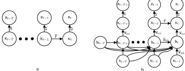
represented by , where t indicates to the state vector at time t. It also depends on the
97
observation vectors, , where , and the initial state of the system . The probability of state
98
vector at the current time is . Therefore, the current state vector is estimated using
99
Maximum Likelihood (ML), such that:
100
(1) The probability of current state vector depends on the previous state vectors, such that
101
(2)
The denominator in Equation (2) is a normalization constant and it does not contribute in
102
maximization of likelihood in Equation (2), such that:
103
(3) The state vector at current time directly depends on the previous state vectors. Therefore, the
104
marginalization of previous state vectors is applied, such that:
105
(4)
Based on Markovian assumption, the state vector at the current time only depends on the state vector
106
at the previous time, such that:
107
(5)
where is the posterior probability estimation of the current state vector. The state vector best
108
estimate in the previous time is . Therefore, equation (5) is
109
reformulated as:
110
(6)
where is the prior probability estimation. It predicts the
111
current state vector based on the system model and the posterior estimation of state vector in the
112
previous time.
113
In the Kalman filter, the state vector is related to the state vector at the previous times,
114
using system model, , such that:
115
(7) where, , is noise of system model. The state vector relates to the observation vector, , with
116
the observation model, , such that:
117
(8) where, , is noise of observation model. The state and observation models are assumed to be linear
118
in the Kalman filter. Therefore, these functions can be replaced by and matrices, respectively.
119
The system model is rewritten, such that:
120
(9) and similarly, the observation model is rewritten, such that:
121
(10) Noise of system and observation models have Normal distribution in the Kalman filter, such that:
122
(11) (12) where and are the covariance matrices of system and observation models.
123
The Kalman filter is designed in the two-stage optimization. In the first stage, the current state
124
vector is predicted based on the state vector in the previous time, such that:
125
(13) The predicted values are represented by superscript ‘-‘ and the updated values are represented by
126
superscript ‘+’. The error propagation is applied to estimate the covariance matrix of current state
127
vector based on the covariance matrix of state vector in the previous time, such that:
128
where is the predicted covariance matrix of state vector. In the update stage of Kalman filter, the
129
current state vector is updated by using observation vector, such that:
130
(15) and the covariance matrix of updated current state vector is calculated, such that:
131
(16) where is the Kalman gain matrix and it is calculated, such that
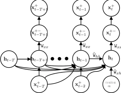
132
(17) For derivation of Kalman filter equations, reader is referred to Jeleki (2001). Figure 1 shows the
133
Kalman filter.
134
Figure 1: The Kalman filter procedure; It consists of prediction (left-up box) and update steps (right-up box).
2.1.1. Shortcoming of Kalman filter
135
There are a number of shortcomings in Kalman filter: and are linear models with Gaussian
136
noise. Therefore, they cannot model non-linear functions or linear functions with non-Gaussian noise.
137
In addition, these functions are time invariant and they do not change over time. A number of
138
variations in Kalman filter, such as extended and unscented Kalman filters, can handle non-linear
139
observation and system models. In addition, particle filter works on the observation and system
140
models with other distributions than Gaussian noise.
141
Nonetheless, the observation and system models of Bayes filters should be known. In other
142
words, scientists should find a model to relate state vectors to observations and the dynamic of the
143
system. For instance, we discussed that the bias of accelerometer and gyro are modelled in different
144
ways. In addition, noise probability distribution of the observation and system model should be
145
known. Unfortunately, the observation and system models cannot be determined beforehand in
146
many applications.
147
Another shortcoming of the Bayes filters is their Markovian assumption. In Bayes filter, it is
148
assumed that the current state vector only depends on the previous state vector and it is independent
149
from older state vectors. Although, this property significantly simplifies the system model and it
150
makes these filters very efficient, it makes the Bayes filter insensitive to system behavior with longer
151
correlation time. In other words, complicated error models with long correlation time cannot be
152
modelled in Bayes filters.
153
Here, we provide our discussion with an example on our case study, IMU error modelling. The
154
IMU models have different error sources depending the technology, which is applied in their
155
accelerometers and gyroscopes. One IMU manufacturer can calibrate the IMU error sources different
156
from another manufacturer. Moreover, the error sources of MEMS sensors can significantly differ
157
from one MEMS sensor to another even in one family. The pre-defined IMU error models cannot
158
handle high variations of error sources in MEMS sensors. In addition, high correlation between
159
different MEMS error sources makes the IMU error modelling very complicated. Often, it is not
160
possible to discriminate the error sources in MEMS sensors.
161
3. Methodology
165
In this paper, we add system modelling to the Kalman filter and we call it deep Kalman filter. In
166
other words, deep Kalman filter is able to estimate the system model and it is useful in many
167
applications, such as GNSS/IMU integration, where the system model is complicated. In order to
168
estimate the system model of Kalman filter, we add latent variables to the Kalman filter. Latent
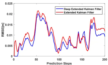
169
variables are not observed and they are invisible in the state vector, but the state vector depends on
170
the latent variables. As an example, IMU errors depend on the temperature, but it is not observed
171
and cannot be estimated. These variables are represented with the latent vector, , where the
172
subscription t stands for the latent vector in the current time.
173
We assume the current state vector, , depends on the current and previous latent vectors,
174
. Therefore, the current state vector indirectly depends on previous state vectors, , and
175
Markovian assumption does not hold anymore. We design our modelling step in the way that the
176
current state vector depends on the current latent vector and current latent vector depends on
177
previous state vectors and previous latent vectors. This is one of many different architectures of
178
possible networks, but it significantly simplifies our network.
179
Let’s assume there is a function that relates the current latent vector to the previous latent
180
vectors and previous state vectors, such that:
181
(18) and the current state vector is directly related to the current latent vector by a function, , such that:
182
(19) we name the posterior estimation based on our model as . In other words, is the predicted
183
posterior estimation of state vector. Functions and are a combination of linear and non-linear
184
functions and therefore, they can create non-linear models. The linear function has several coefficient
185
parameters, represented by coefficient matrices, , but the non-linear function, , has no parameter.
186
Therefore, our network is designed, such that:
187
(20) (21) Let’s name the parameters of latent vector, . In order to model our system, it
188
suffices to estimate and . Figure 2 shows the probabilistic graphical model of Kalman filter
189
and deep Kalman filter. The upper part of deep Kalman filter is prediction and update steps and it is
190
similar to Kalman filter. However, we added modelling step to Kalman filter and it is the lower part
191
of deep Kalman filter in Figure 2.
192
a b
Figure 2: The probabilistic graphical model of Kalman filter (a) and deep Kalman filter (b).
193
When the posterior estimation of state vector is available, , it can be replaced with in
194
equation (21) and the latent vector and the coefficient matrix, , are estimated. In order to estimate
195
the latent vector, we use maximum likelihood estimation. In other words, we maximize the likelihood
196
of latent vector, such that:
197
Instead of latent vector estimation, it suffices to estimate coefficient matrix, . By replacing latent
198
vector from equation (20) into equation (22), it is reformulated as:
199
(23) The latent vector on the left side depends on the coefficient matrix, , in the right side, which is
200
also unknown. Therefore, we utilize expectation-maximization iterative method to estimate all
201
coefficient matrices, and consequently model our system.
202
In the expectation maximization, we first assume there is an initial guess for our coefficient
203
matrix . Based on the initial guess of coefficient matrix, the latent vector, , is estimated, such
204
that:
205
(24)
where superscript numbers with parenthesis indicate to iterations.
206
The new coefficient matrix of is estimated by maximizing the probability of coefficient
207
matrix based on the latent vectors, such that:
208
(25)
The iteration continues until it converges to local maximum and [ , ] and [ , ] do
209
not significantly change. When the coefficient matrices are estimated, the system model is estimated.
210
After the system model is estimated, the state vector can be predicted using the modelled system in
211
equations (20) and (21). Figure 3 shows the scheme of deep Kalman filter.
212
213
Figure 3: The deep Kalman filter procedure. The IMU modelling step (right-bottom) has been added to Kalman filter.
3.1. Recurrent Neural Network
214
The expectation maximization will lead to global maximum in the convex functions. However,
215
it is most likely it converges to local maximum, since modelling is not convex for complicated models.
216
One of the challenges is finding an approach to maximize the equations (24) and (25). This
217
maximization is equivalent to minimization of model prediction and the current state vector.
218
Therefore, we can utilize gradient descent to minimize the error in prediction using our model. In
219
order to minimize the prediction error, we define an energy function, , and minimize it, such that:
220
(26)
by replacing from equation (21), equation (26) is reformulated, such that:
221
(27)
Therefore, the gradient of coefficient matrix, , is calculated, such that:
222
The gradient of latent vector coefficient matrix, , is also estimated, such that:
223
(29)
Therefore, the coefficient matrices of modelled system, and , are estimated in the iterative
224
gradient descent approach, such that:
225
(30)
(31)
where is the learning rate. When the coefficient matrices are determined and system model is
226
learned, can be estimated based on previous state vectors, , in equations (20) and (21).
227
3.2. Long Short Term Memory
228
Recurrent neural networks have a drawback, known as exploding-vanishing gradient problem
229
(Goodfellow et al. 2016). When T is large and we model the system for a long time span, the gradients
230
are multiplied in several layers. If the gradients are large, their multiplication becomes humongous
231
and their gradient explodes. In the contrary, if the gradients are small, their multiplication becomes
232
insignificant, known as vanishing gradient. In order to prevent such an effect in recurrent neural
233
networks, Long Short Term Memory (LSTM) has introduced gated memories (Hochreiter and
234
Schmidhuber 1997). In LSTM, the network consists of cells and each cell can memorize the previous
235
state vectors, using input gate, remember them, using output gate, and forget them, using forget gate.
236
Let’s represent input gates as , output gates as , , and forget gates as . They are represented by
237
a combination of linear and non-linear functions, such that:
238
(32) (33) (34) where is the non-linear function and the linear functions are represented by coefficient matrices,
239
, , and . The cell state, , and hidden layer, , are estimated, such that:
240
(35) (36) where is Hadamard product. For long term correlation, input gate can keep information from
241
previous state vectors and the gradients of previous state vectors are accessible. Therefore, the
242
gradients do not explode or vanish in the back-propagation process. The forget gate controls the
243
complexity of the model and it removes the uncorrelated previous state vectors.
244
4. Implementation
245
In this chapter, we explain the details of our implementation. It has been shown that the Kalman
246
filter works better on IMU errors instead of IMU output (Jekeli 2001, Noureldin et al. 2011). Therefore,
247
we utilize the IMU mechanization to estimate position, velocity, and orientation. However, IMU
248
mechanization is not perfect and the error of position, velocity, and orientation remains in the system.
249
We define the state vector of Kalman filter consists of positioning error, velocity error, orientation
250
error, and bias of accelerometers and gyroscopes. The state vector is estimated in an extended Kalman
251
filter when GNSS observations are available and Extended Kalman filter predicts the state vector in
252
the absence of GNSS signals. The system model utilized in the Kalman filter is similar to Noureldin
253
et al. (2011).
254
When GNSS signals are available the posterior estimation of state vectors, , is calculated. Since
255
we use Real-Time Kinematic (RTK) technique for GNSS observation, our posterior estimation will be
256
very accurate and it can be used as ground truth for our IMU error modelling. Let’s call the predicted
257
posterior estimation of IMU errors using our modelling approach as . We try to predict as
258
close as possible to and therefore, we get the best estimate of modelled IMU errors. In other
259
words, we find a model to calculate as an approximation of in the presence of GNSS
260
accurately estimated, the predicted state vector using our model, , has higher accuracy than the
262
predicted state vector .
263
Figure 4: The IMU error modelling is reformulated as a time series prediction.
264
In order to implement an efficient predictive recurrent neural network, we have designed a
265
network with only one hidden layer while every hidden vector, ࢎ௧, contains 3000 variables, known
266
as nodes in neural network terminology. We are benefited from the mini-batch learning where the
267
sequences are added together and processed once. The batch size of our networks is 800. It speeds up
268
the learning process and improves the learning convergence. Another important factor of training in
269
recurrent neural network is the learning rate. We use 0.05 as initial learning rate with 5e-3 learning
270
rate decay. We have tried several sequence lengths and studied the impact of the sequence length on
271
accurate error modeling.
272
When GNSS observations are not available, the posterior estimation of state vector cannot be
273
calculated. Therefore, is not estimable and we can only predict the state vector. There are two
274
ways to predict the current state vector: using system model of Kalman filter or applying the
275
modelled system model of IMU in the deep Kalman filter. We anticipate modelled system in the deep
276
Kalman filter has better performance over system model of Kalman filter. In other words, the
277
modelled IMU errors should be more accurate than the predicted IMU errors of Kalman filter.
278
5. Experiment
279
In order to evaluate our proposed approach, KITTI benchmark (Geiger et al. 2013) has been
280
utilized. This benchmark contains multi-sensor datasets and labeled information. Among various
281
sensors, GPS and IMU information have been used in this paper. We use the longest KITTI dataset,
282
dataset No. 34, collected on October 3, 2011. This dataset contains 7:46 minutes of data collection,
283
mostly driven in residential area with clear sky view. The trajectory of platform exceeds 1.7
284
kilometers, as shown in Figure 5. The OXTS RT 3003 navigation system has been applied to collect
285
the GPS and IMU information. The GPS and IMU have already been synchronized and have been
286
collected in 10 Hz. Manufacturers have performed calibration procedure and the calibration
287
parameters, such as level-arm, are internally applied to transfer GPS information into the IMU local
288
frame. The dual-frequency RTK has been used to estimate accurate position of IMU with the accuracy
289
better than 10 centimeters.
290
We use the GPS observations as ground truth to train our network and model the IMU errors.
291
When the weights of our network are learned and IMU errors are modelled, we estimate the IMU
292
errors in two ways and compare them: First, we do not use GPS observations and we use different
293
approaches to predict IMU errors and correct IMU Positioning. Second, we use GPS observations and
294
calculate the IMU errors. The calculated IMU errors using GPS observations are utilized to correct
295
IMU positioning and we use it as baseline to evaluate the corrected IMU positioing without using
296
GPS observations.
297
Figure 5: The trajectory of KITTI dataset, #34. It is the longest KITTI dataset where the vehicle travels more than 1.7 kilometers.
6. Results
299
In order to evaluate the results, we divide the trajectory into two parts, one for training and
300
calibration and one for testing and evaluation. In the training phase, the parameters of system model
301
are estimated in the extended Kalman filter, as described in Noureldin et al. (2011). In the deep
302
extended Kalman filter, IMU errors are modelled in addition to the prediction and update stages. In
303
other words, we train our network to predict the posterior estimation of IMU errors using recurrent
304
neural network and consequently, model the IMU errors. When the network is trained, we should be
305
able to predict the posterior estimation of IMU errors and correct the IMU positioning.
306
In the testing part, we estimate the IMU errors using GNSS observations and correct the IMU
307
positioning. We utilize the corrected IMU positioning as ground truth. The extended Kalman filter
308
and deep extended Kalman filter are applied to predict the IMU errors without using GNSS
309
observations and correct the IMU positioning. The corrected IMU positioning using these two
310
approaches are compared with the ground truth and the IMU positioning error is calculated. The
311
Root Mean Square Error (RMSE) of IMU positioning is applied to evaluate the results of extended
312
Kalman filter and deep extended Kalman filter.
313
In the first experiment, we used simple RNN to predict the IMU errors and remove them from
314
the IMU positioning. In this experiment, we study the performance of extended Kalman filter and
315
deep extended Kalman filter using different sequence lengths. In other words, the sequences of IMU
316
errors, utilized to predict the IMU errors in the RNN have different lengths. We have plotted the
317
RNN in Figure 6 for the sequence length of 10, 20, and 50.
318
319
a) simple RNN with sequence length of 10
b) simple RNN with sequence length of 20
c) simple RNN with sequence length of 50
Figure 6: The RMSE of deep extended Kalman filter and extended Kalman filter (Hosseinyalamdary and Balazadegan 2017); We used different sequence lengths of simple RNN for IMU modelling of deep extended Kalman filter.
320
Figure 6 shows that the performance of RNN depends on the sequence length of previous state
321
vectors. If the sequence length is large, the network uses more IMU errors in the previous time. In
322
other words, the network applies more heuristics to predict the IMU errors and remove them from
323
IMU positioning. Therefore, the RMSE of deep Extended Kalman filter is less than the RMSE of
324
Despite of the effectiveness of RNN in the prediction of IMU errors in short period, it cannot
326
predict IMU errors in the long period of time. In other words, the RMSE of deep extended Kalman
327
filter is lower than the RMSE of extended Kalman filter in earlier time, but two approaches have the
328
same RMSE in longer period of time. This effect is due to vanishing-exploding gradient problem of
329
RNN. This well-known problem of RNN, has overcome by the development of Long Short Term
330
Memory (LSTM). LSTM uses memory gates to remember to previous IMU errors and prevents
331
repetitive gradient multiplications.
332
Figure 7 shows the IMU positioning using LSTM network with the sequence length of 10. In othr
333
words, instead of using RNN to predict IMU errors, we use LSTM to predict IMU errors and remove
334
them from IMU positioning. The sequence length of this network is similar to Figure 6a. However,
335
the effectiveness of this network does not disappear in the longer period of time. In Figure 7, deep
336
extended Kalman filter outperforms the extended Kalman filter for most of the time. There are
337
instances that extended Kalman filter has better accuracy than the deep extended Kalman filter, but
338
they are limited to few small instances. The total RMSE of deep extended Kalman filter is 0.0100
339
meters and the total RMSE of extended Kalman filter is 0.0114 meters for 20 seconds. In summary,
340
deep extended Kalman filter has better accuracy over extended Kalman filter.
341
Figure 7: The RMSE of deep extended Kalman filter and extended Kalman filter; deep extended Kalman filter IMU modelling is based on LSTM with sequence length of 10.
7. Conclusions
342
In this paper, we have introduced deep Kalman filter to estimate the system model of Kalman
343
filter. In other words, in addition to the prediction and update steps of the Kalman filter, we have
344
added modelling step to the deep Kalman filter. We have applied the deep Kalman filter to model
345
the IMU errors and correct the IMU positioning. In the deep Kalman fitler, the model of IMU errors
346
is learned using Recurrent Neural Network (RNN) and Long Short Term Memory (LSTM) when
347
GNSS observations are available. The IMU errors can be predicted using learned model in the absence
348
of GNSS observations.
349
We have experimented the Kalman filter and deep Kalman filter using KITTI dataset and the
350
results show that our approach outperforms the Kalman filter. Therefore, we reach better accuracy
351
in the deep Kalman filter. In addition, deep Kalman filter using RNN can predict the IMU errors for
352
short period of time, but its effectiveness disappears in longer period of time due to its
vanishing-353
exploding gradient problem. Deep Kalman filter based on Long Short Term Memory (LSTM) have
354
better accuracy over Kalman filter and it can predict IMU errors in longer period of time.
355
References
356
1. Jekeli C. (2001), Inertial Navigation Systems with Geodetic Applications, Walter de Gruyter.
357
2. Noureldin A., Karamat T.B., Georgy J. (2013), Fundamentals of Inertial Navigation, Satellite-based
358
Positioning and their Integration, Springer-Verlag Berlin Heidelberg.
359
3. Shin E.-H. and El-Sheimy N. (2002), A new calibration method for strap down inertial navigation systems.
360
Zeitschrift f ̈ur Vermessungswesen, 127 (1), 1–10.
361
4. Wang, S., Deng, Z., & Yin, G. (2016), An Accurate GPS-IMU/DR Data Fusion Method for Driverless Car
362
5. Chiang K.W., Noureldin A., El-Sheimy N. (2008), Constructive Neural-Networks-Based MEMS/GPS
364
Integration Scheme, in IEEE Transactions on Aerospace and Electronic Systems, vol. 44, no. 2, pp. 582-594.
365
6. Noureldin A., El-Shafie A., Bayoumi M. (2011), GPS/INS Integration Utilizing Dynamic Neural Networks
366
for Vehicular Navigation, Information Fusion 12 (1), pp. 48-57.
367
7. Abdel-Hamid W., Noureldin A., El-Sheimy N., (2007), Adaptive Fuzzy Prediction of Low-Cost
Inertial-368
Based Positioning Errors, in IEEE Transactions on Fuzzy Systems, vol. 15, no. 3, pp. 519-529.
369
8. Zhang L., Liu J., Lai J., Xiong Z., (2014) Performance Analysis of Adaptive Neuro Fuzzy Inference System
370
Control for MEMS Navigation System, Mathematical Problems in Engineering, Vol 2014.
371
9. C. Toth, D. A. Grejner-Brzezinska, and S. Moafipoor, “Pedestrian Tracking and Navigation Using Neural
372
Networks and Fuzzy Logic,” in 2007 IEEE International Symposium on Intelligent Signal Processing. IEEE,
373
2007, pp. 1–6.
374
10. Navidi N., Landry R.J., Cheng J., Gingras D. (2016), A New Technique for Integrating MEMS-Based
Low-375
Cost IMU and GPS in Vehicular Navigation, Journal of Sensors, Vol 2016.
376
11. Xing H., Hou B., Lin Z., Guo M. (2017), Modeling and Compensation of Random Drift of MEMS Gyroscopes
377
Based on Least Squares Support Vector Machine Optimized by Chaotic Particle Swarm Optimization,
378
Sensors, 17(10).
379
12. Minsky M.L. and Papert S.A. (1988), Perceptrons: Expanded Edition. MIT Press, Cambridge, MA, USA.
380
13. Mirowski P. and Lecun Y. (2009), Dynamic Factor Graphs for Time Series Modelling, In Machine Learning
381
and Knowledge Discovery in Databases - European Conference, ECML PKDD, Vol. 5782 LNAI, pp.
128-382
143.
383
14. Gu J., Yang X., De Mello S., Kautz J. (2017), Dynamic Facial Analysis: from Bayesian Filtering to Recurrent
384
Neural Network, IEEE Conference on Computer Vision and Pattern Recognition (CVPR), pp. 1531-1540.
385
15. Krishnan R.G., Shalit U., Sontag D. (2017), Structured Inference Networks for Nonlinear State Space
386
Models, Thirty-First AAAI Conference on Artificial Intelligence.
387
16. Goodfellow I., Bengio I., Courville A. (2016), Deep Learning, the MIT Press.
388
17. Hochreiter S. and Schmidhuber J. (1997), Long Short-Term Memory, Neural Comput. 9, 8, pp.1735-1780.
389
18. Geiger A., Lenz P., Stiller C., and Urtasun R. (2013), Vision meets Robotics: The KITTI Dataset, International
390
Journal of Robotics Research (IJRR).
391
19. Hosseinyalamdary S. and Balazadegan Y. (2017), Error Modeling of Reduced IMU using Recurrent Neural