Event Reconstruction in the Tracking System
of the CBM Experiment
VolkerFriese1,for the CBM collaboration 1GSI Darmstadt, Germany
Abstract.The Compressed Baryonic Matter experiment (CBM) will investigate strongly interacting matter at high net-baryon densities by measuring nucleus-nucleus collisions at the FAIR research centre in Darmstadt, Germany. Its ambitious aim is to measure at very high interaction rates, unprecedented in the field of experimental heavy-ion physics so far. This goal will be reached with fast and radiation-hard detectors, self-triggered read-out electronics and streaming data acquisition without any hardware trigger. Collision events will be reconstructed and selected in real-time exclusively in software. This puts severe requirements to the algorithms for event reconstruction and their implementation. We will discuss some facets of our approaches to event reconstruction in the main tracking device of CBM, the Silicon Tracking System, covering local reconstruction (cluster and hit finding) as well as track finding and event definition.
1 Introduction
The CBM (“Compressed Baryonic Matter”) experiment is a dedicated heavy-ion experiment which will be operated at the FAIR facility currently under construction in Darmstadt, Ger-many [1]. CBM will investigate collisions of heavy nuclei in the beam momentum range
pbeam=3.5 – 12 GeV/nucleon, with the aim to study strongly interacting matter at extreme net-baryon densities [2, 3]. The experimental setup comprises a variety of detector systems arranged in a typi-cal fixed-target geometry (Fig. 1, left): a tracking system (STS) build of silicon micro-strip detectors located inside a dipole magnet for the momentum determination, a time-of-flight detector (TOF) for identification of direct hadrons, a ring-imaging Cherenkov detector (RICH) and a transition-radiation detector (TRD) for the identification of electrons, and a forward calorimeter (PSD) for event charac-terisation. The RICH can be replaced by an active absorber system for muon identification (MUCH). The worldwide interest in the study of dense QCD matter is currently reflected by a number of experimental programmes for nuclear collisions at moderate beam energies, such as the beam-energy scan programme at RHIC, the NA61 experiment at CERN, and planned new facilities in Germany, Russia, China and Japan [4]. Among these, CBM is unique in its ambitious goal to measure at very high interaction rates of up to 107 collisions per second, more than two orders of magnitude higher than other running or planned experiments. Such interaction rates would give access to extremely rare observables like, e.g., multi-strange anti-hyperons or charmed hadrons. This design goal implies enormous challenges not only to the detectors and read-out electronics in terms of speed and radiation
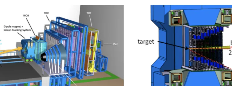
Figure 1.(Colour online) Left: Setup of the CBM experiment. The beam extracted from the synchrotron enters from the left. Inside the superconducting dipole magnet, the target, the Micro-Vertex Detector and the Silicon Tracking System are located. Further downstream are the Ring-Imaging Cherenkov Detector (RICH) and the Transition-Radiation Detector (TRD), both for electron identification. The TOF wall serves hadron identification by time-of-flight measurement. The setup is concluded by the Projectile Spectator Detector (PSD), a forward calorimeter for event characterisation in terms of centrality and reaction plane angle. Right: The Silicon Tracking System inside the aperture of the magnet. About 900 double-sided silicon micro-strip sensors are arranged in eight stations for track reconstruction.
hardness, but also to the data acquisition system and data processing [5, 6]. The readout concept of CBM foresees no hardware trigger at all; instead, autonomous front-end electronics will deliver time-stamped hit messages on activation by a charged particle crossing the respective detector element. The full detector information is aggregated by the DAQ and delivered to an online compute cluster. Here, the raw data will be inspected in real time, and event data containing signatures of rare observables will be selected for storage. The challenge is to reduce the raw data rate of about 1 TB/s to an archival rate of several GB/s, thus by a factor of 300 or more. The required selectivity and the complex nature of the trigger signatures necessitate almost complete reconstruction of tracks and events online.
2 Reconstruction in the CBM experiment
Reconstruction in CBM, as in all high-energy physics experiments, means establishing the particle trajectories from the measurements in the detectors, and the determination of the event vertex. These entities are then subjected to higher-level physics analysis, either offline or in real time during the experiment operation. An “event” here means a collection of data presumably belonging to one colli-sion. A reconstructed event is a collection of tracks (trajectories) originating from a common vertex. The number of charged particles created in a typical heavy-ion collision at CBM energies is about 1,000, out of which up to 500 are covered by the detector acceptance. Thus, reconstruction has to deal with very complex event topologies.
Figure 1.(Colour online) Left: Setup of the CBM experiment. The beam extracted from the synchrotron enters from the left. Inside the superconducting dipole magnet, the target, the Micro-Vertex Detector and the Silicon Tracking System are located. Further downstream are the Ring-Imaging Cherenkov Detector (RICH) and the Transition-Radiation Detector (TRD), both for electron identification. The TOF wall serves hadron identification by time-of-flight measurement. The setup is concluded by the Projectile Spectator Detector (PSD), a forward calorimeter for event characterisation in terms of centrality and reaction plane angle. Right: The Silicon Tracking System inside the aperture of the magnet. About 900 double-sided silicon micro-strip sensors are arranged in eight stations for track reconstruction.
hardness, but also to the data acquisition system and data processing [5, 6]. The readout concept of CBM foresees no hardware trigger at all; instead, autonomous front-end electronics will deliver time-stamped hit messages on activation by a charged particle crossing the respective detector element. The full detector information is aggregated by the DAQ and delivered to an online compute cluster. Here, the raw data will be inspected in real time, and event data containing signatures of rare observables will be selected for storage. The challenge is to reduce the raw data rate of about 1 TB/s to an archival
rate of several GB/s, thus by a factor of 300 or more. The required selectivity and the complex nature
of the trigger signatures necessitate almost complete reconstruction of tracks and events online.
2 Reconstruction in the CBM experiment
Reconstruction in CBM, as in all high-energy physics experiments, means establishing the particle trajectories from the measurements in the detectors, and the determination of the event vertex. These entities are then subjected to higher-level physics analysis, either offline or in real time during the
experiment operation. An “event” here means a collection of data presumably belonging to one colli-sion. A reconstructed event is a collection of tracks (trajectories) originating from a common vertex. The number of charged particles created in a typical heavy-ion collision at CBM energies is about 1,000, out of which up to 500 are covered by the detector acceptance. Thus, reconstruction has to deal with very complex event topologies.
Owing to the free-streaming design of the CBM readout and data acquisition, the input to recon-struction is a continuous stream of detector raw data, the atomic information units being messages from a single electronic channel typically containing address, time and charge. Unlike for triggered readout systems, where the hardware trigger defines an event data set on which the reconstruction routines can operate, the raw data of CBM will not be partitioned into events. So, events as subject to physics analysis have to be established by the reconstruction procedure itself, making use of the time
information of all measurements. Reconstruction thus becomes 4-dimensional in space and time. It should be noted that a trivial decomposition of the data stream into events based on the time infor-mation of the raw data themselves is hardly possible at very high interaction rates, since the average time interval between two subsequent events is of the same order of magnitude as the time extension of a typical event; the case that events overlap in time on raw data level thus occurs rather frequently. Low-level reconstruction (cluster, hit and track finding) thus must operate on the continuous data stream.
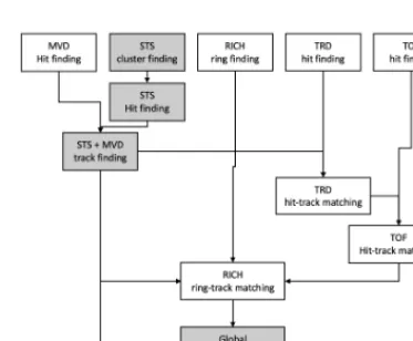
Figure 2.Schematic process graph for reconstruction in CBM. Local reconstruction provides hits (space points) in all detector systems (rings in case of the RICH detector). Tracks are first reconstructed in the STS and MVD inside the magnetic field; hits of the other detector systems are then attributed to these tracks. Tracks originating from a common vertex are grouped into events, which are then characterised by the PSD measurement in terms of centrality and event-plane angle. The procedures in the highlighted boxes are discussed in this article.
The reconstruction procedure for CBM consists of several steps. A simplified and schematic process graph is depicted in Fig. 2. The first step is local reconstruction in the various detector systems; here “local” means that reconstruction is independent from other detector elements. Charged particles typically activate not a single, but several readout channels, which represent neighbouring readout elements (pixels, strips, pads). The cluster finding procedure thus groups simultaneously activated neighbouring channels to a cluster. For CBM, “simultaneous“ means that the time difference
of the measurements in a cluster is smaller than a pre-defined threshold value, which corresponds to the time resolution of the respective detector. From a found cluster, a “hit” can be reconstructed by assigning a cluster centre position. A typical method for this is to determine a charge-weighted mean. Hits are 4-dimensional points in space-time. They are the reconstructed intersection points of the particle trajectories with active detector elements and are the input to track finding. Track finding is first performed from the measurements in the STS and MVD. From these local tracks, global tracks are formed by associating the measurements in the downstream detectors. On the basis of the reconstructed tracks, events can be defined as groups of tracks originating from a common vertex in configuration space and time.
Common for all software to be used in real-time reconstruction is the requirement to be extremely fast. CBM targets at an average event reconstruction time of 20 ms, which would result in a compute capacity of the online cluster of about 1 M HepSpec06 (about 65,000 current CPU cores). Timing performance is thus, besides efficiency and accuracy, a decisive design argument for all CBM
In the following sections, we describe some selected parts of the reconstruction graph, namely local reconstruction (cluster and hit finding) in the STS, track finding in the STS, and event finding. The reason for this choice is that these parts are some of the best established ones, and that they represent the computationally most demanding algorithms, since the track model in the magnetic dipole field is non-trivial, and track finding in the STS is a huge combinatorial problem. The STS detector [7] is an arrangement of eight stations positioned close to the target (z =30 – 100 cm) in
the aperture of the dipole magnet (Fig. 1, right). It is constructed of about 900 double-sided silicon micro-strip sensors with a strip pitch of 58µm.
3 From digis to clusters: Cluster finding in the STS
A charged particle traversing a sensor of the STS generates electron-hole pairs along its trajectory in the active material, which drift to the readout surfaces owing to the applied bias voltage (Fig. 3, left). The charges of both electrons and holes are collected on the strips into which the readout surfaces are segmented. From the figure it is obvious that, depending on the inclination of the particle trajectory with respect to the sensor surface, one or several strips will be illuminated. Even for perpendicularly impinging particles, effects like thermal diffusion and capacitive coupling of strips can cause more
than one strip to be activated. The task of the cluster finder is thus to find a group of measurements corresponding to one particle trajectory. This group will consist of neighbouring strips which are activated close in time.
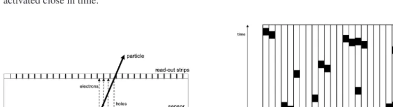
Figure 3. Left: Pictorial view of the activation of strips by a charged particle passing through a sensor of the STS. Right: Illustration of STS clusters in address (channel) space and time [8].
Were all measurements grouped into events, this task would be straightforward – all measurements could be considered simultaneous; the problem is one-dimensional and can be solved by a simple loop over the sensor channels (strips). In the real situation, however, it is not a priori known which measurement belongs to which event, and thus the time coordinate becomes essential. Clusters are now two-dimensional in the discrete address space and in the continuous time axis as illustrated in Fig. 3, right.
A straightforward approach for a 2d cluster finder, by discretizing the time axis into bins and per-forming double loops over channel and time bins, quickly runs into combinatorial problems for large data sets typically containing thousands of events. Thus, a conceptually new method was developed, which tries to accommodate the continuously streaming nature of the input data. The cluster finder is described in detail in [8]; we outline here the basic idea.
In the following sections, we describe some selected parts of the reconstruction graph, namely local reconstruction (cluster and hit finding) in the STS, track finding in the STS, and event finding. The reason for this choice is that these parts are some of the best established ones, and that they represent the computationally most demanding algorithms, since the track model in the magnetic dipole field is non-trivial, and track finding in the STS is a huge combinatorial problem. The STS detector [7] is an arrangement of eight stations positioned close to the target (z =30 – 100 cm) in
the aperture of the dipole magnet (Fig. 1, right). It is constructed of about 900 double-sided silicon micro-strip sensors with a strip pitch of 58µm.
3 From digis to clusters: Cluster finding in the STS
A charged particle traversing a sensor of the STS generates electron-hole pairs along its trajectory in the active material, which drift to the readout surfaces owing to the applied bias voltage (Fig. 3, left). The charges of both electrons and holes are collected on the strips into which the readout surfaces are segmented. From the figure it is obvious that, depending on the inclination of the particle trajectory with respect to the sensor surface, one or several strips will be illuminated. Even for perpendicularly impinging particles, effects like thermal diffusion and capacitive coupling of strips can cause more
than one strip to be activated. The task of the cluster finder is thus to find a group of measurements corresponding to one particle trajectory. This group will consist of neighbouring strips which are activated close in time.
Figure 3. Left: Pictorial view of the activation of strips by a charged particle passing through a sensor of the STS. Right: Illustration of STS clusters in address (channel) space and time [8].
Were all measurements grouped into events, this task would be straightforward – all measurements could be considered simultaneous; the problem is one-dimensional and can be solved by a simple loop over the sensor channels (strips). In the real situation, however, it is not a priori known which measurement belongs to which event, and thus the time coordinate becomes essential. Clusters are now two-dimensional in the discrete address space and in the continuous time axis as illustrated in Fig. 3, right.
A straightforward approach for a 2d cluster finder, by discretizing the time axis into bins and per-forming double loops over channel and time bins, quickly runs into combinatorial problems for large data sets typically containing thousands of events. Thus, a conceptually new method was developed, which tries to accommodate the continuously streaming nature of the input data. The cluster finder is described in detail in [8]; we outline here the basic idea.
The algorithm keeps track of the current state of the sensor in the sense that for each channel, the time of the last measurement and a link to the measurement itself are buffered. All incoming digis are
processed one after the other. If in its channel or one of the neighbouring channels a digi is found, and the time difference of the old and new measurement is above a threshold value, the corresponding
cluster is created, the channels contributing to the cluster are cleared from the buffer, and the new
digi is added to the buffer. If, on the other hand, a neighbouring channel is found active, and the time
difference is below the threshold, the new digi is added to the buffer, thus forming a cluster with the
previous measurement. At the end of processing a data portion (time-slice), clusters are formed from the remaining digis in the buffer.
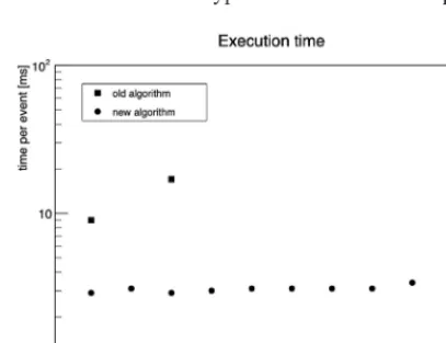
This algorithm does not involve any loop over detector channels and is thus very fast – about 3 ms per average event including the determination of the cluster centre (see section 4), which takes about 50 % of the processing time. Moreover, the execution time per event is independent from the input data size as shown in Fig. 4, whereas the previous approach with 2d cluster finding shows the factorial dependence of execution time with data size typical for combinatorial problems.
Figure 4.Execution time of the STS cluster finder (including the determination of the cluster centre) as function of the input data size (number of events processed at a time). For comparison, the squared symbols show the respective values for an older, 2-dimensional cluster finding approach. The measurements were performed on an Intel I7-4870HQ processor, 2.5 GHz, 6 MB L3 cache. Figure taken from [8].
4 Determining the cluster position
Having found a cluster consisting of a number of strips, each with a charge measurement, the question arises which coordinate across the strips to assign to the cluster. This cluster centre position and its error will enter the coordinates of the hit (see section 5) and is of importance for the track finding procedure which relies on accurate estimates of the hit position and errors.
The usual answer to this question is: if the cluster consists of one strip only, assign the strip centre as coordinate; the error is the strip pitch divided by √12. If the cluster has more than one strip, take the charge-weighted mean of the strip centre coordinates; the error is somewhat smaller than the strip pitch divided by √12. We did not find this answer satisfactory and thus tried to investigate the problem in more detail [9]. It can be formulated in a rather generic way: given a continuous distributionq(x) which is integrated in discrete bins (histogrammed) into a set of values{qi}, is there
a prescriptionxc= f({qi}) which reproduces on average the first moment ofq(x), and what is its error
(second moment)?
• If the shapeh(x) ofq(x) is known, i.e.,q(x)=Q h(x−x0), thenx0can be reconstructed with arbitrary accuracy.
• Any prescriptionxcwill have a deterministic residualδx=xc−x0which is a function only of the position ofx0relative to the centre of the binx0falls into:r=x0−xi.
• We can define an errorσxif we assume r to be randomly distributed. It is then the second moment
of the distribution ofδx. Note that in general,δxwill not be Gaussian-like distributed, since the
conditions for the Central Limit Theorem are not fulfilled.
• The prescriptionxcis unbiased, i.e., the first moment ofδxvanishes, if and only ifδx(r)=δx(−r).
This is in general not the case for the weighted mean.
For our case, we can approximateq(x) by a constant distribution:q(x)=QΘ(∆−|x−x0|), with the half-width∆given by the track inclination and the sensor thickness (see Fig. 3, right). This neglects the effects of non-uniform ionisation along the trajectory, charge diffusion and cross-talk. We can further assumerto be flatly distributed within the central strip, since the track density does not vary over the strip extension of only 58µm. In addition, the distribution of∆can be assumed to be flat, which is substantiated by detector simulations. Under these conditions, we arrive at the following definition of cluster centres and their errors:
• For one-strip clusters, the cluster centre is the centre of the strip: xc=xi. The error isσx=p/√24,
withpbeing the strip pitch. Note that the error is a factor of √2 smaller than the usually given one. • For two-strip clusters, the cluster position and its error are
xc=12(x1+x2)+p3max(q2−qq1
1,q2); σx=
p
√ 72
q2−q1 max(q1,q2).
Here,xiis the centre position andqithe charge of stripi.
• Forn-strip clusters (n≥2), the centre coordinate is
σx= 1 2
x1+xn+p·qn−q1
q
withqbeing the charge in the central strips. This prescription is accurate; the position error is zero. In all cases, the time coordinate of the cluster is calculated as the average of the times of the contributing digis, independent of their charge.
5 From clusters to hits: Hit finding in the STS
A hit as a space point is derived from the combination of a cluster on the front side of the sensor with a cluster from its backside. The strips on both sides have a relative angle, which allows to retrieve two-dimensional coordinates from the two one-dimensional measurements as illustrated in Fig. 5, left. The problem is deterministic and purely trigonometrical. The errors of the cluster positions are propagated to the errors of the hit coordinates. Thezcoordinate of the sensor itself provides the third component of the three-dimensional space point. The time associated to the hit is the average of the two cluster times.
• If the shapeh(x) ofq(x) is known, i.e.,q(x)=Q h(x−x0), thenx0can be reconstructed with arbitrary
accuracy.
• Any prescriptionxcwill have a deterministic residualδx= xc−x0which is a function only of the
position ofx0relative to the centre of the binx0falls into:r=x0−xi.
• We can define an errorσxif we assume r to be randomly distributed. It is then the second moment
of the distribution ofδx. Note that in general,δxwill not be Gaussian-like distributed, since the
conditions for the Central Limit Theorem are not fulfilled.
• The prescriptionxcis unbiased, i.e., the first moment ofδxvanishes, if and only ifδx(r)=δx(−r).
This is in general not the case for the weighted mean.
For our case, we can approximateq(x) by a constant distribution:q(x)=QΘ(∆−|x−x0|), with the
half-width∆given by the track inclination and the sensor thickness (see Fig. 3, right). This neglects
the effects of non-uniform ionisation along the trajectory, charge diffusion and cross-talk. We can
further assumerto be flatly distributed within the central strip, since the track density does not vary over the strip extension of only 58µm. In addition, the distribution of∆can be assumed to be flat,
which is substantiated by detector simulations. Under these conditions, we arrive at the following definition of cluster centres and their errors:
• For one-strip clusters, the cluster centre is the centre of the strip:xc=xi. The error isσx=p/√24,
withpbeing the strip pitch. Note that the error is a factor of √2 smaller than the usually given one.
• For two-strip clusters, the cluster position and its error are
xc=12(x1+x2)+p3max(q2−qq1
1,q2); σx=
p
√
72
q2−q1
max(q1,q2).
Here,xiis the centre position andqithe charge of stripi. • Forn-strip clusters (n≥2), the centre coordinate is
σx= 1
2
x1+xn+p·qn−q1
q
withqbeing the charge in the central strips. This prescription is accurate; the position error is zero. In all cases, the time coordinate of the cluster is calculated as the average of the times of the contributing digis, independent of their charge.
5 From clusters to hits: Hit finding in the STS
A hit as a space point is derived from the combination of a cluster on the front side of the sensor with a cluster from its backside. The strips on both sides have a relative angle, which allows to retrieve two-dimensional coordinates from the two one-dimensional measurements as illustrated in Fig. 5, left. The problem is deterministic and purely trigonometrical. The errors of the cluster positions are propagated to the errors of the hit coordinates. Thezcoordinate of the sensor itself provides the third component of the three-dimensional space point. The time associated to the hit is the average of the two cluster times.
It should be noted that the construction of hits from the projective strip geometry leads to ambi-guities in case of several clusters being present in a sensor at a time (see Fig. 5, right). Depending on the track density, the so-called fake hits can outnumber the real hits; in a typical CBM situation, their amount is approximately equal to that of true hits. The fake hits are the price to pay for having a strip readout instead of a pixel readout and constitute an additional challenge for the track finding procedure.
Figure 5.Hit finding in the STS. Left: a hit is defined by the intersection of a front–side cluster with a back-side cluster, having a relative stereo angleΦ. Each cluster is characterised by the centre position and its error. These
define an overlap region, from which the hit position and its errors inxandyare determined. Right: Fake hits
produced by the presence of several active clusters.
6 From hits to tracks: Track finding in the STS
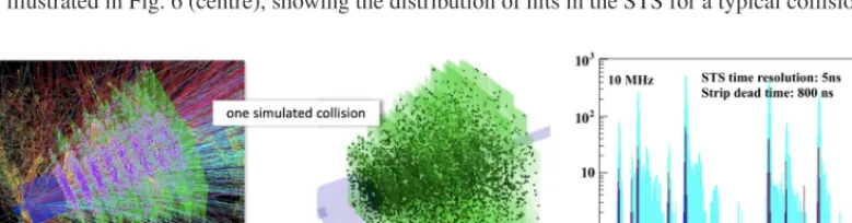
Track finding is usually the most involved problem in the reconstruction of high-energy physics ex-periments. This holds in particular for heavy-ion experiments with a large number of particles being produced in each collision, which results in highly occupied detectors. In fixed-target experiments like CBM, the kinematic forward focusing due to the Lorentz boost creates a highly inhomogeneous hit density, with highest value in the inner parts of the detectors close to the beam pipe. The situation is illustrated in Fig. 6 (centre), showing the distribution of hits in the STS for a typical collision.
Figure 6. (Colour online) Left: Particle trajectories of a typical collision (central Au+Au at pbeam = 12 GeV/nucleon) simulated in the CBM-STS detector system. Centre: Resulting distribution of reconstructed
hits in the STS. Right: Time distribution of reconstructed tracks (dark) and raw data (digis, light) for simulated data (Au+Au collisions atpbeam=10 GeV/nucleon) at 10 MHz interaction rate.
suitable three-dimensional grids (one per detector station) for fast look-up. These extensions of the original algorithm do not affect the reconstruction efficiency even at the highest interaction rates; it is about 98 % for primary tracks withp>1 GeV.
7 From tracks to events: Event finding
With reconstructed tracks, it is finally possible to define events. The reasons for this are twofold: first, the track time is better defined than the single measurement time, because through the chain clusters – hits – tracks, the tracks consists of a number of digis – at least eight. Second, track finding effectively filters out hits from late spiraling electrons created by the interaction of particles in the target or detector materials. A simple peak-finding procedure in the time distribution of reconstructed tracks allows to group them into events as shown in Fig. 6, right. With this method, 99 % of all events can be resolved at 1 MHz interaction rate, and 80 % at 10 MHz. It is currently under investigation how the remaining “pile-up” events can be resolved or at least tagged. Possible handles for this would be the time structure of tracks within the event, or the detection of multiple primary vertices within the pile-up.
8 Summary
We have briefly described some aspects of the reconstruction of tracks and events in the Silicon Track-ing System of the CBM experiment. From a stream of detector raw data, we have arrived at a set of events and associated tracks, which can be subjected to higher-level physics analysis. This is, of course, not the end of the story. Many aspects of the full event reconstruction, in particular the as-sociation of measurements from the downstream detectors, decisive for particle identification, have not been touched in this report. These are indispensable for the realisation of the physics programme of CBM, and work is continuing to bring them to a level comparable to the algorithms described in this report. However, since the computational problems discussed here are the most challenging in the reconstruction chain, we hope having demonstrated that the goal of the CBM experiment – reconstruction and selection of complex events in real time with very fast algorithms – is in reach.
References
[1] www.fair.center.eu
[2] P. Senger, N. Herrmann, Nucl. Phys. News28, 23 (2018)
[3] T. Ablyazimovet al.(CBM collaboration), Eur. Phys. J.A 53, 60 (2017) [4] V. Friese, PoS (CORFU2018) 186 (2018) pp. 1–14
[5] V. Friese,Computational Challenges for the CBM Experiment, in: Lecture Notes in Computer Science, vol 7125. Springer, Berlin, Heidelberg (2012) pp. 17–27
[6] V. Friese (for the CBM collaboration), J. Phys. Conf. Ser.898, 112003 (2017) [7] J. Heuser, V. Friese, Nucl. Phys.A 931, 1136 (2014)
[8] V. Friese, EPJ Web Conf.214, 01008 (2019)
[9] H. Malygina,Hit reconstruction for the Silicon Tracking System of the CBM experiment, Doc-toral Thesis, Goethe-Universität Frankfurt (2018)
[10] I. Kisel, Eur. Phys. J. Web Conf.95, 01007 (2015)