Statistical and Algebraic Properties of DES

Stian Fauskanger1and Igor Semaev2

1 _{Norwegian Defence Research Establishment (FFI), PB 25, 2027 Kjeller, Norway} 2

Department of Informatics, University of Bergen, Bergen, Norway

Abstract. D. Davies and S. Murphy found that there are at most 660 different probability distributions on the output from any three adjacent S-boxes after 16 rounds of DES [5]. In this paper it is shown that there are only 72 different distributions for S-boxes 4, 5 and 6. The distribu-tions from S-box triplets are linearly dependent and the dependencies are described. E.g. there are only 13 linearly independent distributions for S-boxes 4, 5 and 6. A coset representation of DES S-boxes which reveals their hidden linearity is studied. That may be used in algebraic attacks. S-box 4 can be represented by significantly fewer cosets than the other S-boxes and therefore has more linearity. Open cryptanalytic problems are stated.

Keywords: S-box · output distributions · linear dependencies· coset representation

1

Introduction

The Data Encryption Standard (DES) is a symmetric block cipher from 1977. It has block size of 64 bits and a 56-bit key. DES in its original form is deprecated due to the short key. Triple DES [1] however, is still used in many applications (e.g. in chip-based payment cards). It is therefore still important to analyze its security. DES is probably the most analyzed cipher, and is broken by linear [8] and differential [3] cryptanalysis. Even so, the most effective method in practice is still exhaustive search for the key. There are also some algebraic attacks that can break 6-round DES [4].

Donald Davies and Sean Murphy described in [5] some statistical properties of the S-boxes in DES. They found that there are at most 660 different distri-butions on the output from any three adjacent S-boxes after 16 rounds. These distributions divide the key space into classes where equivalent keys make the output follow the same distributions. The correct class is found by identifying which distribution a set of plaintext/ciphertext pairs follow. They used this to give a known-plaintext attack. The time complexity of the attack is about the same as brute-force attack and requires approximately 256.6_{plaintext/ciphertext}

pairs. The attack was improved by Biham and Biryukov [2] where the key can

?

be found with 250 _{plaintext/ciphertext pairs with 2}50 _{operations. Later,}

Kunz-Jacques and Muller [7] further improved the attack to a chosen-plaintext attack with time complexity 245_{using 2}45 _{chosen plaintexts.}

In this paper we study new statistical and algebraic properties of DES. In Section 2 we show Davies and Murphy’s results, using different notations than theirs. We also show a new exceptional property ofS4, and use this to show that

there are fewer different distributions on the output from S4S5S6 compared to

other triplets. The new properties are related to the forth S-box in DES, and is used to show that the number of different distributions on the output from S-box 4, 5 and 6 is at most 72 (after 16 rounds). This divides the key space into fewer, but larger, classes compared to Davies and Murphy’s results.

The distributions from S-box triplets are linearly dependent. We give a de-scription of the relations between the distributions, and upper bound the number of linearly independent distributions for each triplet. E.g. among the 72 different distributions for S-box 4, 5 and 6 there are only 13 linearly independent.

A coset representation of the DES S-boxes is suggested in Section 4. It is found that S-box 4 is abnormal again. It can be covered by 10 sub-cosets while the other S-boxes require at least 16. Also, the coset representation of S-box 4 contains 6 sub-cosets of size 8, while the other S-boxes contain at most one sub-coset of such size. The coset representation of S-boxes makes it possible to write the system of equations for DES in a more compact form than in [9,10].

Like the linear approximations discovered by Shamir [12] was later used by Matsui [8] to successfully break DES, these new properties might improve some attacks in the future. Two open problems are stated at the end of the paper. If solved that would improve statistical and algebraic attacks on DES.

1.1 Notations

Let Xi−1, Xi denote the input to the i-th round and Xi, Xi+1 denote the i

-th round output. So X0, X1 and X17, X16 are plaintext and ciphertext blocks

respectively, where the initial and final permutations are ignored. LetKibe the 48-bit round key at roundi. Then

Xi−1⊕Xi+1=Yi, Yi=P(S( ¯Xi⊕Ki)), (1) where ¯Xi is a 48-bit expansion of Xi, P denotes a permutation on 32 symbols, andS is a transform implemented by 8 S-boxes. LetSj be a DES S-box, so

Sj(u5, u4, u3, u2, u1, u0) = (v3, v2, v1, v0), (2)

whereui andvi are input and output bits respectively.

2

Results from Davies and Murphy

By (1), the XOR of the plaintext/ciphertext blocks are representable as follows

X17⊕X1=Y2⊕Y4⊕...⊕Y14⊕Y16, (3)

In this section we study the joint distribution of bits in X17⊕X1 and in X16⊕X0 which come from the output of 3 adjacent S-boxes in DES round

function, and therefore inYi. These results are from [5], but presented using a different notation.

2.1 Definitions and a Basic Lemma

The output of 3 adjacent S-boxes is called (Si−1, Si, Si+1)-output when i is

specified. When analysing (3) and (4) we assume the round function inputs

X2, X4, . . . , X16 and X1, X3, . . . , X15 are uniformly random and independent

respectively. Input toSi is accordingly assumed to be uniformly random. These common assumptions were already in [5].

When we look at a reduced number of rounds in DES (k rounds), then

Xk+1⊕X1andXk⊕X0follows the distribution for the XOR ofk/2 round-outputs

(for even k). We will throughout this paper use 2n to denote the number of rounds.nis the number of outputs that are XORed, and full DES is represented byn= 8.

We define three distributions that are related to each Si. We use notation (2).

1. The distribution of (u1, u0, v3, v2, v1, v0) is called right hand side

distri-butionand we denotep(y,ri) =Pr((u1, u0) =y and (v3, v2, v1, v0) =r).

2. The distribution of (u5, u4, v3, v2, v1, v0) is calledleft hand side

distribu-tionand we denoteqx,r(i) =Pr((u5, u4) =xand (v3, v2, v1, v0) =r).

3. The distribution of (u5, u4, u1, u0, v3, v2, v1, v0) is called LR distribution

and we denote

Q(x,y,ri) =Pr((u5, u4) =x, and (u1, u0) =y, and (v3, v2, v1, v0) =r).

Obviously, p(y,ri) =PxQ

(i)

x,y,r and q

(i)

x,r =PyQ

(i)

x,y,r, the sums are over 2-bit x, y respectively.

Lemma 1. For any2-bitx, yand any 4-bitrholds

p(_y⊕i)_2,r+p(_y,ri) = 1

32 , (5)

q(_x⊕i)_1,r+q(_x,ri) = 1

32 , (6)

Q_x,y,r(i) +Q(_x,y⊕i) _2,r+Q_x⊕(i)_1,y,r+Q(_x⊕i)_1,y⊕2,r= 1

64. (7)

Proof. The equalities (5) and (6) were found directly from the values ofp(y,ri), q(x,ri), for instance, see those distributions listed for S4 in Appendix 1. Alternatively,

by DES S-box definition, for any fixed (u5, u0) the distribution of (v3, v2, v1, v0)

is uniform. So (u0, v3, v2, v1, v0) and (u5, v3, v2, v1, v0) are uniformly distributed

2.2 Output-Distributions on S-box Triplets

We study the distribution of the output from three adjacent S-boxes in DES round function. Let (a5, ..., a0), (b5, ..., b0) and (c5, ..., c0) be the input to three

adjacent S-boxes in one DES round. Then

(a1, a0)⊕(b5, b4) =k and (b1, b0)⊕(c5, c4) =k0 ,

where k and k0, thecommon key bits, are both 2-bit linear combinations of round-key-bits. By kj = (kj1, kj0) and k0j = (k0j1, kj00) we denote the common

key bits in roundj.

Let (r, s, t) be a 12-bit output fromSi−1, Si, Si+1 in one DES round. Then

Pr(r, s, t|k, k0) = 24×X

x,y

p(_x⊕k,ri−1) Q_x,y,s(i) q_y⊕k(i+1)0_,t. (8)

The distribution of (r, s, t) after 2nrounds is then-fold convolution of (8):

Pr(r, s, t| k1, k10, ..., kn, kn0) = X

n Y

i=1

Pr(ri, si, ti |ki, ki0),

where the sum is over (ri, si, ti) such that Li(ri, si, ti) = (r, s, t). By changing the order of summation and using (8) we get

Pr(r, s, t|k1, k01, ..., kn, kn0) (9)

= 24n×Xp(_xi−1)

1⊕k1,...,xn⊕kn,r×Q

(i)

x1,y1,...,xn,yn,s×q

(i+1)

y1⊕k10,...,yn⊕k0n,t

,

where the sum is over 2-bitx1, y1, ..., xn, yn, and

p(_xi)

1,...,xn,r= X

L jrj=r

p(_xi)

1,r1× · · · ×p (i)

xn,rn,

q_y(i₁)_,...,yn,t= X L

jtj=t

q(_yi₁)_,t1× · · · ×q_y(i_n)_,tn,

Q(_xi)

1,y1,...,xn,yn,s= X

L jsj=s

Q(_xi)

1,y1,s1× · · · ×Q (i)

xn,yn,sn.

Lemma 1 implies the following corollary.

Corollary 1. For any 2-bit x1, y1..., xn, yn and4-bitr, t

p(_xi)

1⊕k1,...,xn⊕kn,r =p

(i)

x1⊕k10,...,xn−1⊕k(n−1)0, xn⊕2k, r,

q_y(i)

1⊕k01,...,yn⊕kn0,t=q

(i)

y1⊕2k011,...,yn−1⊕2k(0n−1)1, yn⊕k0, t

,

wherek andk0 _{are the parity of (k}

Each value for the vector (k1, k01, ..., kn, k0n) can be mapped to a distribution on (r, s, t). Many of these distributions are equal to each other. Corollary 1 is now used to give an upper bound on the number of different distributions.

First, one can permute any (kj, k0j) and (ki, k0i) and get the same distribution. Also the distribution is defined by the parity of (k11, ..., kn1) and (k010, ..., k0n0).

There are 4 values for the two parity-bits, and there are 3+_nn

combinations for the remaining 2n bits (k10, ..., kn0) and (k110 , ..., k0n1). Therefore there are

at most 4× 3+_nn

different distributions on the output from three adjacent S-boxes. Table 1 lists the maximum number of different distributions after multiple rounds. Again, 16-round DES is specified by n=8.

Table 1.Upper bound on number of different distributions for 2nrounds

n 1 2 3 4 5 6 7 8 Upper bound 16 40 80 140 224 336 480 660

3

New statistical property of

S

In this section we find an exceptional property of S4. In particular, we prove

Lemma 2, and use it to show that there are fewer different output-distributions onS4S5S6.

Lemma 2. For any2-bitx, y, aand4-bit rholds

X

h

p(4)_x⊕a,hp(4)_y⊕a,h⊕r=X h

p(4)_x,hp(4)_y,h⊕r.

Proof. By Lemma 1,p(4)_x⊕2,h+p(4)_x,h = ₃₂1 for any 2-bit xand 4-bit h. It is easy to see the lemma is true for a = 2. All other cases are reduced to a = 1 and

x=y= 0. Let

f(h) =  



0, ifh /∈ {0,6,9,15}; 1, ifh∈ {0,9};

−1,ifh∈ {6,15}.

FromS4 right hand side distribution values, see Table 5 in Appendix 1, we find

p(4)_{x⊕1, h}+p(4)_{x, h}= 1 32+

(−1)x1_f(h)

64 (10)

and then

X

h

f(h)f(h⊕r) = 4f(r), (11)

X

h

p(4)_x,h f(h⊕r) = (−1)

x1_2f(r)

for any 2-bitx= (x1, x0) and any 4-bitr. Hence

X

h

p(4)_1,hp(4)_1,h⊕r=X h

₁ 32+

f(h) 64 −p

(4) 0,h

1 32+

f(h⊕r)

64 −p

(4) 0,h⊕r = X h

f(h)f(h⊕r)

642 −2

X

h

p(4)_0,hf(h⊕r)

64 +

X

h

p(4)_0,hp(4)_0,h⊕r=X h

p(4)_0,h p(4)_0,h⊕r.

The lemma is proved.

This surprising property holds because (10), (11),(12) are true simultaneously for the right hand side distributionp(4)_x,h.

Corollary 2. For any 2-bit x1, ..., xn and4-bitr holds

p(4)_x

1⊕k1,...,xn⊕kn,r=p

(4)

x1,...,xn−1,xn⊕k,r¯ ,

wherek¯=k1⊕ · · · ⊕kn.

Proof. By Lemma 2, X

h1⊕h2=r p(4)_x

1⊕k1,h1p (4)

x2⊕k2,h2 =

X

h1⊕h2=r p(4)_x

1,h1p (4)

x2⊕(k1⊕k2),h2

for anyx1, x2, k1, k2andr. Therefore the corollary is true forn= 2. The general

case follows recursively.

3.1 The Number of Different Output-Distributions.

Davies and Murphy found that there are at most 4× 3+_nn

different distributions of the output from 3 adjacent S-boxes after 2nrounds. In this section we show (S4, S5, S6)-output has at most (8n+ 8) different distributions.

Lemma 3. Let(r, s, t)be(S4, S5, S6)-output after2nrounds. There are at most

8n+ 8 different distributions(r, s, t)can follow.

Proof. By Corollary 1 and 2 the distribution of (r, s, t) only depends onLn_j=1kj, Ln

j=1k

0

j0 and common key bits (k110 , ..., kn01), where the order of the last nbits

is irrelevant. There are n+ 1 combinations for (k0₁₁, ..., k0_n1) and 8 possible val-ues for the three parity bits. The maximum number of different distributions is therefore at most 8n+ 8 as the lemma states.

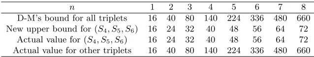
We computed the actual number of different distributions for all 8 triplets. Table 2 lists the results for n = 1, ...,8 together with the bound from Lemma 3 and Davies-Murphy’s bound. Remark that 16-round DES is specified byn= 8.

Table 2.Number of different distributions for output of 3 adjacent S-boxes

n 1 2 3 4 5 6 7 8

D-M’s bound for all triplets 16 40 80 140 224 336 480 660 New upper bound for (S4, S5, S6) 16 24 32 40 48 56 64 72

Actual value for (S4, S5, S6) 16 24 32 40 48 56 64 72 Actual value for other triplets 16 40 80 140 224 336 480 660

easier than distinguishing between many distributions (if the biases are approxi-mately the same). At the same time, the number of keys in the class representing a given distribution is larger, so more work is required to identify the correct key in the class. Also, the triplet attack described by Davies and Murphy does not perform better than the attack based on the two S-box pairs in the triplet [5]. We do not know if it is possible to alter Davies-Murphy’s attack so that fewer distribution would give an advantage.

3.2 Linear Dependencies Between the Distributions

In this section we describe linear relations between distributions on the output from three adjacent S-boxes. We will see how (S4, S5, S6) compares to the other

triplets. A distribution can be represented by a row-vector (v0, ..., v212₋₁), where vj is the probability of the outputj= (r, s, t).

LetM be a matrix whose rows are (Si−1, Si, Si+1)-output distributions.M

is then called adistribution matrix. A non-zero vectorrsuch thatrM = 0 is called a linear relation forM. LetRbe a matrix whose rows are linear relations forM, thenR is called arelation matrixforM. Then

rank(M)≤k−rank(R), (13)

wherekis the number of rows inM. There are five independent linear relations inside the right, LR and left distribution that can be used to find linear relation between the rows ofM. By Lemma 1,

X

a

C_a1×p(_x⊕a,ri) = 0 and X a

C_a2×q_x⊕a,r(i) = 0, (14)

where C1 _{= (1,−1,1,−1) and C}2 _{= (1,1,−1,−1). Also by Lemma 1, for any}

2-bitx, yand 4-bitr

X

a

Q(_x⊕a,y,ri) +Q(_x⊕a,y⊕i) _2,r= 1

32 , (15)

X

b

Q(_x,y⊕b,ri) +Q(_x⊕i)_1,y⊕b,r= 1

32 , (16)

Q_x,y,r(i) +Q(_x,y⊕i) _2,r+Q_x⊕(i)_1,y,r+Q(_x⊕i)_1,y⊕2,r = 1

One now subtracts (15) and (15) after changingy ←y⊕1, (16) and (16) after changingx←x⊕2, then (17) and (17) after changingy←y⊕1. So

X

k,k0

Ck,k0×Q_x⊕k,y⊕k0_,r= 0, (18)

for anyx,y andr, whereC is any of

C3 _{= (1, −1, 1, −1, 1, −1, 1, −1, 1, −1, 1, −1, 1, −1, 1, −1) ,} C4 _{= (1, 1, 1, 1, 1, 1, 1, 1, −1, −1, −1, −1, −1, −1, −1, −1) ,} C5 _{= (1, −1, 1, −1, 1, −1, 1, −1, 0, 0, 0, 0, 0, 0, 0, 0) .}

For instance,C3 comes from

X

a

Q(_x⊕a,y,ri) +Q(_x⊕a,y⊕i) _2,r−X

a

Q(_x⊕a,y⊕i) _1,r+Q(_x⊕a,y⊕i) _3,r= 0.

Both (14) and (18) are used to build linear relations between the distributions of (r, s, t), the output from three adjacent S-boxes after one round.

Lemma 4.

For anyk0 X

k

Ck1×Pr(r, s, t| k, k0)= 0, (19)

for anyk X

k0

Ck20 ×Pr(r, s, t| k, k0)= 0, (20)

forC∈ {C3, C4, C5} X

k,k0

Ck,k0 ×Pr(r, s, t| k, k0)= 0. (21)

Proof. We will prove (19):

X

k

Ck1×Pr(r, s, t|k, k0) = 24× X

k

Ck1× X

x,y

p(_x⊕k,ri−1) Q(x,y,si) q

(i+1)

y⊕k0_,t

!

= 24×X

x,y X

k

C_k1×p(_x⊕k,ri−1) Q_x,y,s(i) q(_y⊕ki+1)0_,t

= 24×X

x,y

Q(_x,y,si) q(_y⊕ki+1)0_,t×

X

k

C_k1×p(_x⊕k,ri−1)

Similarly (20) is proved. We will prove (21).

X

k,k0

Ck,k0×Pr(r, s, t|k, k0) = 24×

X

k,k0

Ck,k0×

X

x,y

p(_x,ri−1)Q(_x⊕k,y⊕ki) 0_,sq

(i+1)

y,t !

= 24×X

x,y X

k,k0

Ck,k0×

p(_x,ri−1)Q(_x⊕k,y⊕ki) 0_,sq

(i+1)

y,t

= 24×X

x,y

p(_x,ri−1)q(_y,ti+1)×



 X

k,k0

Ck,k0Q(i)

x⊕k,y⊕k0_,s





= 0.

Lemma 4 implies there are 11 linear dependencies between rows of the dis-tribution matrix after one round. The rank of the relation matrix is 10. We have also computed the rank of the distribution matrix which is 6. Since there are 16 distributions in total, we have found all 10 independent linear relations between the distributions. Lemma 4 is now used to build linear relations between the distributions after 2nrounds.

Lemma 5. For any(k1, ..., kn),(k01, ..., k0n), andi X

ki

C_k1_i×Pr(r, s, t| k1, k01, ..., kn, kn0)= 0, (22)

X

k0

i

C_k20

i×Pr(r, s, t| k1, k 0

1, ..., kn, kn0)= 0, (23) X

ki,k0i

Cki,k0i×Pr(r, s, t| k1, k 0

1, ..., kn, kn0)= 0, (24)

whereC∈ {C3_{, C}4_{, C}5_{} .}

Proof. It is enough to prove (22) fori= 1. X

k1 C_k1

1×Pr(r, s, t|k1, k

0

1, ..., kn, kn0)

=X

k1 C_k1

1× 0 X n Y j=1

Pr(rj, sj, tj |kj, k0j)

= 0 X n Y j=2

Pr(rj, sj, tj |kj, kj0) X

k1

Ck11×Pr(r1, s1, t1|k1, k

0

1) = 0,

where 0

P_{is over all (r}

Generating all relations from (22), (23) and (24) for all values of (k1, ..., kn), (k0₁, ..., k0_n), andiwill make a relation matrix too large to calculate the rank when

n≥4. We will instead consider a distribution matrixM, where each distribution occurs only once. We then generate a relation matrix forM. This way, by using (13), we find an upper bound on the rank ofM for all triplets andn≤8, see row 2 and 3 in Table 3. Triplet S4S5S6 have an upper bound on the rank which is

lower than the other triplets. Full DES is specified byn= 8. We also computed the actual rank ofM for each triplet, see row 4-11.

Table 3.Rank of the distribution matrix for each triplet

n 1 2 3 4 5 6 7 8 Upper bound forS4S5S6 6 7 8 9 10 11 12 13 Upper bound for other triplets 6 9 13 18 24 31 39 48

S1S2S3 6 9 13 18 24 30 36 42

S2S3S4 6 9 13 18 24 31 39 48

S3S4S5 6 9 13 18 24 29 34 39

S4S5S6 6 7 8 9 10 11 12 13

S5S6S7 6 9 13 18 24 31 39 48

S6S7S8 6 9 13 18 24 31 39 48

S7S8S1 6 9 13 18 24 31 39 48

S8S1S2 6 9 13 18 24 31 39 48

Each distribution is determined by a class of DES keys. Table 3 data suggests a strong statistical dependence between ciphertexts generated with representa-tives of such classes. An open problem is stated in the end of this paper, which if solved, could make use of these statistical dependencies to improve the prob-ability of success on Davies-Murphy’s attack.

4

S-box Coset Representation and DES Equations

For each Si by (2) a setTi of 10-bit strings

(u5, u4, u3, u2, u1, u0, v3, v2, v1, v0) (25)

is defined. They are vectors in a vector space of dimension 10 over field with two elements F2 denoted F210. Let V be any subspace of F210. For any vector a the set a⊕V is called a coset in F10

2 . Let dimV =s, then there are 210−s

cosets associated withV. Also we say a⊕V has dimensionsas well. Any coset of dimensionsis a set of the solutions for a linear equation system

a⊕V ={x|xA=b},

Any set T ⊆ F10

2 may be partitioned into a union of its sub-cosets. We

try to partition into sub-cosets of largest possible dimension, in other words of largest size. Denote the set of such cosets byU, it is constructed by the following algorithm. One first constructs a list of all sub-cosets inT maximal by inclusion. LetCbe a maximal in dimension coset from the list, thenCis added toU and the Algorithm recursively applies toT \C. Let

U ={C1, . . . , Cr}.

Thereforex∈T if and only ifxis a solution to the systemxAk=bk associated withCk∈U.

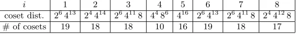
The algorithm was applied to the vector setsTi defined by DES S-boxesSi. Let the sets of cosets Ui be produced. The results are summarised in Table 4, where 2a4b8c meansUi containsacosets of size 2,bcosets of size 4 andccosets of size 8. The distribution is uneven. For instance, S4 admits exceptionally

Table 4.Coset distribution for S-boxes

i 1 2 3 4 5 6 7 8

coset dist. 26₄13 ₂4₄14 ₂6₄11_{8 4}4₈6 ₄16 ₂6₄13 ₂6₄11_{8 2}4₄12₈

# of cosets 19 18 18 10 16 19 18 17

many cosets of size 8. Disjoint sub-cosets which coverTifor eachi= 1, . . . ,8 are listed in Appendix 2, where strings (25) have integer number representation

u529+u428+u327+u226+u125+u024+v323+v222+v12 +v0.

4.1 More Compact DES Equations

Given one plaintext/ciphertext pair one constructs a system of equations in the key bits by introducing new variables after each S-box application, 128 equations for 16-round DES. By specifyingSi,

¯

Xji⊕Kji

P−1_(X

j−1i⊕Xj−2i) =

0 . . . 63

Si(0). . . Si(63)

, (26)

with 64 right hand sides, 10-bit vectorsTiwritten column-wise. Here ¯XjiandKji are 6-bit sub-blocks of ¯Xj and Kj respectively. To find the key such equations are solved. That may be done with methods introduced in [10], see also [9]. The complexity heavily depends on the number of right hand sides.

We get a more compact representation, that is with lower number of sides. We use the previous section notation. LetUi containrcosets. Sox∈Ti if and only ifxis a solution to exactly one of the linear equation systems

We cover the set of right hand side columns in (26) with sub-cosets fromUi and get (26) is equivalent to

_¯

Xji⊕Kji

P−1_(X

j−1i⊕Xj−2i)

Ak=bk, k= 1, . . . , r (27)

in sense that an assignment to the variables is a solution to (26) if and only if it is a solution to one of (27). The number of subsystems(also called sides) in (27), denoted byr, is between 10 and 19 depending on the S-box. For instance, in case ofS4 the equation (27) has only 10 subsystems, while (26) has 64. Such

reduction generally allows a faster solution, see [11].

5

Conclusion and Open Problems

In the present paper new statistical and algebraic properties of the DES encryp-tion were found. They may have cryptanalytic implicaencryp-tions upon resolving the following theoretical questions.

The first problem is within the statistical cryptanalysis. Let the cipher key space be split into n classes K1, . . . , Kn. Each class defines a multinomial dis-tribution on some ≥2 outcomes, defined by plaintext and ciphertext bits. Let

P1, . . . , Pn be all such distributions computed a priori. Let ν(k) denote a vec-tor of observations on above outcomes for an unknown cipher key k. It is well known that the problem “decide k ∈ Ki” may be solved with maximum like-lihood method as in [5]. For the classification of several observation vectors

ν(k1), . . . , ν(ks) the same method is applied.

Open problem is to improve the method (reduce error probabilities) given the vectorsP1, . . . , Pn are linearly dependent. That would improve Davies-Murphy type attacks against 16-round DES as for 660 different distributions (72 for (S4, S5, S6)) only≤48 (13 for (S4, S5, S6)) are linearly independent.

The second problem is related to algebraic attacks against ciphers. A new type time-memory trade-off for AES and DES was observed in [9,10]. Letm be the cipher key size. Let ≤ 2l _{right hand sides be allowed in the combinations} by Gluing of the MRHS equations [9,10] during solution. Gluing means writ-ing several equations as one equation of the same type as (26). Then guesswrit-ing

≤ m−l key-bits is enough before the system of equations is solved by finding and removing contradictory right-hand sides in pairwise agreeing of the current equations. The overall time complexity is at least 2m−l×2l= 2moperations as for each guess one needs to run over the right hand sides of at least one of the equations. However coset representation allows reducing the number of sides by writing them as (27). In case of DES the equation (26) fori= 4 is written with only 10 sides instead of 64. For AES instead of 256 right hand sides one can do 64 for each of the equations, see [11]. The combination of two equations (26) with Gluing has≤212 _{right hand sides. With coset representation the number}

of sides is at most 192 _{(at most 100 for the combination of two equations from} S4). Open problem is to reduce the time complexity of the above trade-off by

Acknowledgement

Stian Fauskanger is supported by the COINS Research School of Computer and Information Security.

References

1. Barker, W.C., Barker, E.B.: SP 800-67 Rev. 1. Recommendation for the Triple Data Encryption Algorithm (TDEA) Block Cipher (Jan 2012)

2. Biham, E., Biryukov, A.: An improvement of Davies’ attack on DES. Journal of Cryptology 10(3), 195–205 (Jun 1997)

3. Biham, E., Shamir, A.: Differential Cryptanalysis of the Full 16-round DES. Ad-vances in Cryptology CRYPTO 92 740, 487–496 (May 1993)

4. Courtois, N.T., Bard, G.V.: Algebraic Cryptanalysis of the Data Encryption Stan-dard. Cryptography and Coding 4887, 152–169 (2007)

5. Davies, D., Murphy, S.: Pairs and triplets of DES S-boxes. Journal of Cryptology 8(1) (1995)

6. Kholosha, A.: Personal conversation with I. Semaev (Sep 2014)

7. Kunz-Jacques, S., Muller, F.: New Improvements of Davies-Murphy Cryptanalysis. Advances in Cryptology - ASIACRYPT 2005 3788, 425–442 (2005)

8. Matsui, M.: Linear Cryptanalysis Method for DES Cipher. Advances in Cryptology EUROCRYPT 93 765, 386–397 (Jul 1994)

9. Raddum, H.v.: MRHS Equation Systems. Selected Areas in Cryptography 4876, 232–245 (2007)

10. Raddum, H.v., Semaev, I.: Solving Multiple Right Hand Sides linear equations. Designs, Codes and Cryptography 49(1), 147–160 (Mar 2008)

11. Semaev, I., Mikuˇs, M.: Methods to solve algebraic equations in cryptanalysis. Tatra Mountains Mathematical Publications 45(1), 107–136 (Jan 2010)

12. Shamir, A.: On the Security of DES. Advances in Cryptology CRYPTO 85 Pro-ceedings 218, 280–281 (Dec 1986)

6

Appendix 1 - S

Right, Left and LR Distribution

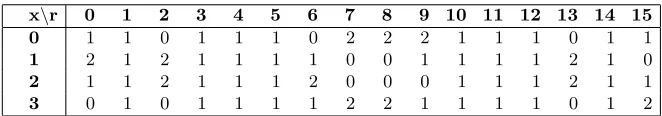
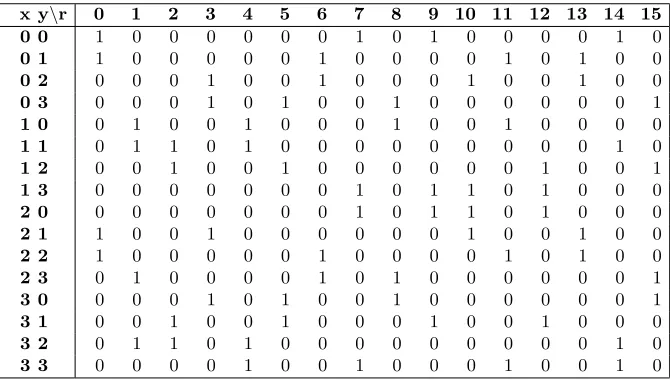
Section 2.1 define the right, left and LR distribution. Tables 5, 6 and 7 show the distributions for S-box 4.

Table 5.Right hand side distribution of S-box 4 (each entry = 26_×p(4) x,r)

x\r 0 1 2 3 4 5 6 7 8 9 10 11 12 13 14 15

0 1 1 0 1 1 1 0 2 2 2 1 1 1 0 1 1

1 2 1 2 1 1 1 1 0 0 1 1 1 1 2 1 0

2 1 1 2 1 1 1 2 0 0 0 1 1 1 2 1 1

Table 6.Left hand side distribution of S-box 4 (each entry = 26×qx,r(4))

x\r 0 1 2 3 4 5 6 7 8 9 10 11 12 13 14 15

0 2 0 0 2 0 1 2 1 1 1 1 1 0 2 1 1

1 0 2 2 0 2 1 0 1 1 1 1 1 2 0 1 1

2 2 1 0 1 0 0 2 1 1 1 2 1 1 2 0 1

3 0 1 2 1 2 2 0 1 1 1 0 1 1 0 2 1

Table 7.LR distribution of S-box 4 (each entry = 26_×Q(4) x,y,r)

x y\r 0 1 2 3 4 5 6 7 8 9 10 11 12 13 14 15

0 0 1 0 0 0 0 0 0 1 0 1 0 0 0 0 1 0

0 1 1 0 0 0 0 0 1 0 0 0 0 1 0 1 0 0

0 2 0 0 0 1 0 0 1 0 0 0 1 0 0 1 0 0

0 3 0 0 0 1 0 1 0 0 1 0 0 0 0 0 0 1

1 0 0 1 0 0 1 0 0 0 1 0 0 1 0 0 0 0

1 1 0 1 1 0 1 0 0 0 0 0 0 0 0 0 1 0

1 2 0 0 1 0 0 1 0 0 0 0 0 0 1 0 0 1

1 3 0 0 0 0 0 0 0 1 0 1 1 0 1 0 0 0

2 0 0 0 0 0 0 0 0 1 0 1 1 0 1 0 0 0

2 1 1 0 0 1 0 0 0 0 0 0 1 0 0 1 0 0

2 2 1 0 0 0 0 0 1 0 0 0 0 1 0 1 0 0

2 3 0 1 0 0 0 0 1 0 1 0 0 0 0 0 0 1

3 0 0 0 0 1 0 1 0 0 1 0 0 0 0 0 0 1

3 1 0 0 1 0 0 1 0 0 0 1 0 0 1 0 0 0

3 2 0 1 1 0 1 0 0 0 0 0 0 0 0 0 1 0

7

Appendix 2 - Disjoint Sub-cosets for DES S-boxes

U1={{516,626},{678,697},{812,827},{841,894},{899,922},{944,992},

{14,36,326,364},{16,87,175,232},{63,77,572,590},{97,130,545,706}, {116,158,298,448},{178,221,938,965},{203,241,721,747},

{259,282,653,660},{310,379,437,504},{348,389,783,982}, {409,425,600,616},{467,487,851,871},{543,759,789,1021}},

U2={{365,490},{855,870},{892,912},{949,1007},{15,19,33,61},

{72,84,962,990},{110,119,134,159},{171,178,416,441}, {195,216,676,703},{228,254,396,406},{265,295,475,501}, {284,304,583,619},{322,337,737,754},{378,453,822,905}, {512,602,931,1017},{541,558,795,808},{568,625,773,844}, {650,659,717,724}},

U3={{341,497},{605,624},{648,697},{707,759},{876,974},{978,1020},

{10,29,110,121},{32,134,301,395},{73,80,207,214}, {163,229,312,382},{180,250,662,728},{257,359,420,450}, {274,412,779,901},{443,479,525,617},{529,687,788,938}, {550,570,834,862},{801,883,949,999},

{55,147,332,488,580,736,831,923}},

U4={{45,56,290,311},{395,401,452,478},{711,733,968,978},

{801,820,878,891},{7,29,328,338,683,689,996,1022},

{78,91,257,276,749,760,930,951},{99,117,428,442,652,666,835,853}, {128,150,495,505,608,630,783,793},

{166,191,201,208,550,575,585,592}, {234,243,357,380,522,531,901,924}},

U5={{2,30,323,351},{44,59,230,241},{68,82,203,221},{97,124,170,183},

U6={{467,504},{591,693},{735,762},{795,836},{887,897},{918,971},

{12,26,256,278},{33,63,74,84},{111,114,232,245}, {137,151,162,188},{198,301,563,984},{217,305,642,874}, {323,349,398,400},{356,423,830,1021},{382,443,521,716}, {453,491,594,636},{532,613,800,849},{558,665,775,944}, {680,739,941,998}},

U7={{402,481},{534,587},{621,632},{848,872},{926,946},{979,1020},

{29,43,143,185},{48,66,426,472},{91,110,329,380}, {148,160,730,750},{200,237,513,548},{209,250,969,994}, {259,286,652,657},{300,341,447,454},{307,359,675,759}, {571,605,793,895},{778,815,896,933},

{4,119,389,502,692,711,821,838}},

U8={{446,498},{519,684},{806,911},{949,1019},{13,17,100,120},

{34,63,649,660},{72,134,297,487},{154,179,857,880}, {175,203,266,366},{215,244,530,561},{309,323,828,842}, {342,379,965,1000},{389,400,460,473},{555,765,768,982}, {580,698,877,915},{609,631,718,728},