Progressive lattice sieving

Progressive lattice sieving

Thijs Laarhoven1 _{and Artur Mariano}2 1

Eindhoven University of Technology, Eindhoven, The Netherlands [email protected]

2

University of Coimbra, Coimbra, Portugal [email protected]

Abstract. Most algorithms for hard lattice problems are based on the principle of rank reduction: to solve a problem in ad-dimensional lattice, one first solves one or more problem instances in a sublattice of rankd−1, and then uses this information to find a solution to the original problem. Existing lattice sieving methods, however, tackle lattice problems such as the shortest vector problem (SVP) directly, and work with the full-rank lattice from the start. Lattice sieving further seems to benefit less from starting with reduced bases than other methods, and finding an approximate solution almost takes as long as finding an exact solution. These properties currently set sieving apart from other methods. In this work we consider a progressive approach to lattice sieving, where we gradually introduce new basis vectors only when the sieve has sta-bilized on the previous basis vectors. This leads to improved (heuristic) guarantees on finding approximate shortest vectors, a bigger practical impact of the quality of the basis on the run-time, better memory man-agement, a smoother and more predictable behavior of the algorithm, and significantly faster convergence – compared to traditional approaches, we save between a factor 20 to 40 in the time complexity for SVP.

Keywords: lattice-based cryptography, lattice sieving, shortest vector problem (SVP), nearest neighbor searching

1

Introduction

Finding short lattice vectors. A central hard problem in the study of lattices is the shortest vector problem (SVP): given a latticeL ={Pd

i=1cibi :ci ∈Z} ⊂ Rd, find a non-zero lattice vectorsof minimum norm, i.e. finds∈ Lsatisfying

Exact SVP algorithms. There are currently two classes of algorithms for ex-act SVP: algorithms requiring superexponential time 2ω(d) _{in the lattice} di-mension d, using a negligible amount of memory (such as enumeration [Kan83, FP85, SE94, GNR10, AN17]), and algorithms requiring single exponential time and space 2Θ(d) _{(such as lattice sieving [AKS01, HPS11] and Voronoi cell} ap-proaches [SFS09, MV10a, Laa16]). Although the latter methods have clear draw-backs due to the large memory requirement, these algorithms will inevitably sur-pass the former algorithms in terms of the time complexity in high dimensions. Conservative estimates of the (post-quantum) hardness of SVP are therefore often based on the state-of-the-art asymptotics for the best (quantum) lattice sieving algorithms [ADPS16, DLL+18, BDK+18].

Lattice sieving. Lattice sieving was introduced in 2001 by Ajtai–Kumar–Siva-kumar [AKS01], and was only made somewhat practical less than 10 years ago with fast heuristics [NV08,MV10b]. Recent years have seen further developments in decreasing the asymptotic time complexity of sieving at the cost of using more space [WLTB11, ZPH13, BGJ14, Laa15, BGJ15, LdW15, BL16, BDGL16], while tradeoffs in the reverse direction have also been studied recently to reduce the large memory requirement [BLS16, HK17, HKL18]. Various efforts have further been made to make these algorithms competitive in high-performance computing environments [Sch11,MS11,Sch13,FBB+_{14,MTB14,MODB14,IKMT14,MLB15,} BNvdP16, MB16, MLB17, YKYC17, Duc18]. The theoretically fastest method in high dimensions is currently the LDSieve, with asymptotic time and space com-plexities 20.29d+o(d) [BDGL16], while in practice the GaussSieve and HashSieve appear to be the most practical in high dimensions [MB16, MLB17, YKYC17].

Differences with other approaches. Existing lattice sieving methods are fun-damentally different from other SVP approaches in several ways. Whereas for instance enumeration and Voronoi cell-based methods use a rank reduction step to reduce a d-dimensional problem to problems in lattices of rankd−1, lattice sieving never considers other lattices than the full-rank one. And unlike other methods, lattice sieving (i) does not appear to benefit greatly from being given better lattice bases as input (i.e. BKZ-reduced bases with larger block sizes), and (ii) does not appear to be much faster when an approximate solution suffices – often the algorithm only starts to find shorter vectors after the algorithm is al-ready 80% finished with finding an exact solution. All these properties currently set sieving apart from other methods, and so one might ask whether lattice siev-ing can be adjusted and perhaps improved by applysiev-ing similar rank-reduction techniques, so that sieving also obtains these “natural” properties of finding short vectors faster, and performing better when given more reduced bases.

1.1 Contributions

lattice sieving uses a bottom-up approach, initially starting with sieving in a low-rank sublattice of the input lattice. Then, when this subspace of the original space has been saturated with vectors from this sublattice, new basis vectors are introduced to find shorter lattice vectors in sublattices of higher rank, until ultimately the algorithm reaches the full-rank lattice and attempts to find short vectors in the original lattice. Using this rank reduction approach, progressive sieving offers various benefits over standard sieving techniques, which we list below. These are mostly independent of the exact underlying sieve used (e.g. the GaussSieve [MV10b], HashSieve [Laa15], or LDSieve [BDGL16]), although in some cases the improvements are bigger than in other cases.

Faster convergence: Overall, progressive sieving finds shortest vectors in lat-tices much faster than using current methods, with speedups as large as a factor 40 in dimension 70. Tables 1–2 illustrate improvements for 70-dimensional lattices for the GaussSieve and HashSieve, and Figure 1 shows the improvements for various dimensions using progressive sieving.

Better memory usage: Working on low-rank lattices requires fewer vectors to make progress, allowing one to do a large part of the algorithm using much less memory than current approaches. Experiments further show progres-sive sieving uses slightly less memory overall (Figure 2b). This is especially relevant as the main bottleneck in sieving is hitting the memory wall [MB16]. Heuristic guarantees for approximate SVP: Using the Geometric Series Assumption, progressive sieving heuristically finds approximate solutions faster than the full solution, unlike other approaches which commonly re-quire a large number of vectors and reductions to make any progress at all.3 Larger impact of reduced bases: The more reduced the input basis is, the faster shorter lattice vectors are found, which contributes to a faster overall running time. Similar to pruning in enumeration, this further opens up some new directions for potential improvements (see Section 5.2).

Better predictability: As illustrated in the experimental profiles (Figures 2– 3), various aspects of sieving are easier to predict and easier to explain theoretically with progressive sieving, which may lead to more accurate pre-dictions when extrapolating to higher dimensions.

Less resource contention: Vectors in the sieved list are only modified sporad-ically. Instead of using the lock-free mechanism of [MB16, MLB17], to avoid collisions between different nodes, we may therefore be able to construct parallel implementations with lower-overhead incurring mechanisms.

Outline. The remainder of this paper is organized as follows. In Section 2, we in-troduce notation and related work on lattice sieving. Section 3 describes progres-sive sieving, and an experimental comparison with previous approaches is given in Section 4. Section 5 discusses various aspects of these different approaches to sieving, and Section 6 concludes with open problems for future work.

3

Exact SVP ←−GaussSieve −→ ←−HashSieve −→

LLL BKZ-10 BKZ-30 LLL BKZ-10 BKZ-30

Standard sieving 19100 18100 16500 3300 3050 2900

Progressive sieving 595 440 390 165 125 115

Speedup factor 32× 41× 42× 20× 24× 25×

Table 1.Running times (in seconds) for solving exact SVP on 70-dimensional lattices from the SVP challenge [SVP18], using the baseline GaussSieve algorithm [MV10b] and the near-neighbor-based HashSieve extension of the GaussSieve [Laa15]. The lattice bases are pre-reduced with either LLL or BKZ with blocksize 10 or 30, where we used fplll[fplll18] to perform the basis reduction. The timings above are based only on the sieving step, and do not include the time for the basis reduction step.

★ ★ ★ ★ ★ ★ ★ ★ ★ ★ ★ ● ● ● ● ● ● ● ● ● ★ ★ ★ ★ ★ ★ ● ● ● ● ● ● ● ★ GaussSieve ● HashSieve ★ ProGaussSieve ● ProHashSieve

40 50 60 70 80

0.1 1 10 100 1000 104 105 Dimension d Time ( seconds )

2

d-22

2

2

d-25

2

d-22

Fig. 1.Time complexities for solving exact SVP on BKZ-10 reduced bases for the SVP challenge lattices, using standard lattice sieving approaches (GaussSieve and Hash-Sieve) and progressive sieving modifications of these algorithms (ProGaussSieve and ProHashSieve). The formulas written in the figure denote the least-squares fits of the four data sets up to two significant digits.

2

Preliminaries

Given a setB={b1, . . . ,bm} ⊂Rdofmindependentd-dimensional vectors, we denote the (rank-m) lattice spanned byBbyL(B) ={Pm

i=1cibi :ci ∈Z}. With abuse of notation, we sometimes write L=L(B) when the basisBis implicit. For k ≤m, we write Lk =Lk(B) for the sublattice {P

k

i=1cibi : ci ∈Z} ⊆ L spanned by the firstk basis vectors of B. For simplicity, we commonly assume that the original problem concerns a lattice problem in a lattice of full rank (m = d); however, using rank reduction we sometimes consider problems in sublattices as well. We denote by Vol(L) =pdet(BT_{B) the volume of a lattice}

L, and by Vol(A) the volume of a setA ⊂Rd.

2.1 Heuristic assumptions

To analyze lattice algorithms, various heuristic assumptions are commonly used. These are not proven and may well be false for certain extreme lattices/bases, but commonly hold forrandom lattices encountered in cryptography. Analyzing algorithms under these (average-case) assumptions therefore commonly leads to more accurate security assessments than analyses based on provable (worst-case) bounds, which are commonly not tight for random lattices.

TheGaussian heuristic states that, given a subset A ⊂Rd, the number of lattice points in A is roughly|A ∩ L| ≈Vol(A)/Vol(L). As a consequence, we expect a ball of radius r around a random point in space to contain a lattice point iffr≥r0∼p

d/(2πe), and heuristically we expectλ1(L)≈p

d/(2πe). TheGeometric Series Assumption (GSA)states that, after performing BKZ reduction [Sch87] with block-sizeβon a full-rank lattice basis, the Gram-Schmidt orthogonalizationb∗₁. . .b∗_dof the output basis satisfieskb_i∗k ≈δd−2i+1·Vol(L)1/d for all i. Here δ =δ(β) determines the quality of the basis; the smaller δ, the more orthogonal the basis and the shorterb1. Note thatQ

d i=1kb

∗

ik= Vol(L).

2.2 Lattice sieving algorithms

Algorithm 1ThestandardGaussSieve algorithm –GaussSieve 1: Initialize an empty listL← ∅and an empty stackS← ∅

2: Initializecollisions←0 3: while true do

4: Get a vectorvfrom the stackS or sample a new one fromL(b1, . . . ,bd) 5: Reducevwith allw∈L // this naively takes O(|L|) time 6: Reduce allw∈Lwithv // NNS can speed up these searches 7: Move reduced vectorsw∈L from the listLto the stackS

8: if vhas not changedthen 9: Addvto the listL 10: else

11: if v6= 0then

12: Addvto the stackS 13: else

14: _collisions++

15: if collisions= 100then // a target norm may be used instead 16: returnargmin_v∈Lkvk // the shortest vector found so far

The GaussSieve and ListSieve. In 2010, Micciancio–Voulgaris [MV10b] intro-duced two new (heuristic) lattice sieving algorithms, which unlike the Nguyen– Vidick sieve both start from an empty list L, and gradually grow this list by adding more (short) lattice vectors to the list, until this list contains a solution. In the ListSieve, before adding a randomly sampled lattice vector v to the list, the vector is reduced with all list vectorsw∈Lby checking whether either of the sum/difference vectors v±w are shorter than v – if so, v is replaced by this shorter vector. Once v has been reduced with all list vectors, and no pairwise sums/differences with list vectors lead to shorter vectors anymore,v is added to the list. This process is repeated untilLcontains a shortest vector.

In theGaussSievethis process is essentially the same, except that list vectors w ∈ Lare also reduced with newly sampled vectors v, before adding v to the list; in contrast, in the ListSieve vectors which have been added to the list L are never modified again. Algorithm 1 describes the GaussSieve, while removing Lines 6–7 leads to the ListSieve algorithm.

Extensions and variants. Over the last few years, various extensions and variants of these heuristic sieving algorithms have been studied, to make them even more efficient in practice. High-dimensional nearest neighbor search algorithms have been used to obtain speed-ups in the searches in Lines 5–6 of Algorithm 1, which naively take time O(|L|) but can be done in sublinear timeO(|L|ρ_{) with ρ <1} with more advanced methods of indexing and querying the listL[Laa15,LdW15, BGJ15, BL16, BDGL16]. Recent work on tuple sieving [BLS16, HK17, HKL18] focused on reducing the memory of lattice sieving, by considering a larger number of vectors w1, . . . ,wk ∈ L from the list to form short combinations v±w1±

3

Progressive lattice sieving

When given a (full-rank)d-dimensional lattice basis, standard sieving approaches attempt to saturate this entired-dimensional space from the start, always work-ing with vectors from the full-dimensional space. With pairwise reductions be-tween lattice vectors, one needs roughly 20.21d+o(d)vectors to saturate this space and make significant progress in obtaining shorter vectors. This means that also approximate shorter vectors are not found until the list size approaches 20.21d+o(d)_{, which means a lot of effort is spent even before any progress is made} at all. Naively this means the time complexity to find any shorter vectors at all is at least 20.42d+o(d) _{(or 2}0.29d+o(d)_{using near neighbor techniques [BDGL16]).} Using BKZ, finding approximate shortest vectors does not necessarily require the same amount of effort as finding exact solutions. More specifically, BKZ only solves SVP instances in lower-dimensional lattices, thereby finding short lattice vectors in (projected) sublattices sooner. The idea of progressive lattice sieving is similar: by first considering low-dimensional sublattices of the full lattice, which already contain many short lattice vectors, we will find approximate solutions faster, which will eventually contribute to finding exact solutions faster as well.

The GaussSieve. Applying progressive sieving to the GaussSieve means mak-ing the followmak-ing modifications. First, we start with a sublattice of the original lattice, spanned by the first few basis vectors. We then run a sieve on this sub-lattice, until we reach the stopping criterion (e.g. a certain number of collisions). We then add a new basis vector to the search space, and continue sieving in this sublattice of slightly higher rank. We repeat this procedure until we reach the complete lattice, where we expect to find an exact solution to SVP. The result of applying progressive sieving to the GaussSieve is sketched in Algorithm 2, where the main modifications are (1) vectors are sampled from sublattices, and (2) the rank counter is increased and the collision counter is reset when we reach 100 collisions. For simplicity we start with a sublattice of rank 10 – everything below rank 30 or 40 generally finishes within a second anyway, so setting the initial rank to any rank below 40 will lead to similar results in higher dimensions.

Algorithm 2TheprogressiveGaussSieve algorithm –ProGaussSieve

1: Initialize an empty listL← ∅and an empty stackS← ∅ 2: Initializecollisions←0,rank←min{10, d}

3: while true do

4: Get a vectorvfrom the stackS or sample a new one fromL(b1, . . . ,brank) 5: Reducevwith allw∈L // this naively takes O(|L|) time 6: Reduce allw∈Lwithv // NNS can speed up these searches 7: Move reduced vectorsw∈L from the listLto the stackS

8: if vhas not changedthen 9: Addvto the listL 10: else

11: if v6= 0then

12: Addvto the stackS 13: else

14: _collisions++

15: if collisions= 100then 16: if _rank=dthen

17: returnargminv∈Lkvk// the shortest vector found so far

18: else

19: _rank++ // continue with the next sublattice

20: collisions←0 // reset the collisions counter

4

Experiments

Heuristically, sieving naively requires a search over all pairs of vectors in the list (when not using near neighbor techniques), leading to a quadratic time com-plexity in the list size. With progressive sieving, these arguments still hold, and so the asymptotic improvement of progressive sieving will not be visible in the leading time/memory exponents. Experimentally however there are rather large hidden order terms, and these may become smaller with progressive sieving. To get an insight into this improvement, we will experimentally evaluate progres-sive sieving and compare it to standard sieving approaches. As a baseline we will use the GaussSieve [MV10b], the baseline sieve without near neighbor searching, and the HashSieve [Laa15], which is perhaps the most practical near neighbor extension of the GaussSieve to date [MLB15, MB16, MLB17]. In Section 5 we will give a more in-depth discussion of various aspects of these results.

4.1 Profiles

To get an idea how progressive sieving differs from classical sieving in practice, Figures 2–3 depict typical profiles of the classical and progressive HashSieve, when solving SVP on 70-dimensional lattices from the SVP challenge [SVP18]. As described in the captions of the figures, the time complexities are significantly better, the list size increases more steadily (and predictably) than in the original HashSieve, approximate solutions are found considerably faster, and vectors in the list are updated much less frequently in progressive sieving.

Note that as in Figure 2c, classical sieving can be viewed as a special case of progressive sieving, with the initial value of rankset tod. Also note that in all figures, the horizontal axis counts the number ofiterations of thewhile-loop of Algorithms 1–2), which translates to actual time complexities as in Figure 2a – this means that e.g. a vector of Euclidean norm 2400 in this 70-dimensional lattice is not found a factor 5×faster (as one might guess from Figure 3a), but close to a factor 5·20≈1000×faster (taking into account Figure 2a).

4.2 Results

To get reliable complexity estimates for arbitrary dimensions, we ran several ex-periments of both standard and progressive sieving on lattices of dimensions 40 to 80, the results of which are displayed in Figure 1. These results clearly show a large decrease in the time complexities for sieving in arbitrary dimensions, both for the classical GaussSieve and the near-neighbor-optimized HashSieve algo-rithm [Laa15]. For both algoalgo-rithms the improvement is more than a factor 20×

for all tested dimensions, showing that the improvement of progressive sieving can indeed be combined with near neighbor techniques.

Focusing only on 70-dimensional lattices, we also ran experiments with dif-ferent quality bases, to see how the basis reduction affects the performance of (progressive) sieving. The results in Table 1 are based on at least 10 experiments each on randomized lattice bases (where only the experiments that took several hours are based on just 10 runs). As can be seen in the table, progressive siev-ing benefits more from reduced bases, with the speedup factor increassiev-ing as the quality of the basis improves. We further observe that the speedup factor for the HashSieve is slightly smaller than for the GaussSieve, which can be explained by the HashSieve spending most of its time working with the near neighbor data structure – costs which are not affected by progressive sieving.

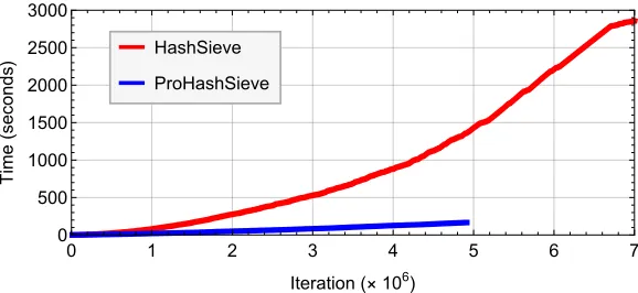
HashSieve

ProHashSieve

0 1 2 3 4 5 6 7

0 500 1000 1500 2000 2500 3000

Iteration(×106₎

Time

(

seconds

)

(a)Time complexities. Iterations (Line 3) take significantly less time in the ProHashSieve, leading to finding short lattice vectors much faster.

HashSieve

ProHashSieve

0 1 2 3 4 5 6 7

0 20 40 60 80

Iteration(×106₎

List

size

(×

1000

)

(b)List sizes.Whereas the list size behaves rather erratically in the orig-inal HashSieve, the ProHashSieve shows a much more steady behavior.

HashSieve

ProHashSieve

0 1 2 3 4 5 6 7

30 40 50 60 70

Iteration(×106₎

Lattice

rank

(c) Lattice rank. For the ProHashSieve, the rank of the sublattice (roughly) follows a square-root law, with more time spent on higher ranks.

HashSieve

ProHashSieve

0 1 2 3 4 5 6 7

2000 2200 2400 2600 2800 3000

Iteration(×106₎

Norm

of

shortest

vector

(a)Norm of the shortest vector.The dashed black curve shows the theoretical prediction for the ProHashSieve based on the GSA and rank.

HS: Reducing v with L HS: Reducing L with v PHS: Reducing v with L PHS: Reducing L with v

0 1 2 3 4 5 6 7

0 1 2 3 4 5 6 7

Iteration(×106₎

Reductions

(×

10

6 )

(b)Reductions (×106_{).Progressive sieving rarely sees reductions of the} list with new vectors, making the GaussSieve similar to the ListSieve.

HS: Comparisons HS: Hashes PHS: Comparisons PHS: Hashes

0 1 2 3 4 5 6 7

0 5 10 15 20 25 30 35

Iteration(×106)

Operations

(×

10

9 )

(c)Operations (×109).Both algorithms roughly have the same ratio of hashing operations (finding near neighbors) and vector comparisons.

Approximate SVP ←−GaussSieve −→ ←−HashSieve −→

(γ=1.1) LLL BKZ-10 BKZ-30 LLL BKZ-10 BKZ-30

Standard sieving 18500 17200 15600 3180 2960 2700

Progressive sieving 120 40 3 65 20 2

Speedup factor 150× 400× 5000× 50× 150× 1000×

Table 2.Running times (in seconds) for solving approximate SVP with approximation factorγ= 1.1 on 70-dimensional lattice bases from the SVP challenge [SVP18]. When the bases are sufficiently well-reduced, low-rank sublattices already contain very short lattice vectors, leading to substantially faster convergence for progressive sieving.

5

Discussion

In this section we will briefly discuss different aspects of lattice sieving, and how various design choices affect the performance of (progressive) sieving in practice.

5.1 Approximate SVP

As shown in Table 2, progressive sieving benefits greatly from being given a relaxed termination condition, in the sense that an approximate solution to SVP suffices. To quantify where this improvement comes from, recall that by the Geometric Series Assumption (GSA), BKZ gives us a reduced lattice basis

{b1, . . . ,bd} where the Gram-Schmidt orthogonalization vectors satisfy kb∗ik ≈ δd−2i+1 _·Vol(L)1/d _{for all i = 1, . . . , d. As a result, the first k basis vectors} together form a rank-k sublatticeLk =L(b1, . . . ,bk)⊂ Lof volume:

Vol(Lk) = k Y

i=1

kb∗_ik= Vol(L)k/d·δPki=1(d−2i+1)= Vol(L)k/d·δk(d−k) (1)

By the Gaussian heuristic we haveλ1(L)≈Vol(L)1/d/

√

2eπd, and therefore the shortest vector in this rank-ksublatticeLk has relative norm:

λ1(Lk)≈

Vol(Lk)1/k

√

2eπk =

δd−kVol(L)1/d

√

2eπk ≈δ d−k

r d

k ·λ1(L) (2) To obtain a solution toγ-SVP, i.e. approximate SVP with approximation factor γ, we needδd−kp

d/k≈γ. Depending on the basis quality δ, dimensiond, and approximation factor γ, this tells us how many dimensions we can essentially “skip” at the end when looking for approximate solutions: already at rankk, we will then expect to find a vector of sufficiently short length.

k is required to find an approximate solution in a suitable sublattice, and then (b) simply running sieving on such a sublattice until an approximate solution has been found. Even in that case however, progressive sieving has the benefits of not requiring an a priori choice of k(it automatically finds the right rank k required to find a sufficiently short vector), and having a faster convergence for exact SVP in such sublattices as well (as sketched in Table 1).

5.2 Effects of basis reduction

The experiments in Section 4 further suggest that progressive sieving benefits more from being given a more reduced basis than classical sieving approaches. To explain this, we observe that there are two sides to having better bases, and previous sieving approaches only benefited from one of these advantages.

Standard sieving. When given a better basis, classical sieving methods will be able to sample shorter lattice vectors in Line 4 more easily. Being able to sample shorter vectors means that vectors will need to be reduced less frequently before “stabilizing” in the list, thus reducing the overall cost of the algorithm as for each vector, we might save some searches and reductions.

Progressive sieving. Besides the benefit stated above, which also holds for progressive sieving, there is a second advantage to being given a nice lattice basis. This is closely related to the heuristic analysis for approximate SVP above, as having a reduced basis means thatδis smaller and therefore low-rank sublattices will already contain shorter lattice vectors. And being able to find very short lattice vectors early in low ranks, which will then be contained in the listLwhen moving to higher-rank sublattices, means that reductions will proceed faster in those higher ranks as well.

Formally, letSd−1_={x∈

Rd :kxk= 1}denote the unit sphere, and letv∼

Sd−1 _{be sampled uniformly at random from this sphere. Then, using spherical} cap arguments similar to e.g. [BDGL16], one can show that the probability that v can be reduced with a random vectorw ∈ Sd−1 _{(i.e.kv±wk ≤ kvk) is} (3/4)d+o(d)_≈2−0.21d+o(d)_{. However, when the norms of list vectorswdiffer from} 1, so that the norms ofvandware different, this probability changes. Intuitively, for smallkwk →0 the probability of reducingvwithw approaches 1, as either v +w or v−w is likely to be shorter than v. For large kwk → √2kvk the probability of being able to reducev withw approaches 0, and forkwk ≥2kvk

it is even impossible for such a reduction to take place. For arbitraryα∈(0,√2) and randomw∈αSd−1_{, a geometric exercise shows that this probability scales} as (1−α2_/2)d/2+o(d)_{, showing that if list vectorsw ∈L are a factorαshorter} than the sampled vectorsv, the likelihood thatv can be reduced with the list is exponentially larger (inα) than when vectors in the list have equal norm asv.

faster and more easily. Since in classical sieving approaches it takes much longer to find (approximate) short lattice vectors, previous approaches to sieving do not benefit from this accelerated reductions when the list vectors are short. We believe this mostly explains the bigger improvements to progressive sieving when using more reduced bases.

Pruning. Note that when the lattice basis is very reduced, the last coefficients of the shortest lattice vector in terms of these basis vectors are commonly small or zero. If the search space in the last few coefficients is small, one could simply guess or enumerate these potential coefficients, while doing sieving on the first coefficients. This suggests an approach where we only do sieving up to a certain rank, and for the last few basis vectors we use a different procedure of either guessing the coefficients and randomizing/restarting when we fail (similar to pruned enumeration with randomized bases), or using e.g. enumeration or Babai rounding to deal with these latter dimensions. A somewhat similar idea of dealing with these last dimensions faster was analyzed in [Duc18].

5.3 Effects of the sampler

By the sampler, we are referring to the procedure in Line 4 of Algorithms 1– 2 of sampling new lattice vectors, in case the stack is empty: a new vector is sampled from a certain distribution over the lattice, using some efficient sam-pling algorithm. This samsam-pling is often done through a randomized enumeration procedure [Kle00], and the exact specification of this procedure determines how short the sampled lattice vectors will be, how often similar vectors (in particular, the vector0) are sampled, and how long the procedure takes to produce a new sample.

Standard sieving. Choosing the best parameters for the sampler, to get the best performance for sieving, is a rather cumbersome procedure: there are several parameters to tune in the sampler alone, and the best choice varies per dimension and per lattice sieve method (GaussSieve, HashSieve, etc.). Experiments in the past have shown that for previous sieving approaches, this choice of parameters may also greatly influence the practical performance of the algorithm [IKMT14, FBB+14, MLB15, MB16], which makes this aspect of sieving hard to deal with properly – choosing parameters optimally is both difficult and important.

numbers in Tables 1–2 and Figure 1 may not be entirely accurate when using optimized samplers – our numbers are based on a simple, straightforward proof-of-concept implementation of Klein’s sampler, rather than having optimized all aspects of the algorithm (and in particular this sampling routine).4

5.4 Effects of list updates (GaussSieve vs. ListSieve)

As mentioned, the main difference between Micciancio–Voulgaris’ GaussSieve and ListSieve is that in the ListSieve, vectors that are added to the list are never modified again. By “list updates”, we are referring to either making updates to the list vectors as in the GaussSieve, or never updating list vectors as in the ListSieve algorithm.

Standard sieving. In classical sieving approaches, as can for instance be seen in Figure 3b, lattice vectors in the sieved list are quite often reduced and moved back to the stack, after which they are processed again and pushed back to the list. In the ListSieve-variant of such algorithms, where list vectors are never touched again, one would miss all these reductions, leading to a significantly worse performance overall [MODB14]. Although the ListSieve is conceptually slightly simpler, the performance loss would not be worth it to ever consider using the ListSieve instead of the GaussSieve in high-performance environments.

Progressive sieving. For progressive sieving, reductions of list vectors almost never happen, as can also be seen in Figure 3b. Recall that the experiments de-scribed in Figures 2–3 are based on the GaussSieve-based HashSieve, where such list updates are allowed if they produce shorter lattice vectors. For progressive sieving, the execution times of the GaussSieve and ListSieve variants are much closer, which suggests using ListSieve-like sieving may be practical as well. Note that the ListSieve does not save any inner product computations between sam-pled and list vectors, since we already need to compute v·w to see if v can be reduced with w in Line 5 (before reducingw withv in Line 6), and so the performance is still worse when doing the ListSieve instead of the GaussSieve: skipping potential reductions which are “free” is almost never a wise choice.

A potential application of ListSieve-style sieving, knowing that its perfor-mance is closer to the GaussSieve when using progressive sieving, is in parallel implementations. For shared memory systems, current approaches use (proba-ble) lock-free lists [MTB14, MLB15, MLB17], and these lock-free lists may no longer be needed when we know that once a vector is added to the list, it is never updated again and it becomes read-only memory. For distributed-memory implementations [IKMT14, BNvdP16, YKYC17], using a ListSieve as a baseline

4

may also be beneficial in terms of performance and simplicity – synchronization between nodes only has to be done on local sampled vectors, and not on list vectors which are modified by different nodes.

6

Open problems

As we have seen, progressive sieving has a better (experimental) performance than current sieving approaches in many ways, making sieving slightly smoother, more predictable, less dependent on parameter choices for the sampler, and more dependent on the quality of the input basis. Below we state some open problems for future work, related to the ideas presented in this paper.

6.1 BKZ and sieving on sliding windows

A long-standing open problem is to efficiently implement sieving as the SVP sub-routine for BKZ, which now commonly uses enumeration as its SVP subsub-routine. Only recently has sieving become competitive with enumeration, and projects in this direction are likely ongoing. In particular, an open question is whether sieving can be used inside BKZ more efficiently than starting from scratch each time, e.g. by reusing sieved vectors in different, overlapping windows, so that the “set-up” costs of sieving are amortized over all blocks [Duc16].

When running BKZ ond-dimensional bases, there is often a sliding window of kindices i+ 1, . . . , i+k, for which SVP ink dimensions needs to be solved to form a properly reduced basis in this block. Then, when this block has been reduced, the index i is increased by 1, and the same procedure is applied to the window i+ 2, . . . , i+k+ 1. Since there is a large overlap between different windows, a natural question is whether dealing with this new block can be done more efficiently than starting from scratch.

This is somewhat similar to progressive sieving, where as an abstraction we start withkbasis vectorsb1, . . . ,bk, and after reducing this basis (running siev-ing on this block), we switch to the next blockπ1(b2), . . . , π1(bk+1), withπ1(x) being the projection ofxorthogonal tob1, andbk+1being linearly independent of the previous basis vectors. So not only do we add a new basis vector bk+1 to the system as in progressive sieving, we remove the contributions ofb1 to all these vectors, and project everything orthogonal tob1.

Given a sieved list L ⊂ L(b1, . . . ,bk), this transformation to the list L0 ⊂

6.2 Enumeration with sieving

Another long-standing open problem in lattice algorithms is to consider ap-proaches based on enumeration and sieving, and combining the “best of both worlds” to construct even better SVP algorithms. As suggested in [Laa16], one potential such combination would consist of running sieving on a subset of the basis (sayb1, . . . ,bk), and then using the sieved list as an approximate Voronoi cell for faster enumeration. This enumeration procedure would then consist of considering combinations of the vectors bk+1, . . . ,bd as in state-of-the-art enu-meration algorithms, and then using the sieved listL⊂ Lk to see whether those enumerated vectors are close to a vector in the sublattice Lk. If it is close to such a vector, the difference with that vector is likely a short vector in the full lattice. In this case sieving would be used as a batch-CVP/CVPP oracle.

While this idea also works with classical sieving methods, it becomes even more natural with progressive sieving, which already considers increasingly large sublattices to make progress. Modifying progressive sieving to the above appli-cation would simply mean changing the upper bound in Line 16 from the full rankdto some boundd0. Similar ideas of combining sieving on a sublattice with enumerating the “last few dimensions” have been studied in [Duc18], but more work is needed to understand the full potential of such a hybrid approach.

Acknowledgments

The authors thank L´eo Ducas for discussions and comments on this topic, and for sharing an early draft of [Duc18]. The first author is supported by the ERC con-solidator grant 617951. The second author was partially supported by Funda¸c˜ao para a Ciˆencia e a Tecnologia (FCT) and Instituto de Telecomunica¸c˜oes under grant UID/EEA/50008/2013.

References

ADPS16. Erdem Alkim, L´eo Ducas, Thomas P¨oppelmann, and Peter Schwabe. Post-quantum key exchange – a new hope. In USENIX Security Symposium, pages 327–343, 2016.

AKS01. Mikl´os Ajtai, Ravi Kumar, and Dandapani Sivakumar. A sieve algorithm for the shortest lattice vector problem. InSTOC, pages 601–610, 2001. AN17. Yoshinori Aono and Phong Q. Nguyˆen. Random sampling revisited: lattice

enumeration with discrete pruning. InEUROCRYPT, 2017.

BDGL16. Anja Becker, L´eo Ducas, Nicolas Gama, and Thijs Laarhoven. New direc-tions in nearest neighbor searching with applicadirec-tions to lattice sieving. In

SODA, pages 10–24, 2016.

BDK+_{18. Joppe Bos, L´eo Ducas, Eike Kiltz, Tancr`ede Lepoint, Vadim Lyubashevsky,} John M. Schanck, Peter Schwabe, and Damien Stehl´e. CRYSTALS – Kyber: a CCA-secure module-lattice-based KEM. InEuroS&P, 2018.

BGJ15. Anja Becker, Nicolas Gama, and Antoine Joux. Speeding-up lattice siev-ing without increassiev-ing the memory, ussiev-ing sub-quadratic nearest neighbor search. Cryptology ePrint Archive, Report 2015/522, pages 1–14, 2015. BL16. Anja Becker and Thijs Laarhoven. Efficient (ideal) lattice sieving using

cross-polytope LSH. InAFRICACRYPT, pages 3–23, 2016.

BLS16. Shi Bai, Thijs Laarhoven, and Damien Stehl´e. Tuple lattice sieving. In

ANTS, pages 146–162, 2016.

BNvdP16. Joppe W. Bos, Michael Naehrig, and Joop van de Pol. Sieving for shortest vectors in ideal lattices: a practical perspective. International Journal of Applied Cryptography, pages 1–23, 2016.

CN11. Yuanmi Chen and Phong Q. Nguyˆen. BKZ 2.0: Better lattice security estimates. InASIACRYPT, pages 1–20, 2011.

DLL+18. L´eo Ducas, Tancr`ede Lepoint, Vadim Lyubashevsky, Peter Schwabe, Gregor Seiler, and Damien Stehl´e. CRYSTALS – Dilithium: Digital signatures from module lattices. InCHES, 2018.

Duc16. L´eo Ducas. Talk at the HEAT workshop in Paris, France, July 2016. Duc18. L´eo Ducas. Shortest vector from lattice sieving: a few dimensions for free.

InEUROCRYPT, 2018.

FBB+14. Robert Fitzpatrick, Christian Bischof, Johannes Buchmann, ¨Ozg¨ur Dagde-len, Florian G¨opfert, Artur Mariano, and Bo-Yin Yang. Tuning GaussSieve for speed. InLATINCRYPT, pages 288–305, 2014.

FP85. Ulrich Fincke and Michael Pohst. Improved methods for calculating vectors of short length in a lattice.Math. of Comp., 44(170):463–471, 1985. fplll18. The FPLLL development team. fplll, a lattice reduction library. Available

athttps://github.com/fplll/fplll, 2016.

GNR10. Nicolas Gama, Phong Q. Nguyˆen, and Oded Regev. Lattice enumeration using extreme pruning. InEUROCRYPT, pages 257–278, 2010.

HK17. Gottfried Herold and Elena Kirshanova. Improved algorithms for the ap-proximatek-list problem in Euclidean norm. InPKC, pages 327–343, 2017. HKL18. Gottfried Herold, Elena Kirshanova, and Thijs Laarhoven. Speed-ups and

time-memory trade-offs for tuple lattice sieving. InPKC, 2018.

HPS11. Guillaume Hanrot, Xavier Pujol, and Damien Stehl´e. Algorithms for the shortest and closest lattice vector problems. InIWCC, pages 159–190, 2011. IKMT14. Tsukasa Ishiguro, Shinsaku Kiyomoto, Yutaka Miyake, and Tsuyoshi Tak-agi. Parallel Gauss Sieve algorithm: Solving the SVP challenge over a 128-dimensional ideal lattice. InPKC, pages 411–428, 2014.

Kan83. Ravi Kannan. Improved algorithms for integer programming and related lattice problems. InSTOC, pages 193–206, 1983.

Kle00. Philip Klein. Finding the closest lattice vector when it’s unusually close. InSODA, pages 937–941, 2000.

Laa15. Thijs Laarhoven. Sieving for shortest vectors in lattices using angular locality-sensitive hashing. InCRYPTO, pages 3–22, 2015.

Laa16. Thijs Laarhoven. Finding closest lattice vectors using approximate Voronoi cells. Cryptology ePrint Archive, Report 2016/888, 2016.

LdW15. Thijs Laarhoven and Benne de Weger. Faster sieving for shortest lattice vectors using spherical locality-sensitive hashing. InLATINCRYPT, pages 101–118, 2015.

MLB15. Artur Mariano, Thijs Laarhoven, and Christian Bischof. Parallel (probable) lock-free HashSieve: a practical sieving algorithm for the SVP. InICPP, pages 590–599, 2015.

MLB17. Artur Mariano, Thijs Laarhoven, and Christian Bischof. A parallel variant of LDSieve for the SVP on lattices. PDP, 2017.

MLC+17. Artur Mariano, Thijs Laarhoven, F´abio Correia, Manuel Rodrigues, and Gabriel Falcao. A practical view of the state-of-the-art of lattice-based cryptanalysis. IEEE Access, 5:24184–24202, 2017.

MODB14. Artur Mariano, ¨Ozg¨ur Dagdelen, and Christian Bischof. A comprehensive empirical comparison of parallel ListSieve and GaussSieve. In Euro-Par 2014, pages 48–59, 2014.

MS11. Benjamin Milde and Michael Schneider. A parallel implementation of GaussSieve for the shortest vector problem in lattices. InPACT, 2011. MTB14. Artur Mariano, Shahar Timnat, and Christian Bischof. Lock-free

Gauss-Sieve for linear speedups in parallel high performance SVP calculation. In

SBAC-PAD, pages 278–285, 2014.

MV10a. Daniele Micciancio and Panagiotis Voulgaris. A deterministic single ex-ponential time algorithm for most lattice problems based on Voronoi cell computations. InSTOC, pages 351–358, 2010.

MV10b. Daniele Micciancio and Panagiotis Voulgaris. Faster exponential time algo-rithms for the shortest vector problem. InSODA, pages 1468–1480, 2010. NV08. Phong Q. Nguyˆen and Thomas Vidick. Sieve algorithms for the shortest vec-tor problem are practical. Journal of Mathematical Cryptology, 2(2):181– 207, 2008.

Sch87. Claus-Peter Schnorr. A hierarchy of polynomial time lattice basis reduction algorithms. Theoretical Computer Science, 53(2–3):201–224, 1987. Sch11. Michael Schneider. Analysis of Gauss-Sieve for solving the shortest vector

problem in lattices. InWALCOM, pages 89–97, 2011.

Sch13. Michael Schneider. Sieving for short vectors in ideal lattices. In

AFRICACRYPT, pages 375–391, 2013.

SE94. Claus-Peter Schnorr and Martin Euchner. Lattice basis reduction: Im-proved practical algorithms and solving subset sum problems.Mathematical Programming, 66(2–3):181–199, 1994.

SFS09. Naftali Sommer, Meir Feder, and Ofir Shalvi. Finding the closest lat-tice point by iterative slicing. SIAM Journal of Discrete Mathematics, 23(2):715–731, 2009.

SVP18. SVP challenge, 2018.https://latticechallenge.org/svp-challenge/. WLTB11. Xiaoyun Wang, Mingjie Liu, Chengliang Tian, and Jingguo Bi. Improved

Nguyen-Vidick heuristic sieve algorithm for shortest vector problem. In

ASIACCS, pages 1–9, 2011.

YKYC17. Shang-Yi Yang, Po-Chun Kuo, Bo-Yin Yang, and Chen-Mou Cheng. Gauss sieve algorithm on GPUs. InCT-RSA, pages 39–57, 2017.