Colberg, Joerg (1999): Parallel Supercomputer Simulations of Cosmic Evolution. Dissertation, LMU München: Fakultät für Physik

Parallel Supercomputer Simulations

of

Cosmic Evolution

Dissertation der Fakult¨at f¨ur Physik

der

Ludwig–Maximilians–Universit¨at M¨unchen

vorgelegt von

J¨org Colberg

aus Wilhelmshaven

Parallel Supercomputer Simulations

of

Cosmic Evolution

Dissertation der Fakult¨at f¨ur Physik

der

Ludwig–Maximilians–Universit¨at M¨unchen

vorgelegt von

J¨org Colberg

aus Wilhelmshaven

1. Gutachter: Prof. Simon D.M. White

2. Gutachter: Prof. Herbert Wagner

Contents

1. Simulationen der Entstehung von Strukturen im Kosmos 1

1.1. Einleitung . . . 1

1.1.1. Moderne Kosmologie und das Cold Dark Matter–Modell . . . 2

1.2. Die Verteilung der Materie auf großen Skalen . . . 5

1.3. Pekuliargeschwindigkeiten von Galaxienhaufen . . . 6

1.4. Simulationen des Hubble Volumens . . . 8

2. Introduction 15 2.1. Basic Cosmology . . . 17

2.2. The Growth of Perturbations . . . 19

2.3. The Cold Dark Matter Model . . . 21

2.3.1. Introduction . . . 21

2.3.2. Dark Matter . . . 22

2.3.3. Inflation as the Origin of Fluctuations . . . 24

2.3.4. The Fluctuation Spectrum and the Amplitude of Mass Fluctuations . 25 2.3.5. Cold Dark Matter Models . . . 26

3. The Simulation Sets 33 3.1. The Virgo Simulations . . . 33

3.2. The GIF simulations . . . 35

3.3. Visualization Techniques . . . 35

3.3.1. Adaptive Smoothing . . . 35

3.3.2. Cosmology with Pictures . . . 37

4. The Distribution of Mass 43 4.1. Introduction . . . 43

4.2. The Distribution of Mass . . . 44

4.2.1. Introduction . . . 44

4.2.2. Visual Impression . . . 45

4.2.3. Total Mass and Volume Fractions . . . 46

4.2.5. Shape Diagnostics . . . 52

4.3. Conclusions . . . 56

5. Peculiar Velocities of Galaxy Clusters 59 5.1. Introduction . . . 59

5.2. Linear Theory Predictions for the Peculiar Velocities of Peaks . . . 61

5.2.1. The Growth of Peculiar Velocities . . . 61

5.2.2. The Velocities of Peaks . . . 61

5.3. The Simulation Set . . . 63

5.3.1. The Selection of Peaks . . . 64

5.3.2. The Selection of Clusters . . . 65

5.4. Comparison of the Peak Model with Simulations . . . 66

5.4.1. The Cluster-Peak Connection . . . 66

5.4.2. Linear Theory Velocities of Peaks and Clusters . . . 66

5.4.3. The Growth of Cluster Peculiar Velocities . . . 67

5.5. Summary . . . 70

6. Galaxy Clusters in the Hubble Volume Simulations 75 6.1. The Hubble Volume Simulations . . . 75

6.2. Extracting Galaxy Clusters . . . 77

6.3. The Mass Function . . . 78

6.3.1. Massive Objects at High Redshifts . . . 78

6.3.2. The Press–Schechter Mass Function . . . 82

6.4. The Cluster Correlation Function . . . 83

6.4.1. Introduction . . . 83

6.4.2. The Two–point Correlation Function . . . 85

6.4.3. The Mo & White Model . . . 86

6.5. Results from the Hubble Volume . . . 87

6.6. Summary . . . 89

7. Linking Cluster Formation to Large Scale Structure 95 7.1. Introduction . . . 95

7.2. The Formation of Clusters . . . 96

7.2.1. The Simulations . . . 96

7.2.2. The Selection of Clusters . . . 96

7.2.3. Construction of the Formation History . . . 97

7.2.4. Investigating the Formation of the Clusters . . . 97

7.2.5. Connecting Cluster Formation and Large Scale Structure . . . 99

7.2.6. Fraction of Mass in the Peaks . . . 105

8. The N–body Simulations 109

8.1. AP3M . . . 109

8.1.1. Basics . . . 109

8.1.2. The code . . . 111

8.2. Code Development . . . 111

8.2.1. Parallel I/O: Reading in from multiple files . . . 112

9. Summary 125

Chapter

1

Simulationen der Entstehung und

Entwicklung von Strukturen im Kosmos

(Deutsche Zusammenfassung)

Daß die Welt nicht der Inbegriff einer ewigen Vern¨unftigkeit ist, l¨aßt sich endg¨ultig dadurch beweisen, daß jenes St¨uck

Welt, welches wir kennen – ich meine unsre menschliche

Vernunft –, nicht allzu vern¨unftig ist. Und wenn sie nicht allezeit und vollst¨andig weise und rationell ist, so wird es die ¨ubrige Welt auch nicht sein; hier gilt der Schluß a minori ad

maius, a parte ad totum, und zwar mit entscheidender Kraft. Friedrich Nietzsche Menschliches, Allzumenschliches, Bd. 2, 2.2

1.1.

Einleitung

Im Verlaufe der zur¨uckliegenden zwanzig Jahre hat sich die Kosmologie zu einer eigenst¨andigen Wissenschaft entwickelt, die anderen naturwissenschaftlichen Disziplinen in Bezug auf die Pr¨azision von Beobachtungen und theoretischen Vorhersagen in nichts mehr nachsteht. Die Menge an Wissen, die in diesem Zeitraum angeh¨auft werden konnte, l¨aßt einen Vergleich mit der Entwicklung der Quantenmechanik und der nachfolgenden Revolution in der Atomphysik durchaus zu.

Die Kosmologie hat hierbei maßgeblich von den gewaltigen technologischen Entwicklun-gen profitiert. Der COBE–Satellit1zum Beispiel hat die Mikrowellenhintergrundstrahlung mit

einer bis dato unerreichten Pr¨azision vermessen. Dabei zeigte sich, daß diese Strahlung, die die Erde als Nachgl¨uhen des Urknalls erreicht, ein Spektrum hat, das nahezu perfekt dem eines Planck’schen Schwarzen Strahlers entspricht. Zudem muß es im fr¨uhen Universum Dichte– Fluktuationen in der Materie von der Gr¨oßenordnung 10

,5 gegeben haben. Das Hubble–

Space–Teleskop (HST) und neue Teleskope auf der Erde haben es erm ¨oglicht, Galaxien bei einer Rotverschiebung von5zu finden, d.h. zu einer Zeit, als das Universum ein Sechstel seiner

heutigen Gr¨oße hatte. Gleichermaßen zeigte sich in immer deutlicherem Maße, daß ein großer Teil der Materie im Universum in einer Form vorliegt, die sich vollst¨andig von der unterschei-det, wie man sie von der Erde kennt. Diese Dunkle Materie zeigt sich ausschließlich durch den Einfluß ihrer Schwerkraft, indem sie z.B. das Licht von Galaxien, die sich hinter einem Galaxienhaufen befinden, ablenkt und um diesen herum verzerrte Abbilder erzeugt. Diese Liste ist keineswegs vollst¨andig. Alle Theorien der Geburt des Universums und der nachfol-genden Entstehung und Entwicklung von Galaxien und von großr¨aumigen Strukturen m¨ussen ihr Rechnung tragen und Erkl¨arungen und Modelle daf¨ur bieten.

Die neuen Beobachtungsdaten haben Theoretikern abverlangt, bestehende Theorien zu ¨uberpr¨ufen und, wo n¨otig, zu ¨uberarbeiten, insbesondere aber Vorhersagen von gr¨oßerer Pr¨azision zu erarbeiten. Es stellte sich dabei heraus, daß die einfachsten Theorien mit den Beobachtungen nicht zu vereinbaren waren. Allerdings zeigte sich gleichermaßen, daß die notwendigen Korrekturen und Verfeinerungen der Modelle relativ einfach durchzuf¨uhren waren. Computersimulationen haben hierbei eine wichtige Rolle gespielt. Der gewaltige Anstieg der Leistungsf¨ahigkeit moderner Supercomputer ist hierbei nicht der alleinige Grund f¨ur diese Entwicklung. So konnte das Modell, demzufolge die Dunkle Materie ausschließlich aus Neutrinos besteht, mit einer Simulation mit nur 1000 Teilchen ausgeschlossen werden (White et al. 1983). Nichtsdestotrotz waren und sind große Simulationen n¨otig, um hinreichend exakte Vorhersagen zu erzielen. Sehr große Ausschnitte des Universums m¨ussen mit einer ho-hen Massenaufl¨osung simuliert werden, um zuk¨unftige Tests von kosmologischo-hen Modellen zu erm¨oglichen.

Im folgenden Abschnitt werden die zun¨achst die grundlegenden Konzepte moderner Kosmologie und das Cold Dark Matter–Modell motiviert. Abschnitt 1.2 befaßt sich mit der Verteilung der Materie auf großen Skalen. In Abschnitt 1.3 werden die Peku-liargeschwindigkeiten der massereichsten Objekte im Universum (Galaxienhaufen) unter-sucht. Galaxienhaufen stehen auch im Mittelpunkt in Abschnitt 1.4, der die Entstehung und r¨aumliche Verteilung von Galaxienhaufen in den bislang gr¨oßten und umfangreichsten Com-putersimulationen des Universums beschreibt.

1.1.1.

Moderne Kosmologie und das Cold Dark Matter–Modell

Universum gibt. Die Metrik hierf¨ur ist die Friedmann–Robertson–Walker–Metrik

d

s

2

=(

c

d

t

)

2

,

a

2

(

t

) "

d

r

2

1,

kr

2

+

r

2 (d

#

2 +sin 2

_#

d

2 ) #

:

(1.1)

Der sogenannte Expansionsfaktor

a

(

t

) (Dimension: L¨ange) und die Kr¨ummung

k

(dimen-sionslos; nimmt die Werte 1, 0, und -1 an f¨ur positive, keine und negative Kr¨ummung r¨aumlicher Hyperfl¨achen) sind hierbei mithilfe der Einstein’schen Feldgleichungen zu bestim-men. Unter der Annahme von Homogenit¨at und Isotropie lassen sich diese Gleichungen ver-einfacht schreiben als

_

a

2

+

kc

2

a

2 =

8

G

3

;

(1.2)

2 

a

a

+ _

a

2+

kc

2

a

2 = ,8

Gp;

(1.3)

wobei

G

die Gravitationskonstante ist, und

p

und

sind der Druck und die Dichte des Fluids, das sich im Universum befindet. Der Punkt bezeichnet Ableitung nach der Zeit. Es ist ¨ublich in der Kosmologie, folgende Gr¨oßen zu definieren:

H

0 _

a

a

t=t0 (1.4)

c

3

H

20

8

G

(1.5)

0

c (1.6)

Diese sind die sog. Hubble–Konstante zur heutigen Zeit,

H

_{0, die kritische Dichte,}

c, und der Dichteparameter,. Der Kr¨ummungsterm

k

wird dann bestimmt durch

k

=

H

2

0(,1)

:

(1.7)

Das Universum ist nur auf sehr großen Skalen homogen. Das Wachstum von Inhomogenit¨aten aus kleinen Fluktuationen l¨aßt sich in linearer Theorie berechnen. Betrachtet man ein Fluid der Dichte

und Geschwindigkeitvmit

p

=0, das sich in einem Schwerefeld mit dem Potential bewegt, so wird das Fluid beschrieben durch die Kontinuit¨atsgleichung und die Euler– und

Poissongleichungen:

@

@t

+r(

v) = 0

;

(1.8)

@

v

@t

+(vr)v = ,r

;

(1.9)

r

2

= 4

G:

(1.10)

Mit der Annahme eines r¨aumlich variierenden Dichtefeldes

und

1, ergibt sich nach Vernachl¨assigung aller nichtlinearen Terme



+2 _

a

a

_

,4

G

=0

:

(1.12)

Diese Gleichung beschreibt das lineare Wachstum von Strukturen im Universum, die ja, wie durch den COBE–Satelliten best¨atigt, aus sehr kleinen anf¨anglichen Dichteschwankungen re-sultiert sein m¨ussen. F¨ur den einfachen Fall = 1z.B. ergibt sich die anwachsende L¨osung

als2

/

D

(

t

)/

t

2=3

/

a:

(1.13)

D

(

t

)beschreibt hier explizit das Wachstum der Struktur.

t

ist die Zeitvariable. F¨ur

<

1sind

die L¨osungen komplizierter, hier ger¨at der anwachsende Teil der L¨osung in S¨attigung, und die Struktur w¨achst im wesentlichen ab einem bestimmten Zeitpunkt an kaum weiter.

Wie bereits oben angedeutet, gibt es Evidenz, daß ein großer Teil der Materie im Universum in Form von Dunkler Materie vorliegt. Ebenso wurde erw¨ahnt, daß Neutrinos aus theoretischen Erw¨agungen nicht den ¨uberwiegenden Teil dieser Materie stellen k¨onnen. Der Grund hierf¨ur ist, daß sich Neutrinos nach ihrer Entkopplung relativistisch bewegen – sie werden deswegen auch Heiße Dunkle Materie (engl. Hot Dark Matter, HDM) genannt – und so Fluktuationen auf kleinen Skalen auswaschen. Die Struktur, wie sie im Universum beobachtet wird, h¨atte sich nicht bilden k¨onnen. Die Dunkle Materie muß also in einer Form vorliegen, die bei ihrer Entkopplung nichtrelativistisch war. Diese sogenannte Kalte Dunkle Materie (engl. Cold Dark Matter, CDM) konnte bislang noch nicht direkt nachgewiesen werden. Es gibt aber Kandidaten hierf¨ur, Elementarteilchen, wie sie von verschiedenen Erweiterungen des Standardmodells der Elementarteilchenphysik vorhergesagt werden. Als eine der Haupthypothesen dieser Arbeit wird angenommen, daß die Dunkle Materie ausschließlich aus CDM besteht.

Wie sind die Dichteschwankungen im Universum entstanden? Diese Frage wird von einer Theorie beantwortet, die urspr¨unglich viel gewichtigeren Fragen zugewandt war: Warum ist im Universum der Dichteparameter 1? Warum finden sich im Universum nicht die riesige

Anzahl von magnetischen Monopolen, die eigentlich w¨ahrend des Phasen¨ubergangs im fr¨uhen Universum h¨atten entstanden sein m¨ussen? Und wieso sind die Variationen in der kosmischen Hintergrundstrahlung so klein, wenn doch die Bereiche, aus denen sie kommt, w¨ahrend der Rekombination kausal getrennt waren? Eine plausible Antwort hierauf gibt die Theorie der Inflation, derzufolge sich das Universum w¨ahrend einer sehr fr¨uhen und sehr kurzen Phase nach dem Urknall exponentiell ausdehnte, so daß Quantenfluktuationen auf kosmische Skalen gedehnt wurden. Damit werden die gestellten Fragen gekl¨art. Aber Inflation kann noch mehr: Es ist n¨amlich m¨oglich, ein Spektrum der Dichtefluktuationen anzugeben. Dieses ist, weil von Quantenfluktuationen herr¨uhrend, Gaussisch. Wenn alle physikalischen Effekte ber¨ucksichtigt werden, die das primordiale Spektrum noch ¨andern k¨onnen, ergibt sich schließlich das lineare CDM–Spektrum, f¨ur das Bond & Efstathiou (1984) folgenden Fit angeben:

P

(

k

)=

Ak

(1+[

ak=

,+(

bk=

,)3=2+(

ck=

,)2])2=

;

(1.14)

mit

a

= 6

:

4

h

,1 Mpc,

b

= 3

:

0

h

,1 Mpc,

c

= 1

:

7

h

,1 Mpc, and

= 1

:

13. Hierbei wurde

die Hubble–Konstante abgek¨urzt durch

H

₀ =100

h

,1 km/sec.

,ist ein Parameter, der die f¨ur

Modell

h

,

OCDM 0.3 0.0 0.7 0.21

CDM 0.3 0.7 0.7 0.21

SCDM 1.0 0.0 0.5 0.50

CDM 1.0 0.0 0.5 0.21

Tabelle 1.1.: Die kosmologischen Modelle.

das jeweilige Modell charakteristische Skala des Spektrums beschreibt. Die Normierung des Spektrums,

A

, kann nicht eindeutig aus inflation¨aren Szenarien vorhergesagt werden. In dieser Arbeit wird sie so gesetzt, daß in den Simulationen die im Universum beobachtete Anzahl massereicher Galaxienhaufen reproduziert wird. Dies wird ¨ublicherweise ausgedr¨uckt ¨uber

_8, die mittlere quadratische Abweichung der Massenverteilung auf einer Skala von 8

h

,1 Mpc.

Tabelle 1 gibt eine ¨Ubersicht ¨uber die vier kosmologischen Modelle, die in dieser Arbeit be-nutzt werden. Von diesen Modellen wurden zwei Gruppen gerechnet. Bei der ersten Gruppe (Virgo–Simulationen) ist das simulierte Volumen f¨ur alle Modelle gleich groß – ein W¨urfel der Kantenl¨ange 240

h

,1 Mpc. In der zweiten Gruppe (GIF–Simulationen) hat jedes Modell die

gleiche Massenaufl¨osung, d.h. die Teilchen haben gleiche Massen (von210

10

_M

). Jeweils

2563 Teilchen wurden simuliert. Die Simulationen wurden im Rahmen des britisch–deutsch– kanadischen Virgo Supercomputing Consortiums durchgef¨uhrt.

1.2.

Die Verteilung der Materie auf großen Skalen

In den ersten großen Galaxienkatalogen, die in den achtziger Jahren erstellt wurden, zeich-nete sich ab, daß die Verteilung der Galaxien keineswegs gleichf¨ormig ist. Abgesehen von den Galaxien, die sich in Gruppen oder Haufen befinden, sind praktisch alle Galaxien Teil eines komplizierten Netzwerkes. Seitdem ist die Debatte, woraus dieses Netzwerk gebildet wird, nicht mehr abgerissen. Sind die Galaxien bevorzugt in großen zweidimensionalen flachen Strukturen (engl. Sheets) angesiedelt, wie der erste CfA–Katalog mit der ber¨uhmten ”Großen Mauer” zeigte (De Lapparant et al. 1986)? Oder liegen Galaxien bevorzugt in Filamenten, d.h. sind sie aneinandergereit wie Perlen einer Kette, wie z.B. Haynes (1986) vorschlug? Die ersten gr¨oßeren Simulationen von CDM–Universen (z.B. Davis et al. 1985) zeigten qualita-tiv eine Materieverteilung, die der Verteilung der Galaxien in den Katalogen sehr ¨ahnlich war. Allerdings ist die Aufl¨osung solcher Simulationen bislang zu grob gewesen, um diese Fragen genauer zu beantworten.

Galaxien-haufen3 _{direkt s¨udlich davon, sowie eine große Anzahl von Objekten, von denen die} meis-ten sich entweder in Filamenmeis-ten oder eventuell auch in Sheets befinden. Große Objekte tremeis-ten zumeist geh¨auft auf, w¨ahrend sich kleinere um sie gruppieren. Dieses Verhalten ist typisch f¨ur CDM–Universen. In diesen bilden sich zun¨achst kleine Objekte, die dann entweder durch Akkretion von Materie oder durch Kollisionen und anschließende Virialisierung gr ¨oßere Ob-jekte bilden.

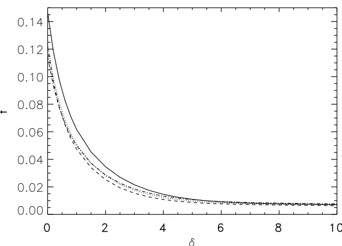
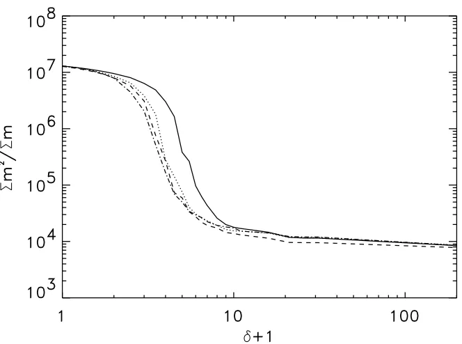
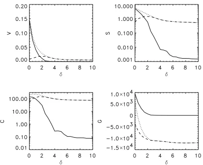
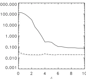
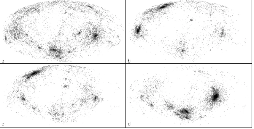
Dreidimensionale Darstellungen der Materieverteilung erlauben es, diese aus einem an-deren Blickwinkel heraus zu untersuchen. Dazu wird die Materie auf ein Gitter verteilt, gegl¨attet, und diejenige Materie, die sich in Zellen befindet, deren ¨Uberdichte4 _{gr¨oßer als ein} Schwellwert ist, wird betrachtet. Einige dieser Zellen sind Teil eines gr¨oßeren Objekts. Ab-bildung A.13 zeigt das gr¨oßte Objekt in der

CDM GIF–Simulation bei einer ¨Uberdichte von 3. Dieses Objekt beinhaltet etwa 30% der Gesamtmasse, f¨ullt etwa 1% des Gesamtvolumens aus und erstreckt sich periodisch ¨uber das gesamte Volumen – ein Effekt, der als Perkolation bekannt ist. Wird der Schwellwert der ¨Uberdichte erh¨oht, schrumpft das Objekt und zerbricht schließlich in viele kleine Objekte. Dieses Verhalten ist typisch f¨ur die CDM–Universen. Eine quantitative Untersuchung des gr¨oßten Objekts ergibt, daß es im wesentlichen aus Filamenten zusammengesetzt ist – wie ja in Abbildung A.13 auch deutlich zu sehen ist.

F¨ur sehr hohe Werte der ¨Uberdichte, etwa 180, bilden die Zellen nur noch sp¨arische oder elliptische Objekte. Die massivsten dieser Objekte entsprechen den bereits erw¨ahnten Gala-xienhaufen. Es zeigt sich, daß sich diese Galaxienhaufen an bevorzugten Stellen innerhalb der Verteilung der Materie bilden: An den Stellen, wo mehrere Filamente oder Sheets aufeinander treffen. Die Materie, die den Galaxienhaufen bildet, str¨omt im zeitlichen Verlauf der Simula-tion entlang der Filamente oder Sheets in Richtung des Haufens. Damit stellen Galaxienhaufen in einem gewissen Sinne bevorzugte Objekte innerhalb der großr¨aumigen Struktur dar. Dies gilt umso mehr, als sie sich, auf der kosmologischen Zeitskala betrachtet, erst sehr sp¨at (etwa bei Rotverschiebungen um 0.3 oder 0.1, je nach dem Wert von) bilden. So kann man z.B.

er-warten, daß man zwischen zwei benachbarten Haufen im Universum ein Filament aus Dunkler Materie finden kann – f¨ur den Fall, daß sich das Universum wirklich durch ein CDM–Modell beschreiben l¨aßt.

1.3.

Pekuliargeschwindigkeiten von Galaxienhaufen

Galaxienhaufen sind nicht nur in Hinsicht auf ihre besondere Lage innerhalb der großr¨aumigen Struktur von Interesse. Zun¨achst einmal sind sie vor allem die massereichsten Objekte, die sich im Universum bislang gebildet haben. Aufgrund ihrer großen Masse mußte Materie aus einer sehr großen Region im fr¨uhen Universum kollabieren. Das bedeutet nun, daß das Dichtefeld im Universum zu dieser Zeit, wenn es auf einer Skala von etwa 10 Mpc/

h

gegl¨attet wird, in den Bereichen, wo Galaxienhaufen entstehen, deutliche ¨Uberdichten haben mußte. Eines der Hauptparadigmen von CDM–Szenarien besagt, daß alle Objekte aus solchen ¨uberdichten Be-reichen, im folgenden wie im Englischen Peaks genannt, entstanden sind und daß die Masse

3_{Die Simulationen enthalten nur Dunkle Materie und keine Galaxien. ¨Ublicherweise werden die gr¨oßten}

Ob-jekte, die in ihnen gefunden werden, mit den gr¨oßten Objekten im Universum, Galaxienhaufen, identifiziert.

eines Objekts im wesentlichen proportional zur H¨ohe eines solchen Peaks ist, wobei mit der H¨ohe eines Peaks schlichtwegs seine ¨Uberdichte mit Bezug auf die mittlere Dichte gemeint ist. Dar¨uberhinaus sollte auch die Geschwindigkeit5eines Peaks, bestimmt ¨uber das gegl¨attete Geschwindigkeitsfeld, mit der des entsprechenden Galaxienhaufens ¨ubereinstimmen. Die Virgo–Simulationen sind ideal, um diese Punkte zu untersuchen, weil sie einerseits eine re-lativ große Region des Universums enthalten und weil es andererseits in ihnen eine gen ¨ugend große Anzahl von Galaxienhaufen gibt.

Die Geschwindigkeitsdispersion in CDM–Universen l¨aßt sich analytisch berechnen, und auch Angaben ¨uber die Geschwindigkeiten von Peaks sind m¨oglich, weil das Spektrum der Modelle, wie oben erw¨ahnt, Gaussisch ist. Die theoretischen Vorhersagen sind hierbei

v(

R

)

H

0

0:6

,1

(

R

)

;

(1.15)

wobei

j f¨ur eine ganze Zahl

j

definiert wird als

2j(

R

)= 1

2

2

Z

P

(

k

)

W

2

(

kR

)

k

2j+2

d

k ;

(1.16)

f¨ur das Integral ¨uber das gesamte Feld und

p(

R

)=

v(

R

) q

1,

40

=

21

2

,1

;

(1.17)

f¨ur Peaks.

W

(

kR

)ist eine Filterfunktion, in der die Gl¨attungsskala gesetzt wird. In den

Sim-ulationen werden Galaxienhaufen als die gr¨oßten Masseansammlungen zur heutigen Zeit ge-funden. Die in ihnen enthaltenen Teilchen werden dann zu alle fr¨uheren Zeitpunkte markiert. Peaks werden ¨uber das gegl¨attete Dichtefeld in den Anfangsbedingungen der Simulationen identifiziert. Die Gl¨attungsskala wird hierbei derart gesetzt, daß sie der minimalen Masse der untersuchten Menge von Haufen entspricht.

Wie in Abbildung 1.1 zu sehen ist, kann der ¨uberwiegenden Mehrheit der Haufen tats¨achlich ein hoher Peak zugeordnet werden. Allerdings ist die Streuung in der Zuord-nung recht betr¨achtlich. Werden die Geschwindigkeit der Haufen in den Anfangsbedin-gungen, denen ein Peak zugeordnet werden kann, verglichen mit der Geschwindigkeit des entsprechenden Peaks, zeigt sich eine exzellente Entsprechung. Gleichermaßen gut ist die

¨

Ubereinstimmung der Geschwindigkeiten der Peaks mit der analytischen Vorhersage (Gl. 1.17). Die Geschwindigkeitsdispersion der Haufen zur heutigen Zeit, direkt gemessen aus der Simulationen, ist jedoch deutlich gr¨oßer als die der Haufen, wenn ihre Geschwindigkeiten aus den Anfangsbedingungen auf die heutige Zeit hochskaliert werden. Insbesondere zeigen Haufen, die einen benachbarten Haufen in einer maximalen Distanz von 10

h

,1Mpc haben,

gr¨oßere Abweichungen, wie in Abbildung 1.2 zu sehen ist.

Im wesentlichen entsprechen also Galaxienhaufen hohen Peaks mit gleichen Geschwindigkeiten im fr¨uhen Universum, wobei massereicheren Haufen im allge-meinen h¨oheren Peaks entsprechen. Allerdings f¨uhren nichtlineare Effekte dazu, daß die Geschwindigkeitsdispersion zur heutigen Zeit deutlich (um 40%) ¨uber der Vorhersage der linearen Theorie liegt.

5_{Im folgenden wird mit der Geschwindigkeit einer Objekts grunds¨atzlich seine Pekuliargeschwindigkeit}

Abbildung 1.1.: Die Massen der Galaxienhaufen in den vier Simulationen in Abh¨angigkeit der H¨ohe der ihnen entsprechenden Peaks. Es gibt 351, 239, 84, und 83 Peaks ohne zugeh¨origen Haufen in der SCDM,

CDM,CDM, und OCDM–

Simulation. 85% und 75% der Haufen in den Modellen mit=1und

<

1

konnte ein Peak zugeordnet werden.

1.4.

Simulationen des Hubble Volumens

Die ideale kosmologische Simulation w¨urde das gesamte beobachtbare Universum enthalten mit einer sehr hohen Massenaufl¨osung. Dies w¨are insbesondere f¨ur das Studium sehr sel-tener Objekte, wie z.B. Galaxienhaufen, von Interesse. Im Rahmen dieser Arbeit wurden zwei Simulationen, die sog. Hubble–Simulationen, durchgef¨uhrt, die diesem Ideal relativ nahe kom-men. Beide Simulationen enthalten einen signifikanten Bruchteil des gesamten beobachtbaren Universums und sind um mindestens eine Gr¨oßenordnung gr¨oßer als die n¨achste Generation von sehr umfangreichen Galaxienkatalogen. Damit wurde es zum ersten Mal m¨oglich, Eigen-schaften von Galaxienhaufen zu untersuchen, die bislang jenseits der M¨oglichkeiten von Sim-ulationen lagen.

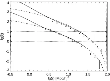
Abbildung 1.3 zeigt die differentielle Anzahldichte von massereichen Galaxienhaufen bei einer Rotverschiebung von

z

= 0

:

78. Die Anzahl der Beobachtungen solcher Haufen ist

deut-Abbildung 1.2.: Vergleich der Geschwindigkeiten der Galaxienhaufen zur heutigen Zeit (

v

z=0) mit der auf die heutige Zeit hochskalierten Geschwindigkeit aus den Anfangs-bedingungen (

v

_{scaled). Galaxienhaufen, die einen benachbarten Haufen in} einer maximalen Distanz von10

h

,1Mpc haben, sind durch die Rauten

ken-ntlich gemacht.

lich zu sehen ist, ist die

CDM–Simulation nicht in der Lage, solch massereiche Objekte zu bilden. Mit anderen Worten bildet sich Struktur in einem Universum mit = 1viel zu sp¨at.

DasCDM–Modell bildet mehr massereiche Galaxienhaufen bei

z

=0

:

78, allerdings befindet

sich ein beobachteter Haufen weit außerhalb der Verteilung. Derzeit sind die Bestimmungen der Massen solcher Haufen noch immer strittig, so daß es zum heutigen Zeitpunkt nicht ange-bracht erscheint, ein endg¨ultiges Urteil ¨uber dasCDM–Modell zu f¨allen.

Abbildung 1.4 vergleicht die Massenfunktion der

CDM–Simulation mit der theoreti-schen Vorhersage des Press–Schechter–Modells. Die Simulation l¨aßt sich in der Tat sehr gut mit diesem Modell beschreiben. Die Abweichungen, die in der Abbildung zu sehen sind, entsprechen denen, die bislang in kleineren Simulationen gefunden worden sind. Sie sind in-sofern kein Grund zur Sorge, als es a priori ¨uberhaupt keinen Grund gibt, warum das Press– Schechter–Modell die Massenfunktion ¨uberhaupt so gut beschreiben soll.

14.2

14.4

14.6

14.8

15.0

log(m)

10

-10

10

-9

10

-8

10

-7

10

-6

N [h

3

Mpc

-3

]

Abbildung 1.3.: Die differentielle Anzahldichte von Galaxienhaufen bei einer Rotver-schienung von

z

=0

:

78in der

CDM (durchgezogene Linie) und derCDM

(gestrichelte Linie) Simulation. Die Massen sind innerhalb eines Radius von 0.5 Mpc/

h

bestimmt worden. Die drei Meßpunkte geben drei beobachtete Objekte im Universum wieder.

Simulationen erstellt wurden, sind ideal, um dies zu untersuchen. Hierzu wird die Zwei– Punkt–Korrelationsfunktion,

(

r

), benutzt. F¨ur jeden Haufen gibt sie an, wieviel

wahrschein-licher es ist, bei einer Entfernung

r

einen zweiten zu finden, als wenn die Haufen poisson-verteilt im Raume w¨aren. Die Korrelationsl¨ange,

r

_{0, ist definiert ¨uber}

(

r

0) = 1. Da

Gala-xienhaufen im Universum so selten sind, ist es ¨außerst schwer, einen Katalog zu erstellen, der vollst¨andig ist. ¨Ublicherweise sind Kataloge nur vollst¨andig ab z.B. einer bestimmten R¨ontgenleuchtkraft der Haufen. Deswegen wird die Korrelationsfunktion gemessen als Funk-tion der Dichte,

n

_{c, des Katalogs, der ¨uber}

d

_c =

n

,1=3

c ein mittlerer Abstand der Haufen entspricht. Die Abh¨angigkeit der Korrelationsl¨ange von der Haufendichte ist derzeit noch um-stritten, und erst mit den Hubble–Simulationen stehen ausreichend große simulierte Kataloge zur Verf¨ugung, um dies zu untersuchen.

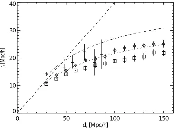
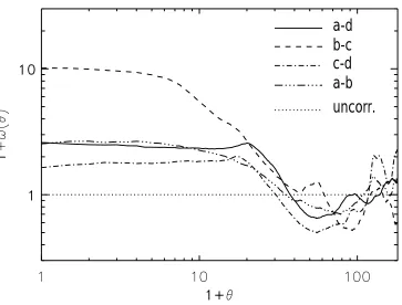
Abbildung 1.5 zeigt die Korrelationsl¨angen der Galaxienhaufen in der

CDM (K¨astchen) und derCDM (Rauten) Simulation in Abh¨angigkeit der Dichten von Teilmengen der

Kata-loge. Ebenfalls gegeben sind f¨ur die beiden Modelle (gestrichelte und strichpunktierte Linie) die Vorhersagen des Modells von Mo & White (1996). Dieses dr¨uckt die Korrelationsfunktion der Haufen aus ¨uber

(

r

)=

b

2

13.0 13.5 14.0 14.5 15.0 15.5 16.0 lg(M)

-10 -8 -6 -4 -2

lg(n(>M))

z=0 z=0.44 z=0.78

Abbildung 1.4.: Die kumulative Massenfunktion in der

CDM–Simulation (Kreuze) f¨ur drei verschiedene Rotverschiebungen. Die Kurven geben die theoretische Vorher-sage wieder.

mit

b

(

R

)=1+

c

2(

R

) ,

1

c

:

(1.19)

Hierbei ist

DM(

r

)die Korrelationsfunktion der Dunklen Materie, und

b

(

R

)ist ein

sogenan-nter Biasfaktor. Dieser bestimmt sich aus der Konstanten

_c = 1

:

69 und aus dem Moment

2(

R

)(entsprechend

j

=0in Gleichung 1.16).

R

ist wie oben der Radius, der der minimalen

Haufenmasse entspricht. Ebenfalls abgebildet sind in Abbildung 1.5 ein linearer Zusammen-hang zwischen der Korrelationsl¨ange und der Haufendichte (gestrichelte Linie) und das Ergeb-nis der Analyse der Galaxienhaufen im APM–Katalog (Kreuze; Croft et al. 1997). Wie deut-lich zu sehen ist, ist das lineare Modell nicht vereinbar mit den Vorhersagen der Modelle und der Messung. Die Theorie von Mo & White sagt zu große Korrelationsl¨angen voraus, stimmt qualitativ aber mit den Ergebnissen aus der Simulation ¨uberein. Von den beiden Simulationen stimmt wieder nur dieCDM–Simulation mit der Messung ¨uberein.

0 50 100 150 dc [Mpc/h]

0 10 20 30 40

r0

[Mpc/h]

Abbildung 1.5.: Die Korrelationsl¨ange der Galaxienhaufen in Abh¨angigkeit des mittleren Ab-stands der Haufen (mithin als Funktion der Dichte der Haufen). Die Boxen und Rauten sind die Ergebnisse aus der

CDM und der CDM–Simulation.

Bibliography

[1] Bond J.R., Efstathiou G., ApJ 285, L45 (1984)

[2] Croft R.A.C., Dalton G.B., Efstathiou G., Sutherland W.J., Maddox S.J., astro-ph/9701040

[3] de Lapparent V., Geller M.J., Huchra J.P., ApJ, 302, L1 (1986)

[4] Davis M., Efstathiou G., Frenk C.S., White S.D.M., ApJ, 292, 371 (1985)

[5] Haynes M.P., Giovanelli R., ApJ, 306, L55 (1986)

[6] Mo H.J., White S.D.M., MNRAS, 282, 347 (1996)

Chapter

2

Introduction

C’est une maladie naturelle `a l’homme de croire qu’il poss`ede la v´erit´e directement; et de l`a vient qu’il est toujours dispos´e `a nier ce qui lui est in-compr´ehensible.

Blaise Pascal

Over the last twenty years, cosmology has evolved from a rather speculative side branch of astrophysics and philosophy into a high precision science of its own. This is due to the fact that, recently, an amount of knowledge has been gained which is so large compared with what was known earlier that is probably not too much of an exaggeration to compare this process with the development of quantum mechanics and its subsequent revolution of atomic physics in the early decades of the 20th century.

Observationally, new technology in the form of satellites and telescopes and also new tech-niques in order to study objects have arisen which have revolutionized our understanding of the Universe. For instance, the Cosmic Microwave Background Explorer (COBE) satellite has measured the afterglow of the Big Bang with a precision undreamt of before. It shows that the Microwave Background (CMB) has a nearly perfect black body spectrum and that there must have been fluctuations of the order of10

,5 in temperature (and thus in density) in the very early

Universe. The Hubble Space Telescope (HST) has widened the view of not only cosmology, but of the whole field of astrophysics. Combined with new ground based telescopes like for the Keck, galaxies at a redshift of five, that is, at a time when the Universe had only a sixth of its current age and size, can now be found. The existence of Dark Matter in galaxy clusters can be observed by means of gravitational lensing. This very short list gives only a few highlights of the new data which theories about the birth of the Universe and the subsequent formation and evolution of galaxies and Large–Scale Structure have to explain.

for the Universe, some of them are not very wrong. So theoreticians have to start fine tuning their models – something unknown to the field before. Computer simulations have played a major rˆole in this process. This is not only due to the truly gigantic increase in computational power over the last decades. For instance, the Hot Dark Matter model, which assumes that the dominant (and unseen) mass component in the Universe consists of massive neutrinos1_{, was} rejected on the basis of a simulation with only 1000 particles (White et al. 1983). The seminal simulation work of Marc Davis, George Efstathiou, Carlos Frenk, and Simon White in 1985 (DEFW hereafter) with323 Cold Dark Matter particles contains results which are still valid

today. However, larger simulations are still needed to increase the predictive power of the the-ories. Larger regions of the Universe have to be simulated with a higher mass resolution to test cosmological models further.

This work is about some of these high precision simulations. In the remaining sections of this Chapter, the basic theoretical foundations will be laid. Section 2.1 briefly describes the set of fundamental cosmological equations and variables used throughout the whole work. Section 2.2 gives an overview of the growth of perturbations. Finally, section 2.3 contains an introduc-tion into the family of Cold Dark Matter models used in the simulaintroduc-tions themselves.

Chapters 3 and 8 contains the technical part of this work. They describe some details of the computers, the codes used, and the simulations themselves.

In Chapter 4, the large–scale distribution of the mass in the simulations is studied. The density field, smoothed on suitable large scales, is investigated as a function of the mass above an overdensity threshold.

Chapter 5 contains a study of the most massive objects in the simulations. These are iden-tified similarly to how observers find galaxy clusters. The main point of the Chapter is to de-termine if peculiar velocities of galaxy clusters can be predicted accurately. To this end, the correspondance between peaks in the smoothed initial density field and clusters is studied.

In Chapter 6, the Hubble Volume Simulations are introduced. These represent the biggest effort in computational cosmology to date and will be the basis for predictions for the next gen-eration of very large galaxy surveys. Catalogs of galaxy clusters which each contain hundreds of thousands of clusters are extracted and used to study the existence of massive objects at high redshifts and the mass function itself (section 6.3), and cluster correlation functions (section 6.4).

Chapter 7 links the themes of the earlier Chapters. It shows how the formation process of galaxy clusters is linked to the mass distribution around the clusters, that is, to Large–Scale Structure itself. Finally, Chapter 9 contains a summary of this thesis.

2.1.

Basic Cosmology

H¨uten wir uns, zu sagen, daß es Gesetze in der Natur gebe. Es gibt nur Notwendigkeiten: da ist keiner, der befiehlt, keiner, der gehorcht, keiner, der ¨ubertritt. Wenn ihr wißt, daß es keine Zwecke gibt, so wißt ihr auch, daß es keinen Zu-fall gibt: denn nur in einer Welt von Zwecken hat das Wort ”Zufall” einen Sinn.

Friedrich Nietzsche,

Die Fr¨ohliche Wissenschaft, III, 109

The Big Bang as the origin of the Universe is now a well–established theory. According to this theory, at some time in the distant past, space and time originated from the expansion of a tiny region. In this section, it is assumed that the result of this process is a Universe which is smooth and homogeneous on very large scales. This implies that the Universe essentially looks the same at all spatial locations, there is no preferred region in the Universe – something called the ”Copernican Principle”. The theory which describes the dynamics of the gravita-tional field is Einstein’s theory of General Relativity. The spacetime metric for such a Universe is the Friedmann–Robertson–Walker (FWR) metric2

d

s

2

=(

c

d

t

)

2

,

a

2

(

t

) "

d

r

2

1,

kr

2

+

r

2 (d

#

2 +sin 2

_#

d

2 ) #

:

(2.1)

Here,

a

(

t

), the so–called expansion factor, and

k

are determined using Einstein’s equation.

k

may take three different values, namely

k

=1, 0, and,1for positive, zero, and negative

curva-tures of spatial hypersurfaces, respectively. The time dependance of

a

implies that any proper distance scale

l

(

t

)is proportional to it

l

(

t

)/

a

(

t

)

:

(2.2)

This implies that electromagnetic radiation will change its frequency as it travels across the Universe. As

a >

_ 0, an observer will receive spectra from distant objects which are reddened.

If the observed and emitted frequencies are named

!

_{0 and}

!

_{e, respectively, then the redshift}

z

is be defined via

!

e

!

0 = 1

a

(

t

e)

1+

z ;

(2.3)

where

t

_{e denotes the time of emission, and}

a

(

t

)has been normalized such that it is unity today,

i.e.

a

(

t

0)=1.

As indicated above,

a

(

t

)and

k

can be computed from Einstein’s equations

G

=8

GT

;

(2.4)

2_{The following discussion can be found in most textbooks on cosmology, e.g. Padmanabhan 1993. Note, that}

if the stress–tensor

T

for the source of the gravitational field is given. Matter is usually treated as a perfect fluid which is specified by a pressure

p

and a density

. Using the FRW metric (2.1) and the assumption of homogeneity and isotropy (which makes all non–diagonal elements of

T

vanish) then yields two independent equations, viz.3

_

a

2

+

k

a

2 =

8

G

3

;

(2.5)

2 

a

a

+ _

a

2+

k

a

2 = ,8

Gp:

(2.6)

The overdot denotes differentiation with respect to time.

a

(

t

)

;

(

t

)

;

and

p

(

t

)are fully specified

once the equation of state

p

=

p

(

)is given. Using the following three abbreviations

H

0 _

a

a

t=t0 (2.7)

c

3

H

20

8

G

(2.8)

0

0

c (2.9)

yields that at present epoch

k

=

H

2

0(0,1)

:

(2.10)

H

0 is called the Hubble constant at present time,

c is the critical density, and0 is the density

parameter. From equation (2.10) it is obvious that these parameters determine the curvature of the Universe. 0 =1gives a flat Universe.

Combining equations (2.5) and (2.6) gives



a

a

=,

4

G

3

(

+3

p

)

;

(2.11)

which implies that 

a <

0 for ordinary kinds of matter, which have(

+3

p

)

>

0.

a

thus is

smaller in the past and will become zero at some finite time in the past (Big Bang). Integration yields the age of the Universe:

t

0 = 2

3 1

H

0

f

(0)

;

(2.12)

where

f

(0)=1for0 =1and

f

(0)

>

1for0

<

1. Furthermore, one can show that for

0 =1

a

/

t

1=2 _(2.13)

a

/

t

2=3 _(2.14)

for the radiation–dominated and matter–dominated phases of the Universe, respectively4. Gen-erally, the equations are easy to solve analytically for0 =1and need to be done numerically

otherwise.

3

c=1has been set here.

4_{The Universe is called radiation (matter) dominated when the energy density of radiation (matter) dominates.}

A further concept has to be introduced here. The source term for Einstein’s equations (2.4) can be any conserved stress–tensor. In particular, one can take

T

ik =

ik

;

(2.15)

whereis the so–called Cosmological Constant postulated, and later abandoned, by Einstein.

He originally wanted to have a stable, i.e. non–expanding Universe, but quite obviously this doesn’t work because small fluctuations around the ”stable” state would result in an immediate collapse (or in an immediate expansion). corresponds to an equation of state

p

=,

=,.

By noting its contribution to the density in the Universe

0 =

8

G

3

H

20

(2.16)

one can take this as the vacuum energy density. Crudely speaking, doesn’t change the

ex-pansion of the Universe at early times. At later times it starts to accelerate the exex-pansion. The age of the Universe is increased relative to a Universe with0 =1. A non–vanishingis

em-barrassing because there is no good physical explanation for its existence and no convincing explanation why it should have the value favoured by some cosmologists (for further discus-sion see section 2.3.5).

2.2.

The Growth of Perturbations

In the preceding section, it was assumed that at early times the Universe was smooth and ho-mogeneous on large scales. From the fact that e.g. galaxies exist today it is obvious that it can not be smooth and homogeneous on small scales. Deviations from homogeneity must have existed in the early Universe from which all objects seen today must have formed. Objects in the gravitational instability scenario formed from the collapse of overdense regions. COBE does indeed find such fluctuations on the Microwave Sky, they are small (

T=T

10

,5), but

nevertheless they must have been big enough to cause the collapse of structure.

Consider a pressureless fluid with density

and velocityvunder the influence of a

gravi-tational field with potential

5_{. The equations which describe this fluid are}

@

@t

+r(

v) = 0

;

(continuity) (2.17)

@

v

@t

+(vr)v = ,r

;

(Euler) (2.18)

r

2

= 4

G:

(Poisson) (2.19)

These equations can be cast into a cosmological context by using appropriate variables. These are a comoving positionx=r

=a

, which is fixed for an observer moving with the Hubble

expansion, and the corresponding peculiar velocity u =

a

dx

=

d

t

, representing departures of

the matter motion from pure Hubble expansion.

Assume the density is spatially variable

(x

;t

)=

(

t

)(1+

(x

;t

))

:

(2.20)

Then equations (2.17) to (2.19) can be transformed from the coordinate systemrtoxwhich

gives

@

@t

+ru+r(u

) = 0

;

(2.21)

@

u

@t

+(ur)u+2 _

a

a

u = ,r

=a

2

_;

_(2.22)

r

2

=a

2

= 4

G

:

(2.23)

In these equations,rand the overdot now denote differentiation w.r.t.xand time, respectively.

Perturbations in the early Universe must have been small. One can thus combine equations (2.21) to (2.23) and neglect all non–linear terms to get



+2 _

a

a

_

,4

G

=0

:

(2.24)

For0 =1, equation (2.24) can be solved easily. In this case,

a

/

t

2_{=3, which gives}



+ 4 3

t

_

, 2

3

t

2

=0

:

(2.25)

Obvious solutions for equation (2.25) are

/

D

(

t

)/

t

2=3

/

a

(growing mode) (2.26)

/

a

,3=2

(decaying mode) (2.27)

D

(

t

)is the so–called growth factor of fluctuations. For0

<

1, the solution is more

compli-cated. It can be shown that at early times when1the decaying and growing mode behave

as in the case where0 = 1. At late times, when

<

1, the growing mode starts to saturate

and structure ceases to grow.

The growth of peculiar velocities is studied in Chapter 5. After some algebra, the equations above show that the peculiar velocity of every mass element grows as

v/

a

_

D :

(2.28)

According to Heath (1977), the growth factor for a general cosmology is given by

D

=

H

,2

0

X

1=2

a

,1

Z a

0

X

,3=2

d ~

a;

(2.29)

where

X

1+0(

a

,1

,1)+0(

a

2

,1). The subscript ”0” now explicitly refers to the

values of the density parameter and the cosmological constant at the present time. A number of accurate approximate forms are known for the relations between

D

and

a

.

D

_ can be re–

written as follows

_

D

d

D

d

t

= d

D

d

a

d

a

d

t ;

whered

a=

d

t

can be substituted from the Friedmann equation. Lahav et al. (1991) give an

ap-proximation ford

D=

d

a

:

f

(

a

)

d

D

d

a

a

D

0

a

,3 0

a

,3

+(1,0 ,0)

a

,2

+0

!0:6

:

(2.31)

For

a

=1this gives the standard factor

f

0:60 which appears when predicting the peculiar

velocities produced by a given overdensity field. Carroll et al. (1992) used this result to derive an approximation for

D

(

a

)itself,

D

ag

(

a

)

;

(2.32)

where

g

(

a

)= 5

2

(

a

)

4=7(

a

),(

a

)+

1+ (a) 2 1+ (a) 70 (2.33) with

(

a

)

0

a

+0(1,

a

)+0(

a

3,

a

)

;

(2.34)

(

a

)

0

a

3

a

+0(1,

a

)+0(

a

3,

a

)

:

(2.35)

Combining these equations, yields an explicit approximation for the growth of peculiar veloc-ities:

v/

f

(

a

)

g

(

a

)

a

2q

0

a

,3

+(1,0,0)

a

,2

+0

:

(2.36)

For the simple case where 0 = 1and 0 = 0, these formulae reduce to the exact results

D

=

a

/

t

2=3 andv/ p

a

.

2.3.

The Cold Dark Matter Model

2.3.1.

Introduction

According to the standard theory in cosmology described above, the Universe was born in the Big Bang, i.e. it was hot, dense, and homogeneous in the beginning, from whence it expanded adiabatically according to the laws of General Relativity. However, this picture is incomplete, for it does not explain why on small scales, say a few Megaparsecs (Mpc), matter is clumpy and not distributed homogeneously. In addition, evidence is growing that the amount of matter which emits electromagnetic radiation and thus can be seen in the Universe, is far less than the amount of matter which must be there. The visible matter can only account for a small fraction of the total mass: Dark Matter shows up via its gravitational influence on various scales.

2.3.2.

Dark Matter

Why Dark Matter?

Evidence for the existence of matter which does not emit electromagnetic radiation at any wavelength and which only shows up via the influence of its gravity (Dark Matter) comes from different scales:

Scales of galaxies (a few ten kpc): The rotation curves of spiral galaxies, i.e. the rota-tion speed as a funcrota-tion of the distance from the galactic center, are flat at large distances, contrary to the prediction of Kepler‘s law which would give a decreasing rotation speed for the visible matter. However, if a spherically distributed Dark Matter component is added, which is larger than the disk itself, a so–called halo, the observed rotation curve for radii larger than a few kpc is dominated by the halo and can be flat.

Scales of galaxy clusters (a few Mpc): The relative amount of Dark Matter is greater for galaxy clusters6. The total mass of a galaxy cluster can be found either by using the galaxies as test particles in the system‘s potential and deducing the mass from their ve-locities, by converting the X–ray emission of the hot intracluster gas into a mass estimate, or by means of gravitational lensing where the deflected light of background galaxies is used to infer the mass of the cluster. The latter method is free of assumptions (whereas the former two assume virial equilibrium which is not necessarily true). However, it mea-sures the projected mass which could be contaminated by objects lying behind or in front of clusters. The methods agree relatively well for a large sample of clusters and if one compares the total mass with the mass of the baryons (which is believed to mainly consist of the galaxies themselves plus the hot intracluster gas) one finds that the baryon fraction is around 10 to 20% (White et al. 1993a).

Very large scales (tens of Mpc): The assumption that galaxies may be treated as test par-ticles allows a reconstruction of the cosmic velocity field from which the potential of the underlying mass distribution can be deduced. Using Poisson’s equation then gives the density field which can be compared to the observed density field of the galaxies. From this procedure, evidence is mounting that not only is the visible mass just a small fraction of the total mass, but that the total mass may be close to the critical amount required to make the Universe flat, i.e.0 =1(e.g. Dekel 1994).

These observations directly lead to the question:

What is the Dark Matter?

The simplest approach to solve the Dark Matter problem is to assume that the Dark Matter is the same type of matter as that which has already been seen, i.e. baryons. Objects which consist of baryons but do emit little if any light are well known: they include for instance brown dwarfs.

6_{The uusal way of expressing this is to give the ratio of the mass of and the light emitted by an object, the so–}

called mass–to–light–ratioM=L. Typical values areM=L30M

=L

and

M=L300M

=L

for

galax-ies and galaxy clusters, respectively, whereM

and

L

However, a strong upper and lower limit on the amount of baryons in the Universe comes from Primordial Nucleosynthesis. According to this theory,

0

:

009

h

,2

b 0

:

02

h

,2

(2.37)

which is inferred from measured abundances of light elements (e.g. Copi et al. 1995). Hence, unless a severe error in these computations and measurements shows up, the Dark Matter can not consist of ordinary baryons unless0 is very small.

Almost all remaining Dark Matter candidates have one thing in common: They are elemen-tary particles. Usually they are classified according to their speed when galaxy–sized fluctu-ations entered the horizon. Particles which were relativistic (non–relativistic) at that time are named Hot (Cold) Dark Matter.

Hot Dark Matter is probably the most straightforward solution for the Dark Matter problem, simply because neutrinos with a non–vanishing mass would have been relativistic when they decoupled from the rest of the matter in the Universe. In addition, neutrinos are known to exist. However, their masses are unknown. The mass of a neutrino must not be larger than about 30 eV – otherwise neutrinos would overclose the Universe. Although the neutrino masses are not known, it is already clear that neutrinos can not be the dominating Dark Matter component7_. If 1then the free streaming of the neutrinos would have destroyed any adiabatic density

fluctuation smaller than the size of superclusters (1015

M

) in the early Universe (Bond et al.

1980). As a consequence, structure would have formed in a so–called top–down scenario, with superclusters forming first and galaxies forming only at the present epoch. As high redshift galaxies are have been observed, this model cannot explain the formation of structure in the Universe. In addition, this model is incompatible with the fluctuations in the CMB.

As a consequence of the above, Cold Dark Matter (CDM) remains the best Dark Matter can-didate. There are no known (i.e. detected) elementary particles which could be CDM. However, the list of postulated CDM particles is long. Most of these particles are either Weakly Interact-ing Massive Particles (WIMPs). There are two reasons why one should not worry about the fact that neither of these types of particles has been detected yet. First, the neutrino itself was pos-tulated by Wolfgang Pauli long before it was detected – which shows that postulating particles on a solid physical ground is much more than science fiction. And second, particle physicists themselves are thinking of elementary particles beyond the standard model of particle physics; the masses of some of these particles fit nicely into the cosmological mass estimates.

Whatever CDM actually consists of, the important point is that, from the viewpoint of cos-mology, there is a need for these particles, which are well motivated within almost all exten-sions of the standard model of particle physics. Thus, one of the main hypotheses of this work is that Dark Matter consists entirely of CDM8.

7_{This holds if the density fluctuations were generated during inflation. Hot Dark Matter could work in the context}

of string cosmologies but this is beyond the scope of this work.

8_{It may be argued that there may be a small contribution of Hot Dark Matter if}

0

= 1. For details on the

2.3.3.

Inflation as the Origin of Fluctuations

Introduction

Currently, there are two competing scenarios for the generation of density fluctuations needed to trigger gravitational collapse. These are Inflation and Topological Defects. Due to its com-plexity, the latter is neither as well understood nor has it been investigated in as much detail as the former. As Inflation is taken as the scenario which generates density fluctuations, Cosmic Defects are not discussed here.

Inflation

The first and very simple question is: Why would there be density fluctuations at all after the Big Bang? Suppose one assumes that there must have been some fluctuations because this is the only way to explain why the Universe is not completely homogeneous on small scales but contains galaxies, galaxy clusters, and voids. Then the next question that arises is: If causality holds, how can the temperature variation of the CMB be only about

T=T

10

,5 from

re-gions on the sky which were causally disconnected at recombination? And why is the Universe so close to being flat, i.e. why istot 1(neglecting for the moment the debate about its actual

value)? In addition, after the phase transition in the very early Universe (symmetry breaking) a huge number of topological defects such as monopoles should have been created; why is the density in these monopoles so low today? In addition, one may wonder what the details of the density fluctuations are? How can they be described in a statistical sense, i.e. what does the density fluctuation spectrum look like? Inflation provides answers to all these questions in a rather simple fashion which allows one to connect the measurements of the CMB with detailed models.

In spontaneously broken gauge theories which are used to describe the state of the very early Universe, the vacuum energy plays a very important role. It can be described as an cos-mological constant. The idea, first proposed by Guth (1981), is to let this vacuum energy inflate a single causally connected region in a de Sitter–like cosmology to a gigantic scale.

Consider a very simple universe which could look like this: It is empty (i.e.

= 0), has

a vanishing curvature (

k

= 0), and a positive cosmological constant (

>

0) – the de Sitter

cosmology. The solution of Friedmann‘s equation is then simply

a

=

a

0exp [

Ht

]

;

(2.38)

where the Hubble parameter is constant

H

= q

=

3. Thus, this universe would expand

expo-nentially due to the effective pressure of space time itself which is described by.

It can be shown that this period of inflation not only solves the flatness problem, in addition

tot = 1is nearly inevitable – some extra work is required to allow an open cosmological

model with tot

<

1(c.f. Turok & Hawking 1998). The monopole problem is also solved

of different regions of the same size complete the phase transition to the Friedmann phase at different times. This time spread

t

=

_

can be obtained from the equation of motion of

(which is the free Klein–Gordon equation in an expanding universe) and it is directly con-nected to the density fluctuations

_H =

=

/

H

t

. Now the assumptions which have to

be made for the inflaton field (essentially inflation has to last long enough in order to achieve its goals – the so–called slow roll approximation – so that the potential must not vary much) yield

H =constant. Thus, inflation predicts a constant curvature spectrum

H =constant of

adiabatic fluctuations (known as Zel‘dovich spectrum). In addition, the quantum fluctuations in

have random phases and therefore are Gaussian.

It should be noted again that newer variants of inflation manage to result intot

<

1, too.

This may be important because it is not yet clear that tot = 1. So inflation not only solves

some nasty problems but predicts the spectrum of density fluctuations to be

P

(

k

) /

k

. One

of the disadvantages it has is that it cannot uniquely predict the amplitude of the fluctuations. There are many variants of inflation each having different choices of

. They vary in different aspects and some of them produce results which are unlikely to be testable. However, they all have the above features in common and all yield different amplitudes. This leads to the question of how this amplitude can be determined from observations.

2.3.4.

The Fluctuation Spectrum and the Amplitude of Mass

Fluc-tuations

In addition to the generation of the primordial spectrum of density fluctuations a second phys-ical process must be taken into account. Small scale density pertubations (with

<

_eq) enter the horizon prior to the epoch of equivalence between matter and relativistic particles (

eq 13

=

0

h

2 Mpc is the comoving horizon scale at that epoch). They are damped and the

spectrum develops a bend at the scale

_{eq. The processes which change the shape of the} primor-dial fluctuation spectrum are usually combined in the so–called transfer function

T

(

k

)which

relates the primordial spectrum to the actual spectrum through:

P

(

k

)=

T

2

(

k

)

P

p(

k

)

;

(2.39)

where

P

_p(

k

)now denotes the primordial spectrum and

P

(

k

)the actual one.

The parametric form for

T

(

k

) used in this work was introduced by Bond & Efstathiou

(1984). In their notation, the power spectrum is given by

P

(

k

)=

Ak

(1+[

ak=

,+(

bk=

,)3=2+(

ck=

,)2])2=

;

(2.40)

where

a

= 6

:

4

h

,1 Mpc,

b

= 3

:

0

h

,1 Mpc,

c

= 1

:

7

h

,1 Mpc, and

= 1

:

13.

A

is the yet

unknown normalization and,gives the typical scale of the spectrum. This is,=0

h

for all

pure CDM models (for a CDM model which deviates from this see section 2.3.5).

fluctuations in the mass distribution on scales of 8

h

,1 Mpc,

8, defined by

₈2

1

(2

)3

Z

P

(

k;

,)

3

kR

8

j

1(

kR

8)

2

d

3

_{k ;}

_(2.41)

where

R

₈ =8

h

,1 Mpc, and

j

1 is a spherical Bessel function.

COBE has an angular resolution of about 7

which corresponds to scales much larger than any scale of interest in current cosmological investigations and simulations. Hence, a model which links these scales to much smaller ones is needed. This cannot be done unambiguously. For example, the amount of gravitational waves is still uncertain in inflationary scenarios. This could change

A

dramatically. Obtaining values for

A

from the mass distribution on cluster scales does not suffer from this problem. The basic idea behind this is rather simple: The mass function, that is the number of objects of some mass as a function of mass, is falling very steeply at its high mass end, i.e. high mass objects like rich clusters of galaxies are very rare (compare Chapter 6). As the mass function itself depends on the amplitude of fluctuations, the overall amplitude

A

of the power spectrum can be fixed by matching the observed abundance of rich clusters in computer simulations.

Values for

_{8 can be obtained by using either the mass (White et al. 1993b) or the X–ray} temperature functions (Eke et al. 1996, Viana & Liddle 1996) of rich clusters. The different studies carried out this way more or less agree that

8 0

:

6

,0:6

0

:

(2.42)

2.3.5.

Cold Dark Matter Models

Die Welt ist unabh¨angig von meinem Willen.

Ludwig Wittgenstein Tractatus logico–philosophicus 6.373

In the following, the four models used in the VIRGO simulations will be introduced. In addition, some of their features will be discussed. A concluding section summarizes the present

status quo of measurements of the density parameter0. Despite several indications at this

time no decisive point can be made whether or not the density parameter is unity or smaller than unity.

SCDM

In principle, the simplest cosmological model, named Standard CDM (SCDM), is a no para-meter model where all quantities are fixed either from the predictions of inflation or from mea-surements. These are

n

= 1,0 = 1, and

h

=0

:

5

9_.

h

_{cannot be chosen to be larger because} otherwise the age of the Universe would be smaller than the age of the oldest stars. This is still very uncertain, though. For a recent review of determinations of the Hubble Constant c.f. Branch (1998). As introduced above, SCDM has,=0

h

=0

:

5.

9_{The Hubble constant is usually expressed as}

H 0

Nowadays, it has become en vogue to state that the SCDM model does not work and that it has to be substituted by some variant. But SCDM in most cases is wrong only by a factor of two or so – which is rather small compared with the usual uncertainties in astrophysics/cosmology. So what actually is wrong with SCDM? As already stated in section 2.3.4, the normaliza-tions obtained by COBE and via clusters disagree strongly. The amount of small scale power relative to large scale power is too large. Thus, if normalized to COBE, SCDM predicts too high an abundance of galaxy clusters. If normalized to give the correct abundance of clusters, the correlation function is too steep (Davis et al. 1985, Jenkins et al. 1998) and COBE fluc-tuations are underpredicted. Problems like this show up in many other topics (galaxy–galaxy and cluster–cluster correlation functions (Bahcall & Cen 1992, Efstathiou et al. 1990), genus statistics (Springel et al. 1997) to name just a few. For a detailed discussion of this topic c.f. Ostriker 1993). Probably the simplest way to understand why SCDM has these problems is its typical scale, specified by,=0

:

5. On the basis of galaxy clustering, Peacock & Dodds (1994)

found,0

:

25. Thus, the power spectrum of SCDM has a peak which is at too large a wave

number. From this it is clear why the above normalization problems show up.

CDM

As indicated above,,0

:

25is needed to match the clustering statistics of galaxies and galaxy

clusters. For a model with0 =1this cannot be easily achieved without invoking additional

physics because the obvious solution, to lower the Hubble constant to

h

=0

:

25, is in conflict

with observational limits (Bartlett et al. 1995). One possibility is to assume that massive neutri-nos which existed in the early Universe have now decayed into other neutrineutri-nos. The

neutrino is a candidate for such a particle, hence the name of the model. A decaying neutrino species leads to an enhancement of the content of relativistic particles in the Universe. This changes the power spectrum of density fluctuations. In any model without such a decay process, the early Universe is radiation dominated, but matter starts to dominate later because the densities of radiation and matter scale differently with

a

. In the

CDM model this process is changed as follows. In the early stages of the Universe the energy density of the massive neutrinos is the same as that of a massless species. As the Universe expands, the massive neutrinos become nonrelativistic, and their energy density starts to increase relative to their massless counter-parts. This leads to an epoch in which the density of the Universe is dominated by massive neutrinos. Later, they decay, and their rest energy is converted into energy for relativistic par-ticles – thereafter the Universe starts to evolve like a SCDM Universe, but with a higher energy density in relativistic particles which causes equipartition to occur later hence reducing,.

The shape parameter,of the power spectrum can be expressed as follows (Bardeen et al.

1986):

,'m0

h

r0

h

2

4

:

1810

,5 !

,1=2

:

(2.43)

r0 =

r0

=

crit, where

r0 is the present energy density in relativistic particles, andm0 stands

for the matter that can clump at small scales. For SCDM (wherer0 =4

:

1810 ,5,

m0 0)

, = 0

:

5as introduced above. An increase in the density of relativistic particles – as in the

spectrum, the necessary density in relativistic particles has to be achieved.

It can be shown that,is a function of the mass and the lifetime of the massive neutrinos

as follows

,=0

h=

[0

:

861+3

:

8(

m

2 10

)

2=3

]

1=2 _(2.44)

This fitting formula is given by White et al. (1995).

m

_{10 is the mass of the neutrino in units of} 10 keV and

is its lifetime in years. Obviously, the

CDM model requires additional physics beyond the Standard Model of High Energy Physics. For more details about scenarios with decaying neutrinos and their cosmological implications c.f. Bharadwaj & Sethi (1998).

The parameters of the Virgo

CDM model are 0 =1,

h

=0

:

5,,=0

:

21.

CDM

Evidence is mounting that 0 is actually smaller than unity and that the Hubble constant is

larger than

h

= 0

:

5. The latter is still rather controversial. For the former, the situation is

somewhat clearer. See below for a discussion of the value of 0. Introducing a comological

constant is the only solution which allows a low density in matter and a flat Universe (e.g. Efstathiou 1990b).

The introduction of a cosmological constant has immediate consequences which are often taken as a motivation itself. The age of globular clusters is often taken as evidence for a Uni-verse which is significantly older than a uniUni-verse described by a model with0 =1– despite

the large systematic errors in these measurements. If one assumes a flat universe (or if one be-lieves in a Universe which has an age of around 15 Gyrs and tot = 1) then a cosmological

constant would have dominated the expansion of the Universe from

z

0

:

6. As already

in-dicated above, the age of the universe is greater than the age of a matter dominated universe withtot =1,

t

0 =2

=

(3

H

0). Objects today have had more time to evolve in a Universe with

a cosmological constant. Structure starts to grow earlier in the past, and later the growth of structure stops.

Estimates of the matter density on cluster scales usually yield0 0

:

3. If one assumes

that the universe is flat, that there is no additional matter in the Universe, and that the ages of globular clusters are correct, this leads to the following set of parameters for theCDM model:

0 =0

:

3,0 =tot,0 =0

:

7, and

h

=0

:

7. Obviously, this gives,=0

:

21, close to what

is desired.

However, the model has some limitations which will be mentioned briefly. Several mea-surements give rather strict limits on 0. First of all, including a cosmological constant

en-hances the volume of the Universe itself. Hence, one gets an estimate of the number of lensed objects. Comparing this with observations one is able to deduce a limit of0

<

0

:

6at 95 % c.l.

(for a detailed paper see Kochanek 1996 and references therein). Also, there is no explanation for0 on the basis of particle physics. The model requires an extreme fine tuning to achieve

the desired energy density of the vaccuum.

A second way of determining0 comes from measurements of space time itself. One takes