Detection of Erratic Behavior in Load Balanced Clusters of Servers Using a Machine Learning Based Method

(1)

Detection of Erratic Behavior in Load Balanced Clusters of

Servers Using a Machine Learning Based Method

MartinAdam1,2,∗_,_Luca_Magnoni2_,_Martin_Pilát3_{, and}_Dagmar_Adamová1 1_{Academy of Sciences of the Czech Republic (CZ)}

2_{CERN, European Organization for Nuclear Research (CH)} 3_{Charles University, Faculty of Mathematics and Physics (CZ)}

Abstract.With the explosion of the number of distributed applications, a new dynamic server environment emerged grouping servers into clusters, whose uti-lization depends on the current demand for the application. To provide reliable and smooth services it is crucial to detect and fix possible erratic behavior of individual servers in these clusters. Use of standard techniques for this pur-pose delivers suboptimal results. We have developed a method based on ma-chine learning techniques which allows detecting outliers indicating a possible problematic situation. The method inspects the performance of the rest of the cluster and provides system operators with additional information which allows them to identify quickly the failing nodes. We applied this method to develop a Spark application using the CERN MONIT architecture and with this applica-tion, we analyzed monitoring data from multiple clusters of dedicated servers in the CERN data center. In this contribution, we present our results achieved with this new method and with the Spark application for analytics of CERN monitoring data.

1 Introduction

In recent years the challenge of handling big volumes of data has triggered an ever growing production of distributed applications. These are swamping the system administrators with an unprecedented number of new concerns. In particular noticing errors leading to performance degradation and potential failures can be difficult, let alone diagnosing problems and tracing

them to a specific node or a set of nodes. When done manually, these procedures require experts to look through stacks of charts usually depicting multiple metrics per server. If a suspected anomaly is found in one metric, the administrator needs to compare that to the others and hopefully discover the nature of the problem. In addition to being very time consuming, the manual approach is only suitable for post-mortem analysis, but when the aim is to prevent undetected errors from becoming service failures, online error detection is necessary.

In an attempt to simplify administrators work, many applications offer a set of internal

metrics describing their performance. Incorporating these metrics in the monitoring systems might be too time-consuming, considering that the lack of skilled administrators often leads to understaffed teams. Deciding to avoid these leads to the black-box approach which means

(2)

analyzing only performance metrics from OS and network without inspecting the application or its semantics.

In this article, we present a process of acquiring and processing raw monitoring data from the MONIT [1] infrastructure. The data is then analyzed by a concept application using a model trained by machine learning to detect unexpected behavior considering both workload (current load on the distributed application) and workflow (usual node behavior running a specific application). We also discuss the efficiency of such an approach and present plans

for future improvements.

2 Distributed Applications at CERN

CERN’s mission of helping to uncover what the universe is made of and how it works, in practice resulted in a need to study large amounts of data generated by experiments. Handling all the data in one computing center would not be a practical setup, thus the WLCG [2] computing environment was built to support LHC data processing. Analyzing the whole environment of the WLCG is beyond the scope of this paper.

The CERN data center provides storage and computing facilities to LHC experiments with more than 230,000 computing cores and 300PB of disk capacity. The physics comput-ing production could be viewed as a distributed application, however, there are many work-flows that can share a single server, thus meaningful results using the black-box approach are unlikely. The data collected by the physics experiments are stored using a distributed filesys-tem [3], however, the load of the individual nodes can differ significantly since it reflects

which data the users access.

An extensive monitoring system has been build to gather, process and visualize metrics and logs from the 40,000 machines powering the entire scientific, administrative and com-puting infrastructure. This data pipeline, which handles more than 3TB of compressed data per day, is composed of several distributed services, each running on several tens of ma-chines, providing key functionality such as Apache Flume (data collection and ingestion) [4], Apache Kafka (data transport) [5] and Apache Spark (data processing) [6]. Each of those services represents the perfect case study for our research, as an application that distributes its load evenly was needed.

3 Preparation of the Input Data for Algorithms

Our goal is to investigate not only the trends in each metric alone but also to consider the correlation between different metrics. This means the input of the algorithm has to be a

snapshot of the hosts’ state at a point in time. The ideal structure of our data is a vector with a hostname and time as “key” elements and individual metric values for that server in the specified time as data.

The MONIT infrastructure offers OS metrics via its collectd stream [7]. To get the desired

data format we need to join the values of multiple metrics together on hostname and time. The metrics values are not reported all at the same time, which prevents choosing any single point in time and joining on it. Instead, each metric is averaged on its own on a time window of 20 minutes, which also provides some smoothing.

(3)

analyzing only performance metrics from OS and network without inspecting the application or its semantics.

In this article, we present a process of acquiring and processing raw monitoring data from the MONIT [1] infrastructure. The data is then analyzed by a concept application using a model trained by machine learning to detect unexpected behavior considering both workload (current load on the distributed application) and workflow (usual node behavior running a specific application). We also discuss the efficiency of such an approach and present plans for future improvements.

2 Distributed Applications at CERN

CERN’s mission of helping to uncover what the universe is made of and how it works, in practice resulted in a need to study large amounts of data generated by experiments. Handling all the data in one computing center would not be a practical setup, thus the WLCG [2] computing environment was built to support LHC data processing. Analyzing the whole environment of the WLCG is beyond the scope of this paper.

The CERN data center provides storage and computing facilities to LHC experiments with more than 230,000 computing cores and 300PB of disk capacity. The physics comput-ing production could be viewed as a distributed application, however, there are many work-flows that can share a single server, thus meaningful results using the black-box approach are unlikely. The data collected by the physics experiments are stored using a distributed filesys-tem [3], however, the load of the individual nodes can differ significantly since it reflects which data the users access.

An extensive monitoring system has been build to gather, process and visualize metrics and logs from the 40,000 machines powering the entire scientific, administrative and com-puting infrastructure. This data pipeline, which handles more than 3TB of compressed data per day, is composed of several distributed services, each running on several tens of ma-chines, providing key functionality such as Apache Flume (data collection and ingestion) [4], Apache Kafka (data transport) [5] and Apache Spark (data processing) [6]. Each of those services represents the perfect case study for our research, as an application that distributes its load evenly was needed.

3 Preparation of the Input Data for Algorithms

Our goal is to investigate not only the trends in each metric alone but also to consider the correlation between different metrics. This means the input of the algorithm has to be a snapshot of the hosts’ state at a point in time. The ideal structure of our data is a vector with a hostname and time as “key” elements and individual metric values for that server in the specified time as data.

The MONIT infrastructure offers OS metrics via its collectd stream [7]. To get the desired data format we need to join the values of multiple metrics together on hostname and time. The metrics values are not reported all at the same time, which prevents choosing any single point in time and joining on it. Instead, each metric is averaged on its own on a time window of 20 minutes, which also provides some smoothing.

In the collectd data, there are 14 base OS and hardware metrics available, many of which might not be very relevant for our use case. For the sake of limiting data volume and overall complexity a set of 10 metrics was selected, reasonably representing the server state to be filtered out from the data stream – cpu-idle, cpu-iowait, used-memory, running-processes, connections-established, load, bytes-sent, bytes-received, disk-write, disk-read.

Two streaming Spark jobs implement the operations described. The first one reads all the collectd data in the MONIT infrastructure and averages only selected metrics for four clusters chosen because of their potential to be interesting for our case. The processed data are then written into new topics (one per metric type). Needing to read the whole collectd stream means the job needs to run in a cluster, the resource requirements for fetching, decompressing and reading 13MB/s are 25 CPU cores and over 111GB of memory. Since the whole feed is already being consumed, adding new metrics or clusters to the aggregated stream is now only a matter of re-configuring the job, the resource requirements would not grow significantly.

The second Spark job reads the processed data and joins them on hostname and data aggregation window and again writes them into a special topic. The joined data is then written by a Flume agent to HDFS for later analyses.

4 Analyzing the Data

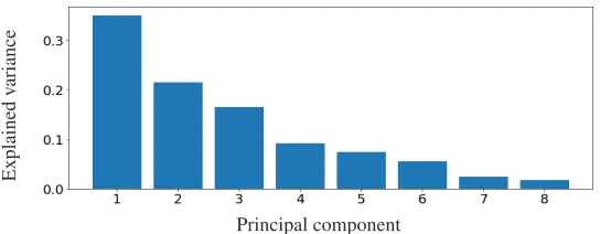
The 10 metrics should represent the state of the server well, but using the whole set as an input for the analytics algorithm would complicate the training without any clear advantage. We, therefore, decided to pre-process the data first before performing the analysis. First, the met-rics are each scaled to zero mean and a unit variance, then principal component analysis [8] is used to transform the metrics. Based on observing the variance of the transformed features (see figure 1), only the top 3 dimensions were kept for analysis. This made the input data set for the machine learning smaller while retaining most of the information in the data.

Principal component

Explained

variance

Figure 1: Proportions of variance explained by each principal component.

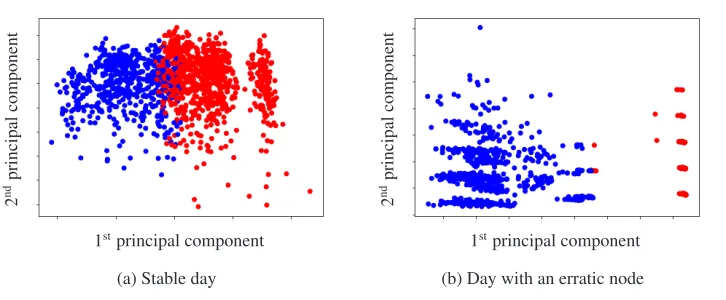
To assess whether there is any useful knowledge to be found, one clusters’1 _{data from} a time period of one day was selected and several clustering algorithms were fitted. Other than basic exploration, clustering can be also used as anomaly detection. For thek-means [9] algorithm, one can measure the distance of the examined data point from the center of the cluster it was assigned to. If the distance exceeds some limit, the point is marked as an anomaly. Moreover, the mixture of gaussians [10] clustering algorithm also computes a per data point probability of each cluster, which can be used as well. The number of clusters was set to two, however, we were expecting all the data points should form only one cluster with several outliers possibly scattered around. In practice, many false positives were observed when this approach was applied on a day with a stable service (see Figure 2a). Conversely, on a day where one of the nodes actually displayed some erratic behavior, its data formed a separate cluster, therefore, it could not be identified using the approaches described above (see Figure 2b).

(4)

1st_{principal component}

2

nd

principal

component

(a) Stable day

2

nd

principal

component

(b) Day with an erratic node

Figure 2: Result of a run of the K-Means clustering algorithm on PCA transformed data.

As an improvement to clustering, we thought of utilizing supervised learning. In our case the input of the learned function would be a vector composed of multiple consecutive state snapshots and the output would be the state snapshot that follows the last one of the input. Using the described pre-processing each state snapshot would consist of 3 elements (when using 3 principal components). Length of history was set to 4 snapshots, which would represent a time window of 80 minutes and result in an input vector with the length of 12. In order to maximally leverage the computational power of the available Spark cluster, only algorithms implemented in the SparkML library [11] were considered. None of the available algorithms support a vector type output, therefore 3 separate models had to be trained, each predicting one of the elements of the target snapshot.

To test this approach, two periods spanning several days were selected from the stored data during which the MONIT kafka cluster was running smoothly. To set a baseline the last input snapshot was used as the target one. For initial code development, the linear regression model was used for its speed and simplicity. Cross-validation with 3 folds then picked the model hyperparameters, the best performing model became the benchmark. Then the same approach was applied to train a random forest model [12], which we expected to surpass the simpler linear regression. The performance difference when applied to data from uneventful days is insignificant (see Table 1).

Algorithm Mean Absolute Error Root Mean Squared Error

Baseline [0.42413, 0.98499, 0.63365] [0.82822, 1.4935, 0.82751]

Linear Regression [0.31381, 0.54954, 0.38082] [0.63477, 1.0125, 0.5222]

Random Forests [0.31074, 0.52945, 0.36028] [0.57685, 0.89128, 0.4903]

Table 1: Algorithm errors when applied on data gather on a day without problems. There are 3 errors, 1 per each model predicting one of the elements of the target vector.

When applying the models to data from a day during which one of the servers experienced an anomaly2_{, the di}_ff_{erence between the prediction error on the data point corresponding to} the beginning of the anomaly and the prediction error on the worse predicted anomaly-free

(5)

2

nd

principal

component

(a) Stable day

2

nd

principal

component

(b) Day with an erratic node

Figure 2: Result of a run of the K-Means clustering algorithm on PCA transformed data.

As an improvement to clustering, we thought of utilizing supervised learning. In our case the input of the learned function would be a vector composed of multiple consecutive state snapshots and the output would be the state snapshot that follows the last one of the input. Using the described pre-processing each state snapshot would consist of 3 elements (when using 3 principal components). Length of history was set to 4 snapshots, which would represent a time window of 80 minutes and result in an input vector with the length of 12. In order to maximally leverage the computational power of the available Spark cluster, only algorithms implemented in the SparkML library [11] were considered. None of the available algorithms support a vector type output, therefore 3 separate models had to be trained, each predicting one of the elements of the target snapshot.

To test this approach, two periods spanning several days were selected from the stored data during which the MONIT kafka cluster was running smoothly. To set a baseline the last input snapshot was used as the target one. For initial code development, the linear regression model was used for its speed and simplicity. Cross-validation with 3 folds then picked the model hyperparameters, the best performing model became the benchmark. Then the same approach was applied to train a random forest model [12], which we expected to surpass the simpler linear regression. The performance difference when applied to data from uneventful days is insignificant (see Table 1).

Algorithm Mean Absolute Error Root Mean Squared Error

Baseline [0.42413, 0.98499, 0.63365] [0.82822, 1.4935, 0.82751]

Linear Regression [0.31381, 0.54954, 0.38082] [0.63477, 1.0125, 0.5222]

Random Forests [0.31074, 0.52945, 0.36028] [0.57685, 0.89128, 0.4903]

Table 1: Algorithm errors when applied on data gather on a day without problems. There are 3 errors, 1 per each model predicting one of the elements of the target vector.

When applying the models to data from a day during which one of the servers experienced an anomaly2_{, the di}_ff_{erence between the prediction error on the data point corresponding to} the beginning of the anomaly and the prediction error on the worse predicted anomaly-free

2_{The kafka service on that server was shut down}

host prediction time error0 error1 error2

monit-kafka-dev-001.cern.ch 15:20 4.389288 1.652980 0.345863

Table 2: Top prediction errors of the linear regression model. Server

monit-kafka-dev-001.cern.ch entered erratic state around 15:10 (hostnames were

changed).

host prediction time error0 error1 error2

monit-kafkax-dev-001.cern.ch 15:20 4.318426 4.124729 4.622074

Table 3: Top prediction errors of the random forest model. Server

monit-kafka-dev-001.cern.ch entered erratic state around 15:10 (hostnames were

changed).

data point was larger for the linear regression model compared to the random forest model (see Table 2 and Table 3). This might indicate that the data are linear in its’ nature and using more complex models does not yield supreme results. Interestingly, unlike the linear regression, the random forest model fails to predict the next state of the server even after it stayed in the erratic state for some time.

During code development, the SWAN platform [13] proved to be very useful enabling us to tweak the code and run it in a Spark cluster from a notebook environment considerably speeding up the whole process.

5 Conclusion and Future Work

We built a data processing pipeline using the MONIT infrastructure consuming, aggregating and saving metrics produced by collectd. We then used samples from this ever-growing dataset to train several machine learning models and applied them to the data. The results suggest that the black-box approach is viable when detecting erratic behavior in dedicated servers running a distributed application.

(6)

References

[1] A. Aimar, A.A. Corman, P. Andrade, S. Belov, J.D. Fernandez, B.G. Bear, M. Georgiou, E. Karavakis, L. Magnoni, R.R. Ballesteros et al., Journal of Physics: Conference Series 898, 092033 (2017)

[2] I. Bird, Annual Review of Nuclear and Particle Science 61, 99 (2011), https://doi.org/10.1146/annurev-nucl-102010-130059

[3] X. Espinal, G. Adde, B. Chan, J. Iven, G.L. Presti, M. Lamanna, L. Mascetti, A. Pace, A. Peters, S. Ponce et al., Journal of Physics: Conference Series513, 042017 (2014) [4] Distributed service for collecting, aggregating and moving log data, "Apache Flume"

[software],https://flume.apache.org/

[5] N. Garg,Apache Kafka(Packt Publishing, 2013), ISBN 1782167935, 9781782167938 [6] M. Zaharia, R.S. Xin, P. Wendell, T. Das, M. Armbrust, A. Dave, X. Meng, J. Rosen,

S. Venkataraman, M.J. Franklin et al., Commun. ACM59, 56 (2016)

[7] F. Forster, System information collection daemon, "collectd" [software], https:// github.com/collectd/collectd

[8] H. Abdi, L.J. Williams, WIREs Comput. Stat.2, 433 (2010)

[9] S. P. Lloyd, IEEE Transactions on Information Theory28, 129 (1982)

[10] W. H. Press, S. A. Teukolsky, W. T. Vetterling, B. P. Flannery, inNumerical recipes (Cambridge University Press, Cambridge, c1996), pp. –, 1st edn., ISBN 0521576083 [11] X. Meng, J. Bradley, B. Yavuz, E. Sparks, S. Venkataraman, D. Liu, J. Freeman, D. Tsai,

M. Amde, S. Owen et al., J. Mach. Learn. Res.17, 1235 (2016) [12] L. Breiman, Mach. Learn.45, 5 (2001)