Spectrally-Accurate Algorithm for Flows in 3-Dimensional Rough Channels

(1)

Scholarship@Western

Electronic Thesis and Dissertation Repository

12-4-2015 12:00 AM

Spectrally-Accurate Algorithm for Flows in 3-Dimensional Rough

Channels

Md Nazmus Sakib

The University of Western Ontario

Supervisor J M Floryan

The University of Western Ontario

Graduate Program in Mechanical and Materials Engineering

A thesis submitted in partial fulfillment of the requirements for the degree in Master of Engineering Science

Follow this and additional works at: https://ir.lib.uwo.ca/etd

Part of the Mechanical Engineering Commons

Recommended Citation Recommended Citation

Sakib, Md Nazmus, "Spectrally-Accurate Algorithm for Flows in 3-Dimensional Rough Channels" (2015). Electronic Thesis and Dissertation Repository. 3366.

https://ir.lib.uwo.ca/etd/3366

This Dissertation/Thesis is brought to you for free and open access by Scholarship@Western. It has been accepted for inclusion in Electronic Thesis and Dissertation Repository by an authorized administrator of

(2)

(Thesis format: Monograph)

by

Md Nazmus Sakib

Graduate Program in Mechanical and Materials Engineering

A thesis submitted in partial fulfillment of the requirements for the degree of

Masters of Engineering Science

The School of Graduate and Postdoctoral Studies The University of Western Ontario

London, Ontario, Canada

(3)

ii

Abstract

In this work a spectrally accurate algorithm has been developed for the simulation of

three-dimensional flows bounded by rough walls. The algorithm is based on the velocity-vorticity

formulation and uses the concept of Immersed Boundary Conditions (IBC) for the

enforcement of the boundary conditions. The flow domain is immersed inside a fixed

computational domain. The geometry of the boundaries is expressed in terms of double

Fourier expansions and boundary conditions enter the algorithm in the form of constraints.

The spatial discretization uses Fourier expansions in the stream-wise and span-wise

directions and Chebyshev expansions in the wall-normal direction. The algorithm can use

either the fixed flow rate constraint or the fixed pressure gradient constraint; a direct

implementation of the former constraint is described. An efficient solver which takes

advantage of the structure of the coefficient matrix has been developed. Taking the advantage

of the reality conditions enhances the efficiency of the solver both in terms of memory and

computational speed. It is demonstrated that the applicability of the algorithm can be

extended to more extreme geometries using the over-determined formulation. Various tests

confirm the spectral accuracy of the algorithm.

Keywords

(4)

iii

Co-Authorship Statement

This dissertation is prepared in monograph format and is based on a manuscript that has been

submitted for publication.

N. Sakib, A. Mohammadi and J. M. Floryan, “Spectrally Accurate Immersed Boundary

Conditions Method for Three-Dimensional Flows”, submitted for publication in the Journal

(5)

iv

Dedication

(6)

v

Acknowledgments

I am grateful to my supervisor Prof. J. M. Floryan for his assistance and encouragement. This

work would not have been possible without his continual support and guidance.

I would like to express my gratitude to the members of my advisory committee, Prof. A. G.

Straatman and Prof. E. Savory for their invaluable suggestions and insightful comments.

I would also like to thank my colleagues Alireza Mohammadi, Hadi Vafadar Moradi,

Mohammad Zakir Hossain, Sahab Zandi, Amirreza Seddighi and Seyed Arman Abtahi for

their friendship, support and motivation. I am particularly indebted to Alireza Mohammadi

for his guidance throughout this whole work.

Finally, I would like to mention that this work has been carried out with support from the

(7)

vi

List of Figures

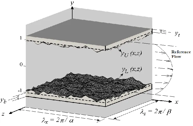
Figure 1: Sketch of the flow and computational domain. ... 6

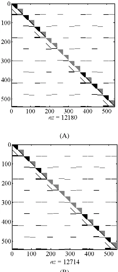
Figure 2: Structure of the coefficient matrix for , For the fixed

pressure gradient constraint (Fig. 2A) ( )( ) and for the fixed flow

rate constraint (Fig. 2B) ( )( ) . The black color identifies the

non-zero elements with giving their total number. The blocks assume various shades of

grey depending on the density of the non-zero elements. ... 33

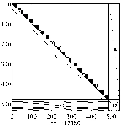
Figure 3: The structure of the re-arranged coefficient matrix for ,

The black color identifies the non-zero elements with giving their total number. The

blocks assume various shades of grey depending on the density of the non-zero elements. .. 35

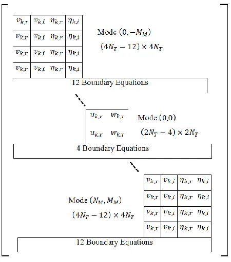
Figure 4: Schematic diagram of the coefficient matrix for the fixed pressure gradient

constraint with all unknowns separated into real and imaginary parts. Each small block

contains coefficients of the unknowns written in the block. ... 37

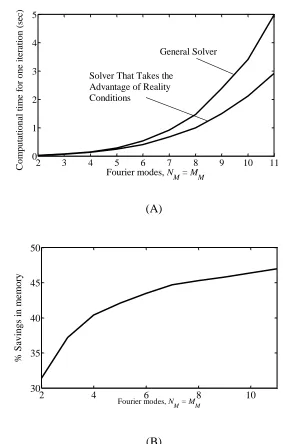
Figure 5: Variations of the computational time per iteration (Fig. 5A) with and without taking

advantage of the complex conjugate property and variations of the memory savings when

taking advantage of the complex conjugate property (Fig. 5B) as functions of the number of

Fourier modes used in the solution. Chebyshev polynomials have been used in the

tests. ... 38

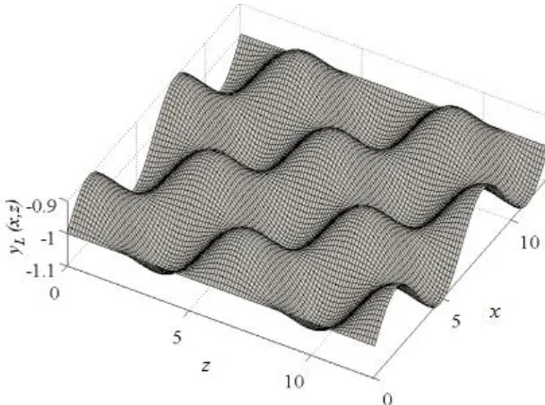
Figure 6: Geometry of the lower wall described by (6.1) with , for two

periods in the x- and z-directions. ... 41

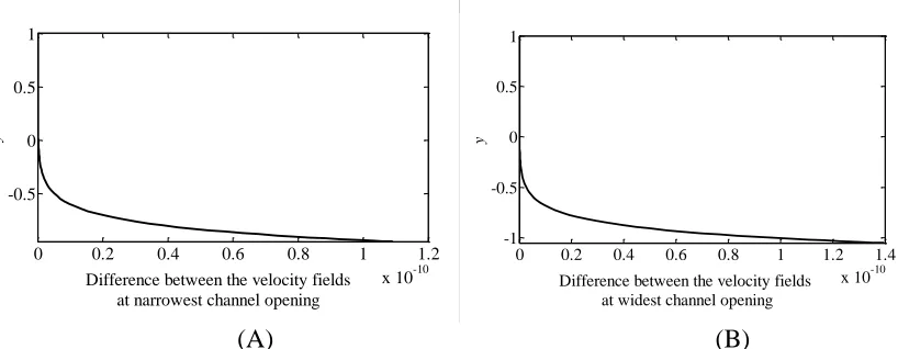
Figure 7: Difference between the velocity fields obtained by current algorithm and algorithm

described by [14] for transverse grooves at narrowest channel opening (Fig.7A) and widest

channel opening (Fig.7B). Calculations have been carried out with and for

(10)

ix

described by [14, 15, 35] for transverse grooves at narrowest channel opening (Fig.8A) and

widest channel opening (Fig.8B). Calculations have been carried out with and

for . ... 42

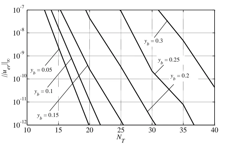
Figure 9: Variation of as a function of the number of Chebyshev polynomials NT

used in the solution. Calculations have been carried out with for the

roughness geometry described by (6.1) with for . ... 44

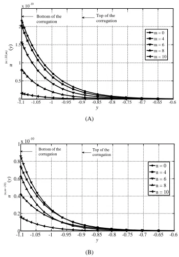
Figure 10: Variation of the modal functions close to the rough boundary. Calculations have

been carried out with for the roughness geometry described by (5.1) ,

for . In Fig. 8A, m changes while n = 10 and in Fig.8B n changes while m =

10. Formation of boundary layers near the rough wall and rapid growth of modal functions

across these layers are clearly visible. ... 45

Figure 11: Variation of the Chebyshev norm of the modal function ( ) as a function of

the Fourier mode index for the roughness geometry described by (6.1) with

for . Computations have been carried out with Fourier modes and

Chebyshev polynomials. ... 46

Figure 12: Variation of ‖ ‖ and ‖ ‖ as a function of the number of Fourier modes

used in the computations for the roughness geometry described by (5.1) with for

Re = 5. Calculations have been carried out using , and (Fig. 10A) and

(Fig. 10B). ... 47

Figure 13: Distributions of the boundary errors ( ) (Fig. 11A), ( ) (Fig.

11B) and ( ) (Fig.11 C) for the roughness geometry described by (5.1) with

for Re = 5 over one period in the x- and z-directions. ... 49

Figure 14: Spectral decomposition of ( ) for the roughness geometry described by

(6.1) with , for Re = 5. Results displayed in Fig. 12A have been obtained

using computational box with , and Fourier modes and those

(11)

x

were used. ... 50

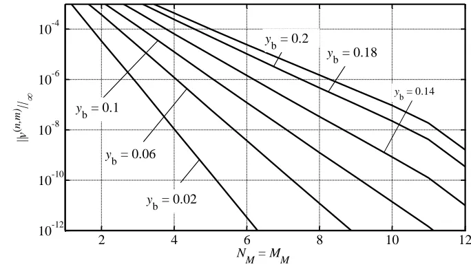
Figure 15: Variations of the error norm ‖ ‖ as a function of the roughness amplitude

(Fig.13 A) and as a function of the roughness wave number with (Fig.13 B) for the

roughness geometry described by (6.1). Calculations have been carried out using

Chebyshev polynomials and (solid lines) and (dash lines)

Fourier modes. ... 51

Figure 16: Variation of the error norm ‖ ‖ as a function of the Reynolds number Re

for the roughness geometry described by (6.1) with and different values of .

Computations have been carried out using Chebyshev polynomials and

Fourier modes. ... 52

Figure 17: Structure of the coefficient matrix for the over-determined formulation with

, and . Black color represents the non-zero

elements with denoting their number. Figure 15A displays the initial form of the matrix

while Fig. 15B shows the form after extractions of the largest diagonal matrix A from H. The

blocks assume various shades of grey depending on the density of the non-zero elements. .. 56

Figure 18: Spectral decomposition of ( ) at the rough wall for the roughness

geometry described by (6.1) with , for Re =10. Computations have

been carried out using Chebyshev polynomials, Fourier modes for

the field equations, and Fourier modes for the boundary conditions. .... 57

Figure 19: Variations of the error norm ‖ ‖ as a function of the roughness amplitude

(Fig.17 A) for the roughness geometry described by (6.1) with for Re = 10 and

as a function of the roughness wave number (Fig.17 B) for the roughness amplitude

= 0.08. Calculations have been carried out using Chebyshev polynomials and

Fourier modes for the field equations. ... 58

(12)

xi

List of Appendices

Appendix A: Analysis of Mode (0,0)... 64

Appendix B: Determination of Chebyshev Expansion Coefficient for a Known Modal

Function ………..65

Appendix C: Evaluation of Fourier expansions representing periodic functions formed by

the values of the Chebyshev polynomials, its derivatives and the reference flow velocity

(13)

xii

List of Abbreviations, Symbols and nomenclature

Abbreviations

IB Immersed boundary

IBC Immersed boundary conditions

RF Relaxation factor

FFT Singular value decomposition

SVD Singular value decomposition

Nomenclatures used in Section 2

( ) Physical coordinate system

, Shape of the upper wall in the physical coordinate system

, Wave numbers in the x- and z-directions

, Wave lengths in x- and z-directions

, Number of Fourier modes used in the x- and z-direction to

describe the roughness geometry

( )

, ( ) Fourier expansion coefficients of the upper and lower wall in the physical coordinate system.

Mean channel opening

Maximum velocity of the reference flow in the direction of total

pressure gradient

Reynolds number

(14)

xiii

⃗ , ⃗ Reference velocity vector and total velocity vector

, , Components of total velocity in the x-, y- and z-directions

Components of reference velocity in the x-, y- and z-directions

Modification velocity components in the x-, y- and z-directions

, , Total pressure, reference pressure and pressure modification

, Mean pressure gradient components in the x- and z-directions

, Modifications of the mean pressure gradient components in the

x- and z-directions

( ) Mean flow rate in the x- and z-directions

, Reference flow rate and flow rate modification in the x-direction

, Reference flow rate and flow rate modification in the z-direction

Mean Pressure gradient in the x-direction

⃗⃗ , ⃗⃗ , ⃗⃗ Vorticity vector for total flow, reference flow and flow

modification

, , Components of total vorticity in the x-, y- and z-directions

Components of modification vorticity in the x-, y- and z

-directions

(15)

xiv

, , Nonlinear terms associated with x-, y- and z-momentum

equations

( ̂ ) Computational coordinate system

Constant for coordinate transformation

, Locations of extremities for the upper and lower wall

̂ , ̂ Shape of the upper and lower wall in the transformed coordinate

system

( )

, ( ) Fourier expansion coefficients of the upper and lower wall in the transformed coordinate system.

( ) ( ) ( )_,

( )

Modal functions for wall-normal vorticity, and the modification

velocity components in the x-, y- and z-directions

Derivative with respect to the transverse direction

〈 〉( )_,_〈 _〉( )

Modal functions of the velocity products

( )

, ( ), ( ),

( )

Chebyshev expansion coefficients of the modal functions

representing the vorticity and velocity components

th Chebyshev polynomial of first kind

Order of Chebyshev polynomials used for discretization of the

(16)

xv

( )( ) ( )( )

Chebyshev expansion coefficients of the modal functions of the

velocity products

Weight function

( ), ( ) Coefficient of Fourier expansions for ( ̂ ( )) and

( ̂ ( ))

( )( ), ( )( ) Coefficients of Fourier expansions for the Chebyshev polynomials at the upper and lower wall.

( )( ), ( )( ) Coefficients of Fourier expansions for the first derivative of the Chebyshev polynomials at the upper and lower wall.

( ) Flow rate in the x-direction

( )

Fourier expansion coefficient of the flow rate in the x-direction

, , Coefficient matrix vector of unknowns and right-hand side

vector

, , , Sections of rearranged coefficient matrix

, Vector of unknowns for the rearranged system of equations

, Right-hand side vectors for the rearranged system of

equations

( )

(17)

xvi ( )

( )

, ( ) , ( )

( )

Imaginary part of the modal functions for wall-normal

vorticity and the three velocity components.

Error norm for the whole physical domain

Error norm for the boundary

( ) Error for whole physical domain

( ) Error at the rough boundary

( ) Computed solution for the whole physical domain

( ) Reference solution for the whole physical domain

( ( ) ) Solution computed at the rough boundary

, Number of Fourier modes used for boundary constraints in

the x- and z-directions for the over-determined formulation

, , Coefficient matrix, vector of unknowns and right-hand side

vector for the over-determined system

, Sections of rearranged coefficient for the over-determined

(18)

xvii

Generalized inverse of

, , Matrices used in QR factorization

, , , Matrices used in SVD method

, , , Sections of the rearranged coefficient matrix

(19)

Section 1

1

Introduction

Roughness can be found in almost every type of flow systems. They have the ability to

enhance or deteriorate the functionality of a flow system. The history of the study of the

effect of surface roughness on fluid flow dates back to the works of Hagen and Darcy [1,

2] who concluded that roughness always increases flow resistance. The quantification of

average drag in terms of friction factor was accomplished by Nikuradse and Moody [3, 4]

who also demonstrated that the drag in laminar flow regime is independent of surface

roughness.

The prevailing belief of surface roughness always increasing drag was first contradicted

by Walsh [5, 6]. His experiments on flows over stream-wise grooves in the form of

riblets demonstrated that surface roughness can reduce turbulent drag. In their works on

drag reducing longitudinal grooves (riblets), Choi, Moin and Kim [7] and Chu and

Karniadakis [8] concluded that though these kinds of grooves have the capability to

reduce turbulent drag, they always increase laminar drag.

The pressure losses for laminar flows over rough surfaces regained the focus because of

the growing interest on the flows in micro-channels and the deviation from the classical

theory found in the works of Papautsky et al, Sobhan and Garimella, Morini, Sharp and

Adrian, and Gamrat et al [9-13]. Mohammadi and Floryan [14] investigated the pressure

losses in grooved channels for laminar flows and found the potential to obtain laminar

drag reducing grooves by proper shaping of the grooves. Mohammadi and Floryan [15]

also studied the drag reducing longitudinal grooves and determined the optimal shape for

such kind of grooves.

The main difficulty associated with the numerical solution of flow problems bounded by

rough walls is modeling the effect of surface roughness. Methods based on the mapping

of the irregular boundary into a rectangular domain can provide very high accuracy.

However, these methods suffer from two main disadvantages. The coefficient matrix

(20)

computational cost [16]. This draw back becomes prominent for unsteady problems as

the coefficient matrix is reconstructed at each time step. Moreover, these algorithms have

limitations in terms of geometry as they cannot handle singularity in the mapping.

The immersed boundary (IB) method provides a general conceptual basis for developing

efficient computational tools to solve flow problems involving complex boundary

geometries. The original concept was proposed by Peskin [17] in the context of cardiac

mechanics problems. The method works by discretizing the governing equations within a

regular computational domain that surrounds the complex flow domain. Special

procedures are then used to enforce the boundary conditions along the physical

boundaries, immersed within the computational domain. The computational efficiency of

this class of methods stems from the elimination of the cost of generating boundary

conforming grids.

The essence of the IB method is to impose forcing at the edge of the computational

domain so that the flow quantities evaluated along the edge of the physical domain

assume values specified by the boundary conditions. Various implementations have been

developed over the past few decades [18, 19] with the forcing applied in either a

continuous or discrete manner. The majority of implementations apply low-order

finite-difference, finite-volume or finite-element techniques for the spatial discretization

[20-22] resulting in limited spatial accuracy. Some recent implementations employ spectral

discretization to improve the solution accuracy although the complete solutions are

nevertheless not spectrally accurate [23, 24].

A fully, spectrally-accurate version of the IB method, referred to as the Immersed

Boundary Conditions (IBC) method was proposed in [25] for two-dimensional flow

problems. The geometry of the physical boundaries is described by Fourier expansions

which limits the applicability of the method to periodic domains. The method is

nevertheless applicable to a very wide class of problems of physical interest. The

discretization relies on two types of Fourier expansions, one for the field variables and

one for the boundary conditions. The boundary relations responsible for the enforcement

(21)

conditions with spectral accuracy. Use of the Chebyshev expansions in the non-periodic

direction makes the algorithm effectively gridless and, thus, allows quick adaptation to

different geometries. The IBC method has been extended to unsteady problems involving

both fixed [16] and time-dependent boundary shapes [26-29]. It has also been extended to

three-dimensional problems described by the Laplace operator [30]. From an application

perspective, the method has been instrumental in the search for drag reducing grooves

[14, 15 and 31] as well as in the analysis of instabilities of shear layers bounded by

grooved surfaces [32-38].

The construction of the boundary relations yields a number of constraints in the IBC

method in excess of what is required to form a closed system of algebraic equations [39].

The “classical” formulation retains enough of these constraints corresponding to the

lowest Fourier modes to form a closed system. Although spatial discretizations using

Fourier and Chebyshev expansions lead to the coveted spectral convergence properties,

the computational cost of the method increases very rapidly with increasing boundary

complexities. This cost may be lowered by using the over-determined formulation where

the number of boundary relations is in excess of the field equations [39]. The cost can

also be lowered by using specialized linear solvers [40, 41].

The above discussion shows that most of the existing efforts, with the exception of [30],

have been focused on two-dimensional problems. There is therefore a need to develop an

extension of the IBC method suitable for the analysis of three-dimensional flows. One

needs to pay attention to the memory and computational cost as both of them increase

rapidly with increased geometric complexity. This is so because the modal equations

resulting from the discretization of the field equation are coupled through boundary

properties, unlike the case of a smooth channel [42].

The present work deals with the development of the three-dimensional version of the IBC

method with applications focused on the analysis of flows in domains bounded by rough

walls. Section 2 introduces the model problem. Section 3 describes the numerical

formulation of the problem. In particular, Section 3.1 discusses the velocity-vorticity

(22)

presents the discretization of the field equations, Section 3.2.2 discusses the discretization

of the boundary conditions and Section 3.2.3 presents the discretization of the flow

constraints. Section 4 is focused on the solution process. In particular, Section 4.1

describes the specialized linear solver used repeatedly during the iterative solution

process while Section 4.2 discusses efficiencies resulting from taking advantage of the

complex conjugate property of the unknowns. Section 5 discusses the evaluation of the

pressure field. Section 6 discusses testing of the algorithm. Section 7 presents the

over-determined formulation of this algorithm and discusses the range of its applicability.

(23)

Section 2

2

Problem Formulation

The mathematical formulation of the problem has been presented in this section. Section

2.1 describes the geometry of flow domain, section 2.2 provides the governing equations,

the reference flow has been introduced in section 2.3 and section 2.4 presents the flow

between rough walls.

2.1 Geometry of the Flow Domain

Consider a channel formed by rough walls extending to in the x- and z-directions.

The upper and lower walls are located at ( ) and ( ), respectively. It is

assumed that the roughness is periodic in the x- and z-directions with wavelengths

and where and stand for the wave numbers in the x- and z

-directions, respectively (Figure 1). The channel geometry can be described using Fourier

expansions of the form

( ) ∑ ∑ ( ) ( )

(2.1a)

( ) ∑ ∑ ( ) ( )

(2.1b)

where half of the mean channel opening has been used as the length scale

and and denote the number of Fourier modes required for the description of the

roughness geometry in the x- and z-directions. The expansion coefficients satisfy the

reality conditions of the form ( ) ( ) , ( ) ( ) , ( )

( )

and ( ) ( ) where star denotes the complex conjugates. As we

are interested in the effect of flow modulations, we assume that the mean openings of the

rough channel and the reference smooth channel are the same and, thus,

( )

(24)

Figure 1: Sketch of the flow and computational domain.

2.2 Governing Equations

Flow in the channel is driven by a pressure gradient parallel to the ( )-plane. The

velocity and pressure fields are described by the continuity and Navier-Stokes equations

of the form

⃗ (2.3a)

( ⃗ ) ⃗ ⃗⃗⃗ (2.3b)

where . /, ⃗ ( ) is the velocity vector with , , denoting

components in the x-, y-, and z-directions, respectively, ⃗ .

/, and

p stands for the pressure. In the above, and have been used at the velocity

(25)

discussed in Section 2.3. The Reynolds number is defined as ⁄ where

denotes the kinematic viscosity.

The flow is subject to the no-slip and no-penetration conditions at the walls of the form

⃗ at ( ) and ( ). (2.4)

2.3 Flow in a Smooth Channel

Flow in the smooth channel represents the reference case and the corresponding velocity

and pressure field have the form

⃗ ( ) 0 ( ) ( )1 (2.5a)

(2.5b)

where ⃗ ( , , ) is the reference velocity vector, stands for the reference

pressure and and denote the pressure gradient components in the x- and z

-directions, respectively. The total pressure gradient and its components are related

according to the following relation

√ . (2.6)

As the fluid flows in the direction of the total pressure gradient, one can choose either the

x- or z-axis to coincide with this direction without loss of generality. The velocity scale

is chosen as the maximum of the velocity of the reference flow in the direction of

the total pressure gradient.

2.4 Flow between Rough Walls

We shall represent flow between the rough walls as a sum of the reference flow and flow

(26)

⃗ ( ) ( ( ) ( ) ( ))

( ( ) ( ) ( ) ( ) ( )), (2.7a)

( ) ( ) ( ) ( ) (2.7b)

where subscripts 0 and 1 refer to the reference flow and the flow modification,

respectively, and denote the modifications of the mean pressure gradient in the x-

and z-directions, respectively, and ( ) denotes the periodic part of the pressure

modifications.

Substitution of (2.7) into (2.3) yields the following form of the field equations

(2.8a) . /

. / (2.8b)

. /

. / (2.8c)

. /

. / (2.8d)

The boundary conditions (2.4) can be expressed in the form

( ( )) ( ( )) (2.9a)

( ( )) ( ( )) (2.9b)

( ( )) (2.9c)

(27)

( ( )) ( ( )) (2.9e)

( ( )) ( ( )) (2.9f)

The above system needs two closing conditions. We shall consider either the fixed flow

rate constraint or the fixed pressure gradient constraint in both the x- and z-directions. To

apply the fixed flow rate constraint we assume that the mean flow rates in x- and z

-directions are known. This constraint in the x-direction takes the form of

( ) _⁄ ∫ ⁄ ∫ _{( )}( ) ( )

_⁄ ∫ ⁄ ∫ _{( )}( ), ( ) ( )-

(2.10)

where and are the reference flow rate and the flow rate modification due to

roughness, respectively. can be specified arbitrarily with = 0 implying that the

flow rates in the smooth and rough channels are the same. The flow rate constraint in the

z-direction can be specified in a similar manner and involves and .

The fixed pressure gradient constraints correspond to the specification of the mean

pressure gradients in both the x- and z-directions. The mean pressure gradient in the x

-direction can be expressed as

(2.11)

where and refers to the pressure gradient of the reference flow and the roughness

induced modification, respectively. can be selected arbitrarily with = 0 implying

that flows in the smooth and rough channels are driven by the same pressure gradient.

The pressure gradient constraint in the z-direction can be specified in a similar manner

(28)

Section 3

3

Numerical Solution of the Problem

This section contains the numerical solution of the flow problem. Section 3.1 provides

the suitable form of the governing equations for numerical solution. Section 3.1 deals

with the numerical discretization of the problem where, 3.2.1 presents the discretization

of the field equations, section 3.2.2 discusses the discretization of the boundary

conditions and section 3.2.3 presents the discretization of the fixed flow rate constraint.

3.1 Forms of the Governing Equations Suitable for the

Numerical Solution

We shall use the velocity-vorticity formulation. The vorticity vector is defined as

⃗⃗ ( ) ⃗ . ( ) ( ) ( )/ ⃗⃗ ( ) ⃗⃗ ( ) (3.1)

where

⃗⃗ ( ) (3.2a)

⃗⃗ ( ) . / (3.2b)

In the above, ⃗⃗ stands for the vorticity of the reference flow and ⃗⃗ denotes the vorticity modifications. The field equations can be reduced to a system of two equations for the wall-normal vorticity and velocity components, i.e. for and , in the form of

( ) . / ( ) (3.3a) (3.3b) where (3.4a) .

(29)

( ) ( ) ( ) (3.4c)

( ) ( ) ( ) (3.4d)

( ) ( ) ( ) (3.4e)

The nonlinear terms have been placed on the right hand sides as these terms are

considered known during the iterative solution process. The solution of (3.3) provides

and while and are determined from the continuity equation and the definition of

the wall-normal vorticity by solving the following system

. / , (3.5a)

. / . /. (3.5b)

The appropriate form of the boundary conditions expressed in terms of and will be

presented later in the text.

The above formulation has two limiting cases. Surface roughness in the form of

transverse grooves results in two-dimensional flow modifications. In this case the

vorticity equation (3.3b) is identically satisfied and the wall normal vorticity becomes

zero. The velocity equation (3.3a) reduces to

( ) ( )

.

/ (3.6)

which is equivalent to the equation studied in [42].When the roughness has the form of

longitudinal grooves, the flow modifications are independent of the direction of the

reference flow, the normal and spanwise velocity modifications disappear, the velocity

equation (3.3a) is identically satisfied and the vorticity equation reduces to the form

(30)

which is equivalent to the x-momentum equation simplified for such flow configurations

and studied in [14].

In the present case, the wall-normal velocity and vorticity equations are solved as a

system in both special cases and the properties of the limiting solutions are used for

verification of the consistency of the algorithm.

3.2 Discretization Method

We wish to determine the solution of the flow problem presented in the previous section

with spectral accuracy. We shall use the Immersed Boundary Conditions (IBC) concept

in order to deal with the irregularity of the solution domain. We select a fixed rectangular

computational domain extending over one period in the x- and z-directions and extending

in the y-direction in such a way that the rough boundaries are completely submerged

inside the computational domain and replace the flow boundary conditions with the

equivalent boundary constraints. Figure 1 illustrates the form of the computational

domain. We shall use Chebyshev polynomials for discretization in the transverse

direction and, in order to use their standard definition, the y-extent of the computational

domain needs to be mapped into , -. A mapping of the form

̂ , ( )- (3.8)

is used where ̂ , -, ( ), and and stand for the locations of

extremities of the upper and lower walls (see Fig.1), respectively.

The wall geometries are expressed in the new coordinate system in the form of

̂ ∑ ∑ ( ) ( )_(3.9a)

̂ ∑ ∑ ( ) ( )_(3.9b)

where

( ) ₀ ( )₁

(31)

( ) _{0 (} ₎( )₁ ( ) ( )

for ( ) ( ) (3.10b)

The governing equations transform to the following form

.

̂ / . / .

̂ /

_̂ _̂ (3.11a)

. ̂ /

̂

̂ (3.11b)

where

(3.12a)

.

/ . / (3.12b)

( ) ̂( ) ( ) (3.12c)

( ) ̂( ) ( ) (3.12d)

( ) ̂( ) ( ) (3.12e)

The fixed flow rate constraint in the new coordinate system is expressed as follows

( ) _⁄ ∫ ⁄ ∫_̂ ̂_{( )}( )0 ( ̂) ( ̂ )1 ̂ (3.13)

while the form of the fixed pressure gradient constraint remains unchanged, i.e. it is given

(32)

3.2.1 Discretization of the Field Equations

The unknowns are represented as Fourier expansions in the periodic directions of the

form

( ̂ ) ∑ ∑ ( )_{( ̂)} ( )

∑ ∑ ( )( ̂) ( ) (3.14a)

( ̂ ) ∑ ∑ ( )_{( ̂)} ( )

∑ ∑ ( )( ̂) ( ) (3.14b)

( ̂ ) ∑ ∑ ( )_{( ̂)} ( )

∑ ∑ ( )( ̂) ( ) (3.14c)

( ̂ ) ∑ ∑ ( )_{( ̂)} ( )

∑ ∑ ( )( ̂) ( ) (3.14d)

where and represent truncations in the x- and z-directions, respectively, and

( ) ( ) ( )_, ( )_{are the modal functions for the wall-normal vorticity and}

the streamwise, wall-normal and spanwise velocity components, respectively. The modal

functions satisfy the reality conditions of the form ( ) ( ) ( )

( ) ( ) ( ) ( ) ( ) _, ( )( ) _, ( ) ( ) _, ( ) ( ) _, ( ) ( ) _{where star denotes the complex}

conjugates.

Substitution of (3.14) into (3.11) and separation of Fourier modes lead to a system of

ordinary differential equations for the modal function of the form

0

( ) ( )1 ( )( ̂)

(33)

.

/ ( )( ̂) ( ) ( )( ̂)

( ) (3.15b)

for and where

(3.16a)

(3.16b)

(3.16c)

( ) _[ ( ) ( )_]

( ) (3.16d)

( ) ( ) ( )

(3.16e)

( )_〈 _〉( )_〈 _〉( )_〈 _〉( )_(3.16f)

( )_〈 _〉( )_〈 _〉( )_〈 _〉( )_(3.16g)

( )_〈 _〉( )_〈 _〉( )_〈 _〉( )_(3.16h)

In the above, 〈 〉( ) denotes the Fourier coefficients of the product ( ), i.e.

( ) ∑ ∑ 〈 〉( )_{( ̂)} ( )

. (3.17)

Similar notation is used for the other products, i.e. ( ) ( ) ( ) ( ),

( ). Functions , , , , , which are treated as known during the solution

process, are replaced by their Fourier expansionswith ( ), ( ), ( ), ( ),

( )_{representing the relevant modal functions. Equation (3.15) represents a}

sixth-order sub-system for each modal function and requires six boundary conditions. Solution

of the complete system results in the determination of the modal functions for and .

The modal form of (3.5) provides expressions for the evaluation of the modal function for

(34)

( )_{( ̂)}

[

( )( )_]_{, (3.18a)}

( )_{( ̂)}

[

( )( )_]_{. (3.18b)}

System (3.15) written for n = m = 0 leads to ( ) and ( ) (see Appendix A)

and, thus, it does not provide a basis for the evaluation of both ( ) and ( ). As these

two components contribute to the nonlinear terms, it is necessary to provide other means

for their determination. Here we return to the primitive variables, substitute

(3.14b)-(3.14d) into the x- and z-components of the momentum equation (2.3b) and extract

modes ( ) ( ) to arrive at

( ) 〈 〉( ) (3.19a)

( ) 〈 〉( ) (3.19b)

The above system is fourth-order, requires four boundary conditions and involves two

unknown constants, i.e. and . For the fixed pressure gradient constraints, both and

are specified. For the fixed flow rate constraint, the specified flow rate corrections

and provide conditions required for the determination of and . We shall discuss

the numerical implementation of these conditions later in this presentation.

The solution of the modal equations (3.15) and (3.19) begins with expressing the modal

functions in terms of Chebyshev expansions of the form

( )_{( ̂) ∑} ( ) _{( ̂) ∑} ( ) _{( ̂)}

(3.20a)

( )_{( ̂) ∑} ( ) _{( ̂) ∑} ( ) _{( ̂)}

(3.20b)

( )_{( ̂) ∑} ( ) _{( ̂) ∑} ( ) _{( ̂)}

(3.20c)

( )_{( ̂) ∑} ( ) _{( ̂) ∑} ( ) _{( ̂)}

(35)

where ( ), ( ), ( ) and ( ) are the Chebyshev expansion coefficients for the

modal functions of ( ), ( ), ( )and ( ), denotes the kth-order Chebyshev

polynomial of the first kind and is the number of Chebyshev polynomials retained in

the solution.

Algebraic equations for the Chebyshev expansion coefficients are constructed using the

Galerkin projection method. Equations (3.20) are substituted into (3.15) and (3.19), and

projections of residua onto the base functions are set to zero. This process is explained

using equation (3.15a) as an example and similar processes are used with the remaining

equations.

Substitution of (3.20) into (3.15a) provides the following expression

∑ 0

( )

( ) 1 ( )

[ 〈 〉( ) _〈 _〉( )_]

[( ) 〈 〉( )_〈 _〉( )_{( )} _〈 _〉( )

〈 〉( )] [ 〈 〉( ) 〈 〉( )] (3.21)

where ( ) on the right hand side is written in an explicit manner. All terms on the

right hand side are considered to be known and need to be expressed in terms of

Chebyshev expansions as follows

[〈 〉( )_〈 _〉( )_〈 _〉( )_〈 _〉( )_〈 _〉( )_〈 _〉( )_{]( ̂)}

∑ 0( )( ) ( )( ) ( )( ) ( )( ) ( )( ) ( )( )1 ( ̂)

(3.22)

where ( )( ) ( )( ) ( )( ) ( )( ) ( )( ) ( )( ) are

(36)

the k-th expansion coefficient for the modal function (m,n) of the product (u1u1). These

coefficients need to be recomputed at the beginning of each iteration with the relevant

method described in Appendix B.

Substitution of (3.22) into (3.21) provides the following expression for the residue

function

∑ 0

( )

( ) 1 ( ) ∑ 20 ( )( )

( )( )1 0 ( )( ) ( )( ) ( )( )

( )( )1 0 ( )( ) ( )( )1 3 ( ̂)

(3.23)

Its projections onto the base functions are expressed in terms of the inner product defined

as

〈 ( ̂) ( ̂)〉 ∫_̂ ̂ ( ̂) ( ̂) ( ̂) ̂ (3.24)

where √ ̂⁄ is the weight function. Equation (3.24) can be written explicitly

as

∑ 0〈 〉

〈 〉

〈 〉 〈 〉

〈 〉 〈 〉 〈 〉 〈 〉

〈 〉1 ( ) ∑ 20 ( )( ) ( )( )1〈 〉

0 ( )( ) ( )( ) ( )( ) ( )( )1〈 〉

0 ( )( ) ( )( )1〈 〉3 (3.25a)

where , with ( ) ( ). This process results in

equations for each modal function, however, we shall retain only the first –

(37)

A similar process applied to (3.15b) results in

∑ 0.〈 〉

〈 〉 〈 〉 〈 〉/

( )

( 〈 〉 〈 〉) ( )1

∑ 20 ( )( ) ( )( )1〈 〉 0( )( )( )

( )( ) ( )( )13 (3.25b)

where we retain only – leading equations, and applied to (3.19) leads to

∑

( )_〈 _〉

〈 〉 ∑ ( )( )〈 〉

(3.26a)

∑

( )_〈 _〉

〈 〉 ∑ ( )( )〈 〉

(3.26b)

where we also retain only – of the leading equations. The inner products of the

Chebyshev polynomials found in (3.25)-(3.26) are given analytically in the form of

〈 〉 {

⁄ (3.27)

The inner products involving the derivatives of the Chebyshev polynomials can be

expressed analytically with the help of the following relations

( ̂) , ( ̂) ̂, ( ̂) ̂ ( ̂) ( ̂) (3.28)

( ̂) , ( ̂) , ( ̂) (3.29)

(38)

Evaluation of the inner products involving the reference flow quantities is explained

using 〈 〉 as an example. ( ̂) is expressed in terms of the Chebyshev expansion

of the form

( ̂) ∑ ( ̂), (3.31)

where stands for the expansion coefficients. According to (2.5) and (3.8), ( ̂) can

also be expressed as

( ̂) ( ̂ ̂ ) (3.32)

where, and . Comparison of (3.31) and (3.32) results in

. /,

, . (3.33)

The inner product 〈 〉 can be written as

〈 〉 ∫_̂ ̂ ∑ ̂ ∑ ∫_̂ ̂ ̂ (3.34)

Since a product of two Chebyshev polynomials can be expressed as a sum of the form

( ), (3.35)

(3.34) can be expressed as

〈 〉 ∑ 0∫_̂ ̂ ̂ ∫_̂ ̂ ̂1

∑ [〈 〉 〈 〉] (3.36)

where the inner products of the individual Chebyshev polynomials are expressed by

(3.27). The other inner products involving the reference flow quantities are evaluated in a

(39)

3.2.2 Discretization of the Boundary Conditions

Substitution of (3.14) into (2.9) provides the modal form of the boundary conditions, i.e.

∑ ∑ ( )_{( ̂} _{( ))} ( )

( ̂ ) (3.37a)

∑ ∑ ( )_{( ̂} _{( ))} ( ) ( ̂ ) (3.37b) ∑ ∑ ( )_{( ̂} _{( ))} ( ) (3.37c) ∑ ∑ ( )_{( ̂} _{( ))} ( ) (3.37d) ∑ ∑ ( )_{( ̂} _{( ))} ( )

( ̂ ) (3.37e)

∑ ∑ ( )_{( ̂} _{( ))} ( ) _{( ̂} ₎

(3.37f)

The form of these conditions expressed in terms of and is obtained by substituting

(3.18) into (3.37), i.e.

∑ ∑ [ ( )_{( ̂} _{( ))}( )_{( ̂} _{( ))]} ( ) ( ) ( )

( )( ̂ ( )) ( ̂ ) (3.38a)

∑ ∑ [ ( )_{( ̂} _{( ))}( )_{( ̂} _{( ))]} ( ) ( ) ( )

( )( ̂ ( )) ( ̂ ) (3.38b)

∑ ∑ ( )_{( ̂} _{( ))} ( ) (3.38c) ∑ ∑ ( )_{( ̂} _{( ))} ( ) (3.38d) ∑ ∑ [ ( )_{( ̂} _{( ))}( )_{( ̂} _{( ))]} ( ) ( ) ( )

(40)

∑ ∑ [ ( )_{( ̂} _{( ))}( )_{( ̂} _{( ))]} ( ) ( ) ( )

( )( ̂ ( )) ( ̂ ) (3.38f)

The above relations involve all modal functions due to the irregularity of the rough walls;

they can be separated into boundary conditions for the individual modal functions in the

case of smooth walls.

We shall now discuss the numerical implementation of the above conditions. The

discussion is limited to the condition for u1 at the upper wall as the remaining conditions

can be treated in a similar manner.

Substituting (3.20) into (3.38a) we obtain

∑ ∑ 0∑ ( ) _{( ̂} _{( ))} ( ) ( )

∑ ( ) ( ̂ ( ))1 ( )

∑ ( ) ( ̂ ( )) ( ̂ ( )) (3.39)

Values of Chebyshev polynomials, their first derivative as well as and evaluated at

the rough wall represent periodic functions which can be expressed in terms of Fourier

expansions of the form

( ̂ ( )) ∑ ∑(( ) ) ( )( ) ( )

(( ) ) (( ) )

(( ) ) (3.40a)

( ̂ ( )) ∑ ∑(( ) ) ( )( ) ( )

(( ) ) (( ) )

(( ) ) (3.40b)

(41)

In the above, ( )( ), ( )( ), ( )( ) and ( )( ) are the known Fourier

expansion coefficients for ( ̂ ), ( ̂ ), ( ̂ ) and ( ̂ ), respectively. The

process leading to the evaluation of these coefficients is explained in Appendix C. When

the shape of the rough wall is described using Fourier coefficients in the x-direction,

the Fourier expansion describing values of the Chebyshev polynomial of order ( )

evaluated at this wall involves ( ) terms, which explains the summation limit

in the x-direction in (3.40). Since velocity components of the reference flow are quadratic

functions of ̂ , their values evaluated at the rough wall involve Fourier coefficients.

Similar arguments explain the limits of expansions in the z-direction.

Substitution of (3.40) into (3.39) and separation of Fourier modes result in

∑ ∑ ∑

0

( )_{( )}( )( )_{( )}( )₁ ( ) ( )

∑ ( )( )( ) ( )( ) (3.41)

In the above, , where ( ) and

( ) . Equation (3.41) provides ( )( ) boundary

relations. Their enforcement guarantees the enforcement of the physical boundary

condition at the rough wall. As the discretization of the field equations resulted in only

( )( ) equations, one can either retain only the leading (

)( ) of the boundary relations or enforce more boundary relations resulting in

the over-determined system.

The final form of all boundary relations can be written as follows

∑ ∑ ∑

0

( )_{( )}( )( )_{( )}( )₁ ( ) ( )

∑ ( )( )( ) ( )( ) (3.42a)

∑ ∑ ∑

0

(42)

∑ ( )( )( ) ( )( ) (3.42b)

∑ ∑ ∑ ( )( )( ) (3.42c)

∑ ∑ ∑ ( )( )( ) (3.42d)

∑ ∑ ∑

0

( )_{( )}( )( )_{( )}( )₁

( ) ( )

∑ ( )( )( ) ( )( ) (3.42e)

∑ ∑ ∑

0

( )_{( )}( )( )_{( )}( )₁

( ) ( )

∑ ( )( )( ) ( )( ) (3.42f)

where , The reader may note that boundary relations

for ( ) ( ) come naturally from (3.42a)-(3.42b) and (3.42e)-(3.42f).

3.2.3 Discretization of the Flow Rate Constraint

In the case of the fixed pressure gradient constraints, and in (3.19) are known and

the discretization process is complete. In the case of the fixed flow rate constraints, one

needs to discretize these constraints in order to construct conditions required for the

determination of and . We shall now discuss the discretization of the flow rate

constraint in the x-direction as discretization in the z-direction follows the same path.

The flow rate in the x-direction can be expressed as

( ) _⁄ ∫ ⁄ ∫ _{( )}( ) ( )

_⁄ ∫ ⁄ ∫ _{( )}( ), ( ) ( )-

(43)

_⁄ ( ) _⁄ ( ) (3.43)

The first integral on the right had side of (3.43) involves only the reference flow

quantities and can be evaluated as follows

( ) ∫ ⁄ ( )

∫ ⁄ ∫ _{( )}( )( )

∫ ⁄ 0 ( ) ( ) ( ) ( )1 (3.44)

where

̂ , , . (3.45)

Substituting (3.45) into (3.44) results in

( ) ∫ ⁄ [ ⁄ ( ̂ ( ) ̂ ( )) ( ̂ ( ) ̂ ( ))

( )( ̂ ( ) ̂ ( ))] (3.46)

to be followed by expressing ̂, ̂ and ̂ in terms of Chebyshev polynomials, i.e.

̂ ( ̂), ̂ ( ( ̂) ( ̂)) ⁄ , ̂ ( ( ̂) ( ̂)) ⁄ . (3.47)

The resulting expression has the form of

( ) ∫ 0∑ ∑ 2 ⁄ .( )( ) ( )( )/

⁄

.( )⁄ ( ) ( )( )/ ( ⁄ ( )).( )( ) ( )( )/ .( )( ) ( )( )/3 ₁_(3.48)

where advantage has been taken of (3.40a) and ( ) and

( ) . Since

(44)

the final expression for ( ) has the following form

( ) . / ∑ 2 ⁄ .( )( ) ( )( )/

.( )⁄ ( ) ( )( )/ ( ⁄ ( )).( )( ) ( )( )/

.( )( ) ( )( )/3 _{. (3.50)}

The evaluation of the second integral begins by using in discretized form and

expressing its modal functions in terms of the wall-normal velocity and vorticity for all

modes except mode ( ). This process leads to

∫ ⁄ ∫ _{( )}( ) ( ) _∫ _∫ ̂ ( ) _{( ̂ ) ̂} ̂ ( ) ⁄ ∫ ⁄ ∫_̂ ̂_{( )}( )∑ ( ) ( ̂) ̂ ∫ ∫ ∑ ∑ ∑ 0 ( ) _{( ̂)} ( ) ( ) ̂ ( ) ̂ ( ) ⁄

( ) ( ̂)1 ( )_̂

_∑ ₂( )_∫ ⁄ _{( )}₃

_∑ _∑ _∑ ₂

.

( ) _{/ ∫} ⁄ _{( )} ₃ ( ) ( )

_∑ _∑ _∑ ₂

.

( ) _{/ ∫} ⁄ _{( )} ₃ ( ) ( ) ,(3.51) where

( ) 0∫_̂ ̂_{( )}( ) ( ̂) ̂1, (3.52a)

( ) 0∫_̂ ̂_{( )}( ) ( ̂) ̂1 ( ̂ ) ( ̂ ). (3.52b)

The analytical evaluation of the integral ( ) results in

(45)

( ) 0 ( ̂ ) ( ̂ )

( ̂ ) ( ̂ )

1, . (3.53b)

Since the geometry is periodic, functions formed by values of the Chebyshev

polynomials evaluated at the upper wall are periodic and, thus, one can write expressions

for ( ) and ( ), with the help of (3.40a) in the form of

( ) ∑ ∑ ( ) ( )

, (3.54a)

( ) ∑ ∑ ( ) ( )

, (3.54b)

where

( ) _{( )}( )_{( )}( )

, ( ) .( )( ) ( )( )/ (3.55a)

( ) _[( ) ( ) ( ) ( )

( )( ) ( )( )

], , (3.55b)

( ) _{( )}( )_{( )}( )

. (3.56)

Substituting (3.54) into (3.51) results in

( ) ∑ ∑ ∑ 2 ( ) ( ) ∫ ⁄ 3

_∑ _∑ _∑ _∑ _∑ ₂

( ) ( ) ( ) _∫ ⁄ ( ) ₃ ( ) ( )

_∑ _∑ _∑ _∑ _∑ ₂

( ) ( ) ( ) _∫ ⁄ ( ) ₃ ( ) ( ) (3.57) Since ∫ ⁄ ( ) {

, (3.58)

(46)

( ) 2∑ ∑ ( ) ( ) ∑ ∑ ∑ ∑ ( ) ( ) ( ) ( ) ( ) ( )

( ) _}_{, (3.59)}

Re-naming the indices results in

( ) 2∑ ∑ ( )

( ) ∑ ∑ ∑ ∑ ( ) ( ) ( ) ( ) ( ) ( )

_}_(3.60)

where .

Substituting the expressions for ( ) and ( ) into (3.43) and replacing the index m

with q results in the discretized expression for the flow rate of the form

( ) . / ∑ 2 ⁄ .( )( ) ( )( )/

.( )⁄ ( ) ( )( )/ ( ⁄ ( )).( )( ) ( )( )/

.( )( ) ( )( )/3

2∑ ∑ ( ) ( )

∑ ∑ ∑ ∑ ( ) ( )( ) ( ) ( ) ( )

_}_(3.61)

which demonstrates that the flow rate is a periodic function of x. This expression can be

written in a simpler form of

( ) ∑ ( )

(47)

In the case of the fixed volume flow rate constraint, mode zero of the above expression

represents the mean flow and has to be specified. The mean flow rate has two

components, i.e.

( )

(3.63)

where stands for the flow rate of the reference flow and represents the flow rate

modification due to the presence of the roughness. Extracting mode zero from (3.61)

results in

( )

. / 2 ⁄ .( )( ) ( )( )/

.( )⁄ ( ) ( )( )/ ( ⁄ ( )).( )( ) ( )( )/

.( )( ) ( )( )/3

{∑ ( ) ( ) ∑ ∑ ∑ ( ) ( ) ( ) ( ) ( ) ( )

} (3.64)

Substitution of (3.64) into (3.63) results in the following form of the flow rate constraint

∑ ∑ ∑ ( ) ( ) ( ) ( ) ( ) ( ) ∑ ( ) ( )

₂ _⁄_{.( )}( )_{( )}( )_/

.( )⁄ ( ) ( )( )/ ( ⁄ ( )).( )( ) ( )( )/

.( )( ) ( )( )/3 = (3.65)

where all unknowns are on the left hand side. A similar procedure applied to the fixed

flow rate constraint in the z-direction results in

∑ ∑ ∑ ( ) ( ) ( )( ) ( ) ( ) ∑ ( ) ( )

₂ _⁄_{.( )}( )_{( )}( )_/

(48)

.( )⁄ ( ) ( )( )/ ( ⁄ ( )).( )( ) ( )( )/

(49)

Section 4

4

Solution Process

The system (3.25) - (3.26) together with the boundary relations (3.42) and the flow rate

constraints (3.65) - (3.66) represents a coupled nonlinear system of algebraic equations.

This system is solved using the first-order fixed-point iterative method whose details are

described later in this Section. The solution results in the determination of the Chebyshev

expansion coefficients of the wall normal velocity, the wall normal vorticity, modes (0, 0)

for u1 and w1 as well as the pressure gradient corrections in the case of the fixed flow rate

constraints. The remaining modal functions for u1 and w1 are evaluated using (3.19).

Considering that all the nonlinear terms are placed at the right hand side and are treated

as known, one needs to solve a linear system at each iteration step and, subsequently,

determine the new approximation for the nonlinear terms. The process of constructing

the new approximation for the unknowns can be summarized as follows

* + _{* +} _{[* +}( )_{* +} _]_(4.1)

where X is the vector of unknowns, the superscripts j and j+1 identify the current and

next approximations, and the superscript denotes the solution computed at the new

iteration. The iteration process is controlled using the under-relaxation parameter .

At each iteration step, the nonlinear terms are computed using the information available

from the previous iteration. These terms involve velocity products (i.e. , , ….)

which are evaluated in the physical space on a grid involving Chebyshev points in the ̂-

direction and a uniformly distributed grid in the x- and z-directions. The modal functions

for these velocity products (i.e. 〈 〉( ), 〈 〉( ),…) are computed using

two-dimensional Fast Fourier Transform (FFT) for each Chebyshev point using the 3/2 rule to

Spectrally-Accurate Algorithm for Flows in 3-Dimensional Rough Channels

Scholarship@Western

Scholarship@Western

Spectrally-Accurate Algorithm for Flows in 3-Dimensional Rough

Spectrally-Accurate Algorithm for Flows in 3-Dimensional Rough

Channels

Channels

Abstract

Keywords

Co-Authorship Statement

Dedication

Acknowledgments

Table of Contents

List of Figures

List of Appendices

List of Abbreviations, Symbols and nomenclature

Section 1

1

Introduction

Section 2

2

Problem Formulation

2.1

Geometry of the Flow Domain

2.2

Governing Equations

2.3

Flow in a Smooth Channel

2.4

Flow between Rough Walls

Section 3

3

Numerical Solution of the Problem

3.1

Forms of the Governing Equations Suitable for the

Numerical Solution

3.2

Discretization Method

3.2.1

Discretization of the Field Equations

3.2.2

Discretization of the Boundary Conditions

3.2.3

Discretization of the Flow Rate Constraint

Section 4

4

Solution Process