Article
Multiple Tensor Train approximation of parametric
constitutive equations in elasto-viscoplasticity
Clément Olivier1,2,‡, David Ryckelynck1,∗,‡, Julien Cortial2,‡
1
2 3 4
5 6 7 8
9
1 SafranTech,RuedesJeunesBois,Chateaufort,CS80112,78772Magny-Les-Hameaux,France;
2 MINESParisTech,PSL-ResearchUniversity,Centredesmatériaux,CNRSUMR7633,10rueDesbruères,
91003Evry,France;[email protected],[email protected] * Correspondence:[email protected]
Abstract: This work presents a novel approach to construct surrogate models of parametric DifferentialAlgebraicEquationsbasedonatensorrepresentationofthesolutions. Theprocedure consistsinbuildingsimultaneously,foreveryoutputofthereferencemodel,anapproximationgiven intensor-trainformat.Aparsimoniousexplorationoftheparameterspacecoupledwithacompact datarepresentationallowstoalleviatethecurseofdimensionality.Theapproachisthusappropriate whenmanyparameterswithlargedomainsofvariationareinvolved.Thenumericalresultsobtained foranonlinearelasto-viscoplasticconstitutivelawshow thattheconstructedsurrogatemodelis sufficientlyaccuratetoenableparametricstudiessuchasthecalibrationofmaterialcoefficients.
Keywords: parameter-dependentmodel;surrogatemodeling;tensor-traindecomposition;gappy POD;heterogeneousdata;elasto-viscoplasticity
10
1. Introduction
11
Predictive numerical simulations in solid mechanics require complex material laws that involve
12
systems of highly nonlinear Differential Algebraic Equations (DAEs). These models are essential in
13
challenging industrial applications, for instance to study the effects of the extreme thermo-mechanical
14
loadings that turbine blades may sustain in helicopter engines [1] and [2].
15
These DAE systems are referred to as constitutive laws in the material science community. They
16
express, for a specific material, the relationship between the mechanical quantities such as the strain,
17
the stress and miscellaneous internal variables, and stand as the closure relations of the physical
18
equations of mechanics. Complex constitutive equations are often tuned through a set of parameters
19
called material coefficients.
20
An appropriate calibration of these coefficients is necessary to ensure that the numerical model
21
mimics the actual physical behavior. Numerical parametric studies, consisting in analyzing the
22
influence of the parameter values on the solutions, are typically used to perform the identification.
23
However, when the number of parameters increases and unless the computational effort required
24
for a single numerical simulation is negligible, the exploration of the parameter domain turns into a
25
tedious task and exhaustive analyses become unfeasible. Moreover, defining an unambiguous criterion
26
measuring the fidelity of the model to experimental data is a challenge for models with complex
27
behaviors.
28
A common technique to mitigate the aforementioned challenges is to build surrogate models (or
29
metamodels) mapping points of a given parameter space (considered as the inputs of the model) to
30
the outputs of interest of the model. The real-time prediction of DAE solutions for arbitrary parameter
31
values, enabled by the surrogate model, helps the comprehension of constitutive laws and facilitate
32
the conduct of parametric studies. In particular, the robustness of the calibration process can be
33
dramatically improved using surrogate model approaches.
34
The idea of representing the set of all possible parameter-dependent solutions of ODEs and PDEs
35
as a multiway tensor was pioneered with the introduction of the Proper Generalized Decomposition
36
(PGD) [3–5]. In this representation, each dimension corresponds to a spatial/temporal coordinate
37
or a parameter coefficient. The resulting tensor is never assembled explicitly but instead remains an
38
abstract object for which a low-rank approximation based on a Canonical Polyadic decomposition
39
[6] is computed. The PGD method further alleviates the curse of dimensionality by introducing a
40
multidimensional weak formulation over the entire parameter space, and the solutions are sought
41
in a particular form where all variables are separated. When differential operators admit a tensor
42
decomposition, the PGD method is very efficient because the multiple integrals involved in the
43
multidimensional weak form of the equations can be rewritten as a sum of products of simple integrals.
44
Unfortunately realistic constitutive equations or even less sophisticated elasto-viscoplastic models
45
admit no tensor decomposition with respect to the material coefficients and the time variables. An
46
extension of the PGD to highly nonlinear laws is therefore non-trivial. However, many other tensor
47
decomposition approaches have been successfully proposed to approximate functions or solutions of
48
differential equations defined over high dimensional spaces. We refer the reader to [7–9] for detailed
49
reviews on tensor decomposition techniques and their applications.
50
Among the existing formats – CP decomposition [6,10,11], Tucker decomposition [8,12],
51
Hierarchical Tucker decomposition [8,13] – this work investigates the tensor-train (TT) decomposition
52
[14,15]. The TT-cross algorithm, introduced in [14] and further developed in [16,17], is a sampling
53
procedure to build an approximation of a given tensor under the tensor-train format. Sampling
54
procedures in parameter space have proven their ability to reduce nonlinear and non-separable DAEs
55
by using the Proper Orthogonal Decomposition (POD) [18], the Gappy POD [19], or the Empirical
56
Interpolation Method (EIM) [20,21]. These last methods are very convenient when the solutions have
57
only two variables, hence they are considered as second order tensors.
58
This paper aims to extend the sampling procedure of the TT-cross method to DAEs having
59
heterogenous and time-dependent outputs. A common sampling of the parameter space is proposed,
60
though several TT-cross approximations are computed to cope with heterogeneous outputs. These
61
outputs can be scalars, vectors or tensors, with various physical units. In the proposed algorithm,
62
sampling points are not specific to any output although parameters do not affect equally each DAE
63
output. The proposed method is named multiple TT-cross approximation. Similarly to the construction
64
of a reduced integration domain for the hyperreduction of partial differential equations [22] or for
65
the GNAT method [23], the set of sampling points is the union of contributions from the various
66
outputs of the DEA. In this paper, the multiple TT-cross incorporates the Gappy POD method and the
67
developments are focused on the numerical outputs obtained through a numerical integration scheme
68
applied to the DAE.
69
2. Materials and Methods
70
The parametized material model generates several time-dependent quantities of interest (QoI).
71
These quantities can be scalar-, vector- or even tensor-valued (e.g. stress) and are generally of distinct
72
natures, namely expressed with different physical units and/or have different magnitudes. Therefore,
73
the generated data will be segregated according to the QoI it relates to. It will also be structured in a
74
tensor-like fashion to make it amenable to the numerical methods presented in this paper.
75
For a givenχ = 1, . . . ,Ndenoting an arbitrary QoI, the tensor of order d,Aχ ∈ Rn1×···×n
χ
d
(denoted with bold calligraphic letter) refers to a multidimensional array (also called multiway array). Each element ofAχidentified by the indices(i
1, . . .id)∈D1× · · · ×Dd−1×Ddχis denoted by: Aχ(i
whereDk = [1 :nk]fork<d, is the set of natural numbers from 1 tonk(inclusive) andDdχ= [1 :n χ d].
76
The last index is specific to each Aχ, while the other are common to all tensors for
χ = 1, ...,N.
77
Hence, a common sampling of the parameter space D1×. . .×Dd−1can be achieved. The vector
78
Aχ(i
1, . . . ,id−1, :) ∈ Rn
χ
d contains all the components of outputχ at all time instants used for the
79
numerical solution of the DAE and for a given point in the parameter space.
80
Theqthmatricization ofAχdenoted byhAχi
qconsists in dividing the dimensions ofAχinto two groups, theqleading dimensions and the(d−q)trailing dimensions, such that the newly defined multi-indices enumerate respectively the rows and columns of the matrixhAχi
q. For instance, the elements ofhAχi
1andhAχi2are given by:
hAχi
1(i1, j?) =Aχ(i1, . . . ,id)
hAχi
2(i1+ (i2−1)n1,j??) =Aχ(i1, . . . ,id)
wherej?enumerates the multiple indices(i2, . . . ,id)andj??enumerates(i3, . . . ,id). Here again, these matricizations are purely formal because of the curse of dimensionality. In particular, the number of columns inhAχi
1is equal ton2. . .nd−1nχd. The Frobenius norm is denoted byk.kwithout the usual subscriptF. ForAχ∈
Rn1×...n
χ
d, it reads:
kAχk=s
∑
i1,...,id∈D1×···×Dd−1×Ddχ Aχ(i
1, . . . ,id)2
The Frobenius norm of a tensor is invariant under all matricizations of a given tensor.
81
In [14], the Singular Value Decomposition (SVD) is considered in the algorithm called TT-SVD.
82
Because of the curse of dimensionality, the TT-SVD has no practical use, even if tensors have a low
83
rank. More convenient approaches, aim to sample the entries of tensors.
84
For instance, in the snapshot proper orthogonal decomposition (POD) [18], the sampling
85
procedure aims to estimate the rank and an orthogonal reduced basis for the approximation of a
86
matrix A. The method consists in applying the truncated SVD on the submatrix ˜A = A(:,Jpod)
87
constituted by a selection of columnsJpodofA. Hence the accuracy of the resulting POD reduced
88
basis relies on the quality of the sampling procedure that generally introduces a sampling error. This
89
sampling procedure seams to be convenient when considering the first matricizationshAχi qif the
90
productn1n2. . .nqand Card(Jpod)are reasonably small regarding the available computing ressources.
91
But, for large values ofq, the curse of dimensionality makes the snapshot POD alone, intractable.
92
A more practical approach to effectively construct an approximate TT decomposition, called the TT-cross method, is proposed in [14]. The TT-cross consists in dropping the concept of a POD basis and using the Pseudo-Skeleton Decomposition (PSD) introduced in [24] as low-rank approximation. Unlike the TT-SVD, the TT-cross enables to build an approximation based on a sparse exploration of a reference tensor. The Pseudo-Skeleton Decomposition can be used to approximate any matrix A∈Rn×mand is written as:
A=A(:,Jpsd)hA(Ipsd,Jpsd)i−1A(Ipsd, :)
| {z }
=Tpsd
+Epsd (1)
where the setsIpsdandJpsdare respectively a selection of row and column indices. The definition
93
is valid only when the matrixA(Ipsd,Jpsd)is non-singular. In particular, the numbersof rows and
94
columns has to be identical.
This approximation (1) features an interpolation property at the selected rows and columns:
Tpsd(Ipsd, :) =A(Ipsd, :) and Tpsd(:,Jpsd) =A(:,Jpsd) (2) The Pseudo-Skeleton Decomposition is a matrix factorization similar to the decomposition used
96
in the Adaptive Cross Approximation (ACA) [25] and the CUR decomposition [26,27]. Additionally,
97
these references provide algorithms to effectively build the factorization. That decomposition has also
98
been used in the context of model order reduction, for instance in the Empirical Interpolation Method
99
(EIM) proposed in [20,21].
100
The condition thatA(Ipsd,Jpsd)must be non-singular make difficult to share sampling points for
101
various matriceshAχi
qwithχ=1, . . . ,Nhaving their own rank.
102
The Gappy POD introduced in [19] aims at relaxing the aforementioned constraint by combining
103
beneficial features of the Snapshot POD and the Pseudo-Skeleton Decomposition. Indeed, the Gappy
104
POD a) relies on a POD basis that remains computationally affordable, b) requires only a limited
105
number of rows of the matrix to be approximated and c) enables to reuse the set of selected rows for
106
different matrices. These properties are key ingredients for an efficient, parsimonious exploration of
107
the reference tensors. The Gappy POD approximationTgapof a matrixA∈Rn×mis given by:
108
A=V[V(Igap, :)]†A(Igap, :)
| {z }
=Tgap
+Egap (3)
where † denotes the Moore-Penrose pseudo-inverse [28],Igapis a row selection ofsrows and where V∈Rn×ris a POD basis matrix of rankrsuch that :
A(:,Jpod) =V S WT+Epod (4)
In the sequel, because the simulation data inAχare outputs of a DAE system, it does not make
109
sense to sample the last indexid during column sampling ofhAχiq. Each numerical solution of
110
the DAE system generates all the last components of each tensorAχ. Hence, the column sampling
111
is restricted to indicesiq+1, . . .id−1and is replicated for all values ofidinDχd. This special column
112
sampling is denoted byJχ
pod. It is performed randomly by using a low-discrepancy Halton sequence
113
[29].
114
The matrixV(Igap, :)must have linearly independent columns to ensure that the approximation
115
is meaningful. SinceVis a rank-rPOD basis, there exists a set ofsrows such that this property holds
116
as long ass ≥ r. Here,Igapcontains at least the interpolation indices related toV. This latter set
117
is denoted byIχ, such thatV(Iχ, :)is invertible. In the numerical results presented hereafterIχ
118
is the obtained using the Q-DEIM algorithm [30] that was shown to be a superior alternative to the
119
better-known DEIM procedure [31, Algorithm 1].
120
Unlike the PSD, the Gappy POD enables to select a number of rows that exceeds the rank of the low-rank approximation:
Igap=I1 ∪ . . . ∪ IN (5)
This make possible to share sampling points between matrices having their own rank. In this case, the
121
interpolation property does not hold as in the PSD case (2).
122
tensorT ∈Rn1×···×nd is said to be in tensor-train format (TT format) if its elements are given by the
following matrix products:
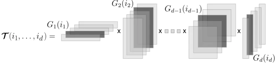
T(i1, . . . ,id) =G1(i1). . .Gd(id)∈R (6) where the so-calledtensor carriages(orcore tensors) are such that fork=1, . . . ,d,:
Gk(ik)∈Rrk−1×rk ∀i k∈ Dk
In the original definition of the tensor-train format [14], the leading and trailing factors
123
(corresponding to G1(i1)andGd(id)for any choice of i1 andid) are respectively row and column
124
vectors. Here, the conventionr0=rd=1 is adopted so that row matricesG1(i1)and column matrices
125
Gd(id)can be interpreted as vectors or matrices depending on the context.
126
The TT format allows significant gains in terms of memory storage and therefore is well-suited
127
to high order tensors. The storage complexity isO(nr¯2d)where ¯r=max(r1, . . . ,rd−1)and depends
128
linearly on the orderdof the tensor. In many applications of practical interest the small TT-ranksrk
129
enable to alleviate the curse of dimensionality [14].
130
The sequential computational complexity of the evaluation of a single element of a tensor in TT
131
format isO dr¯2
. Assuming that ¯ris small enough, the low computational cost allows a real-time
132
evaluation of the underlying tensor. Therefore, in terms of online exploitation, this representation
133
conforms with the expected requirements of the surrogate model. Figure1illustrates the sequence of
134
matrix multiplications required to compute one element of the tensor train.
135
x
x
x
x
Figure 1.Illustration of the evaluation of one element of the tensor train. The entryT(i1, . . . ,id)∈Ris obtained by multiplying the set of matricesG1(i1),G2(i2). . . ,Gd(id)identified by a darker shade.
The objective of the proposed approach is to build for each physics-based tensor Aχ an
136
approximate tensor Tχ given in TT format by using a nested row sampling of the simulation
137
data. Algorithm1provides the set of matrices{Gχ
1, . . . ,G
χ
d}that enable to define the tensor-train
138
decompositions and aggregate sets for row sampling. It is a sequential algorithm that navigates from
139
dimension 1 to dimensiond−1 of tensorsAχ.
140
The method provided by Algorithm1is non-intrusive and relies on the numerical solutions of
141
the DAEs in a black-box fashion.
142
At each iterationk= 1, . . . ,d−1, the Snapshot POD method, used to build the POD reduced
143
basis (9), requires to sample a setJχ
k . The column sampling amounts to a parsimonious selection of
144
˜
nkpoints in the partial discretized parameter domainDk+1× · · · × Dd−1and an exhaustive sampling
145
of the last dimension for each tensorAχ. The considered submatrices ˜Aχ k = A
χ k :,J
χ k
are then
146
constituted of ˜nχ k =n˜kn
χ
d columns (See Figure2).
147
In the row sampling step, specific sets of interpolant rowsIχ
k are first determined independently
148
for each outputχbut a common, aggregated setIk(10) is then used to sample the entries of all outputs.
149
Indeed, computing the elements of all submatricesAχ
k(Ik, :)requiresmkcalls to the DAE system solver
150
with: mk =Card(Ik−1)n˜kwithI0= D1. Furthermore, the Gappy POD naturally accommodates a
Algorithm 1:Multiple TT decomposition
Input: TensorsAχ∈
Rn1×···×nd−1×n
χ
d forχ=1, . . . ,Nassociated with a DAE system Output: Sets of matrices
G1χ, . . . ,Gdχ forχ=1, . . . ,N.
Initialization:
For eachχ, define the matrixA1χ∈R(s0n1)×(n2...nd−1n
χ
d)withs0=1, as the first matricization of
the tensorAχ:
Aχ
1 =hAχi1 (7)
Fork=1, . . . ,d−1do Snapshot POD:
Define consistent sets of sampling columnsJχ
k and evaluate the DAE to fill the matrices ˜
Aχk defined as:
˜
Aχk =Aχk :,Jχ k
for χ=1, . . . ,N
Apply the truncated SVD (4) on each ˜Aχ
k with the truncation toleranceeto get the rank-r χ k matrices:
˜
Aχk =VkχSχk WkχT+Eχpod k with E
χ pod k
≤e
A˜χk
(8)
Vχ
k ∈R(sk−1nk)
×rχ
k for χ=1, . . . ,N (9) Row Sampling:
From eachχ, select a set of rowsIkχapplying the Q-DEIM algorithm [30] to the basisVkχ.
Define the union of all selected rows and the corresponding row selection matrix:
Ik = N [
χ=1
Iχ
k (10)
and
sk=Card(Ik) (11)
Output definitions:
Compute the matricesGχk ∈R(sk−1nk)×sk such that:
Gχk =Vkχ
Vkχ(Ik, :) †
Tensorization:
Define, formally, the tensorsAχ,(k+1)∈
Rsk×nk+1×···×nd−1×n
χ
d such that:
D
Aχ,(k+1)E
1=A
χ
k(Ik, :)∈Rsk×(nk+1...nd−1n
χ
d) (12)
Matricization:
Define, formally, the matrixAχ k+1∈R
(sknk+1)×(nk+2...nd−1nχd)as the second matricization of
the tensorAχ,(k+1):
Aχ k+1=
D
Aχ,(k+1)E
2 (13)
Finalization:
For eachχ=1, . . . ,Nχ, define the matrixGdχ∈R(sd−1n
χ
d)×sd withs
d=1 such that: Gχ
d = A χ
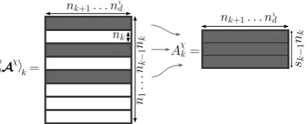
Figure 2.Definition of the submatrix ˜Aχ
k used to construct the POD reduced basis. In the illustration,
the Snapshot POD sample size is ˜nk=3.
number of rows larger than the rankrχ
k for each approximation ofA χ
k, and considering a larger sample
152
size for each individualχis expected to provide a more accurate approximation.
153
The tensorization and matricization steps are purely formal. No call to the DAE system solver is
154
done here. They define the way the simulation data must be ordered in matrices to be approximated
155
at the next iteration. The recursive definition of the matrixAχ
k implies that the latter is equal to the
156
kth matricization of a subtensor extracted fromAχ. Equivalently, the matrix Aχ
k corresponds to a
157
submatrix of thekthmatricization ofAχ, as illustrated in Figure3.
158
Figure 3.Definition ofAχ
k based onAχ. In the illustration, the number of rows selected at the previous
iterationk−1 issk−1=3.
To quantify the theoretical accumulation of errors introduced at each iteration, Proposition1gives
159
an upper bound for the approximation error associated with a tensor-train decomposition built by the
160
snapshot POD followed by the row sampling steps, when a full column sampling is performed.
161
Proposition 1. Consider Aχ ∈
Rn1×···×nd−1×nχd and its tensor-train approximation Tχ constructed by
Algorithm1. Assuming that for all k∈[1 :d−1]
I−VkχVkχT
Aχk ≤e
Aχk
(15)
the following inequality holds:
kAχ−Tχk ≤ d−1
∑
k=1e
σmin Vkχ(Ik, :) k−1
∏
k0=1min(σmax(Vkχ0(Ik0, :)) +e, 1) σmin(Vkχ0(Ik0, :))
kAχk (16)
whereσminandσmaxrefer to the smallest and the largest singular values of its matrix argument.
162
The proof is given in [32] (Proposition 12).
163
Proposition1suggests that the approximation error
kAχ−Tχk
can be controlled by the truncation toleranceseset by the user. However, the bound (16) tends to be
164
very loose and the hypothesis (15) may be diffi cult to verify when the basisVχ
k stems from a column
165
sampling of the matrixAχ
k. Hence, the convergence should be assessed empirically in practical cases.
3. Results
167
3.1. Outputs partitioning as formal tensors
168
The physical model described inAis represented as the relations between 6 (d=7) parameters (inputs of the model) and the time-dependent mechanical variables (outputs of the model)
(n,K,R0,Q,b,C)7→
ε
∼(t),∼εvp(t),σ∼(t),p(t)
where∼ε,∼εvp,σ∼have six components each and p is a scalar.∼ε,∼εvpandphave the same units but have
169
different physical meanings.
170
The surrogate model is defined by introducingN = 4 groups of outputs as tensorsAχ. The
171
formal tensorsA1, ...A4are related to∼ε,∼εvp,σ∼andp, respectivelly.
172
For each parameter, the interval of definition is discretized by a regular grid with 30 points:
n1=n2=n3=n4=n5=n6=30
The time interval discretized is the one used for the numerical solution, it corresponds to a regular grid withnt=537 points. Then:
n17=n27=n37=6nt and n47=nt The Snapshot POD sample sizes are:
˜
n1=n˜2=n˜3=n˜4=n˜5=100 and n˜6=30
3.2. Performance indicators
173
The truncation tolerance is chosen here to bee = 10−3. The construction of the tensor-train
174
decompositions requires to solve the system of DAEs∑d−1
k=1sknkn˜ktimes with as many sets of parameter
175
values. In the proposed numerical example, it amounts to 514 050 solutions. 15 hours are necessary on
176
a 16-core workstation to carry out the computations. 98% of the effort is devoted to the solution of the
177
physical model and the remaining 2% to the decomposition operations.
178
For a single simulation on a personal laptop computer, the solution of the physical model takes
179
0.7 s, whereas the surrogate model is evaluated in only 1 ms, corresponding to a speed-up of 700.
180
Storing the Multiple TT approximations requires 2 709 405 double-precision floating-point values.
181
For comparison purposes, storing a single solution (constituted of the multiple time-dependent outputs)
182
of the DAE system involves 10 203 values. Therefore, the storage of the tensor-train decompositions
183
is commensurate with the storage of 265 solutions while it can express the approximation of 306
184
solutions.
185
Forχ=1, . . . , 4, the rankrχk is bounded from above by the theoretical maximum rankrχmax,kof
186
the matrixAχ
k. More specifically,r χ
max,kcorresponds to the case whereA χ
k has full rank and is thekth
187
matricizations of the tensorsAχ. Given the choice of truncation tolerance
e=10−3, the TT-ranks listed
188
in Table1show that the resulting tensor trains involve low rank approximations. Table2emphasizes
189
that in practicerχk rmaxχ ,kexcept fork=1 whererχmax,kis already “small”.
190
3.3. Approximation error
191
The accuracy of the surrogate model is estimated a posteriori by measuring the discrepancy
192
between its own outputs and the outputs of the original physical model. The estimation is conducted
193
by comparing solutions associated with 20 000 new samples of parameter set values randomly selected
194
according to a uniform law on each discretized parameter intervals. The difference between the
195
surrogate and the physical models is measured based on the following norms:
Table 1.TT-ranks of the outputs of interest and theoretical maximum ranks.
k=1 k=2 k=3 k=4 k=5 k=6
r1k 7 9 10 24 27 30
r2
k 13 23 29 123 143 134
r3k 11 17 20 67 90 100
r4k 9 12 14 24 20 21
r1max,k=r2max,k=r3max,k 30 302 303 304 6×30nt 6×nt
r4max,k 30 302 303 302nt 30nt nt
Table 2.Ratio between the theoretical maximum ranks and the TT-ranks of the outputs of interest.
k=1 k=2 k=3 k=4 k=5 k=6
r1max,k/r1k 4.3 1.0×10² 2.7×10³ 3.4×10⁴ 3.6×10³ 1.1×10²
r2max,k/r2k 2.3 3.9×101 9.3×10² 6.6×10³ 6.8×10² 2.4×101
r3max,k/r3k 2.7 5.3×101 1.4×10³ 1.2×10⁴ 1.1×10³ 3.2×101 r4max,k/r4k 3.3 7.5×101 1.9×10³ 2.0×10⁴ 8.1×10² 2.6×101
kxk2
[0,T]= Z T
0 x
2dt et X∼
2
[0,T]
= Z T
0 X∼:X∼dt
wherexandX∼are respectively scalar and tensor time-dependent function.
197
For the mechanical variable(wherecan stand for any one of∼ε,∼εvp,∼σandp),PMandTT
198
denote the output corresponding respectively to the solution of the DAEs and the surrogate model. A
199
relative error is associated with each mechanical variable, namely:
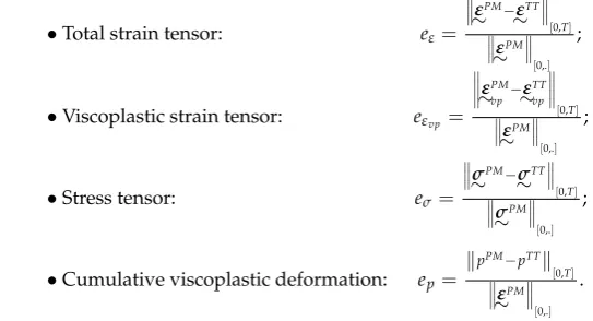
200
•Total strain tensor: eε=
∼ε PM− ε ∼TT
[0,T]
∼ε
PM
[0,.]
;
•Viscoplastic strain tensor: eεvp= ∼ε
PM vp−∼ε
TT vp
[0,T]
∼ε
PM
[0,.]
;
•Stress tensor: eσ=
∼σ PM− σ ∼TT
[0,T]
∼σ
PM
[0,.]
;
•Cumulative viscoplastic deformation: ep=
kpPM−pTTk
[0,T]
∼ε
PM
[0,.]
.
201
Depending on the parameter values, the viscoplastic part of the behavior may or may not be
202
negligible as measured by the magnitudes ofkpkand ∼εvp
relative to ∼ε
. Hence, in the proposed
203
application, the focus is on comparing the norm of the approximation error for∼ε,∼εvp and pwith
204
respect to the norm of∼ε.
205
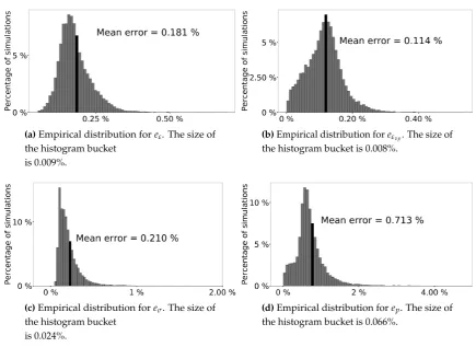
The histograms featured on Figures4a,4b,4cand4dpresent, for each mechanical variables, the
206
empirical distribution of the relative error for all simulation results. The surrogate model given by the
207
tensor-train decompositions features a level of error that is sufficiently low to carry out parametric
208
studies such as calibration of constitutive laws where errors lower than 2% are typically tolerable.
(a)Empirical distribution foreε. The size of the histogram bucket
is 0.009%.
(b)Empirical distribution foreεvp. The size of the histogram bucket is 0.008%.
(c)Empirical distribution foreσ. The size of the histogram bucket
is 0.024%.
(d)Empirical distribution forep. The size of
the histogram bucket is 0.066%.
Figure 4.Empirical distribution of the errors for every mechanical variables.
3.4. Convergence with respect to the truncation tolerance
210
A first surrogate model is constructed from the physical model with the prescribed truncation tolerancee=10−3. Then, this first surrogate model is used as an input for Algorithm1. Running the
algorithm several times with different truncation tolerances:
e∈
n
1×10⁻³; 2×10⁻³; 4.6×10⁻³; 1×10⁻²; 2×10⁻²; 4.6×10⁻²; 1×10⁻¹o
generates as many new surrogate models.
211
Figures6a,6b,6cand6dpresent the evolution of the relative error distribution (for the different
212
mechanical variables) with respect to the truncation tolerance based on a random sample of 20 000
213
parameter set values chosen as in Section3.3. Figure5details the graphical notations. The results
214
empirically show for each mechanical output, the relative error decreases together with e. It is
215
consistent with the expected behavior of the algorithm.
216
Q1 Q3
IQR
Q1- 1.5 x IQR Q3+ 1.5 x IQR
Median
Outliers
Figure 5.The left and right sides are the first and third quartiles (respectively Q1and Q3). The line
(a)Empirical distribution foreε (b)Empirical distribution foreεvp
(c)Empirical distribution foreσ (d)Empirical distribution forep
Figure 6.Empirical distribution of the relative approximation error for every mechanical variables.
Plots in Figure7aand7bshow the dependence of the number of stored elements and the number
217
of calls to the physical model one.
218
(a) Dependence of the number of calls to physical model one
(b) Dependence of the number of stored elements one
Figure 7.Dependence of computational cost and memory storage indicators one
3.5. On fly error estimation
219
Based on the physical model, the surrogate model gives an approximation of each output of
220
interest. However, the approximate outputs may be inconsistent with the physics in the sense that
221
they may lead to non-zero residuals when introduced into (the discrete version of) the DAE system
222
describing the physical model.
223
Acoherence estimatoris an indicator that measures how closely the physical equations are verified
224
by the outputs of the surrogate model. It is reasonable to expect the accuracy of the metamodel to be
225
correlated with the coherence estimator.
Using Equation (A1) let:
σ
∼eq,TT=
E 1+ν
ε
∼TTe +
ν
1−2νTr
ε
∼TTe
I
∼
and define the associated coherence estimator as follows:
ησ = ∼σ
TT−σ ∼eq,TT
[0,T]
∼σ
TT
[0,T]
(17)
Figure8displays the relation between the relative error forσ∼and the effectivity of the estimator
227
ησ/eσfor 20 000 simulation results drawn randomly. The error increases with the final cumulative
228
deformation, that is when the material exhibits a more intense viscoplastic behavior.
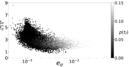
229
Figure 8.Effectivity of the coherence estimatorησ(17) associated withσ. The color scale indicates the final cumulative deformation.
Furthermore, the plot shows a correlation between the coherence estimator and the relative error.
230
In particular, the effectivity tends to be larger than 1 which indicates that the coherence estimator
231
behaves like an upper bound of the relative error. Excluding a few outliers, the coherence estimator
232
does not overestimate the relative error by more than a factor 7.
233
Finally, the effectivity of the coherence estimator empirically converges to 1 (that is, the estimator
234
becomes sharper) as the magnitude of the relative error increases.
235
This coherence estimator is very cheap to compute and only relies on outputs of the surrogate
236
model. The results suggest that the coherence estimator could be used as an online error indicator that
237
increases the reliability of the surrogate model at the current point when exploring in real-time the
238
parameter domain.
239
4. Discussion
240
The present work assesses the performance of tensor-train representations for the approximation
241
of numerical solutions of nonlinear DAE systems. The proposed method enables to incorporate a
242
large number of simulation results ('500 000 scalar values) to produce a metamodel that is accurate
243
over the entire parameter domain. More specifically, numerical results show that the Multiple TT
244
decomposition gives promising results when used as a surrogate model for an elasto-viscoplastic
245
constitutive law. For this particular application, the surrogate model exhibits a satisfying accuracy
246
given the moderate computational effort spent for its construction and the data storage requirements.
247
Moreover, the observed behavior of the proposed empirical coherence estimator indicates that the
248
latter could be exploited to assess the approximation error in real time.
249
The application to more complex material constitutive laws of industrial interest and involving a
250
larger number of parameters [32] corroborate the aforementioned results in terms of compactness and
251
accuracy of the surogate models. Surrogate models have the potential to transform the way of carrying
252
out parametric studies in material science. In particular, [32] demonstrates that the exploitation of
models based on the Multiple TT approach simplifies the process of calibration of constitutive laws.
254
Future work will investigate the combination of the proposed method with “usual” model order
255
reduction techniques such as hyper-reduction [33] in order to take into account the space dimension.
256
Author Contributions:Conceptualization, D.R.; Methodology, C.O., D.R. and J.C.; Software, C.O.; Validation,
257
C.O.; Formal Analysis, C.O. and J.C.; Investigation, C.O.; Resources, J.C.; Data Curation, C.O.; Writing - Original
258
Draft Preparation, C.O.; Writing - Review & Editing, D.R. and J.C.; Visualization, C.O.; Supervision, D.R. and J.C.;
259
Project Administration, J.C.; Funding Acquisition, D.R. and J.C.;
260
Funding:This research was funded by the Association Nationale de la Recherche et de la Technologie (ANRT)
261
[grant number CIFRE 2014/0923].
262
Acknowledgments:The authors gratefully acknowledge fruitful discussions with Safran Helicopter Engines.
263
Conflicts of Interest:The authors declare no conflict of interest. The founding sponsors had no role in the design
264
of the study; in the collection, analyses, or interpretation of data; in the writing of the manuscript, and in the
265
decision to publish the results.
266
Abbreviations
267
The following abbreviations are used in this manuscript:
268 269
DAE Differential Algebraic Equation
DEIM Discrete Empirical Interpolation Method DOAJ Directory of Open Access Journals EIM Empirical Interpolation Method PGD Proper Generalized Decomposition POD Proper Orthogonal Decomposition PSD Pseudo-Skeleton Decomposition SVD Singular Value Decomposition TT Tensor Train
270
Appendix A Elasto-viscoplastic model
271
The application case consists of a nonlinear constitutive law in elasto-viscoplasticity [34,35] linking
272
the following time-dependent mechanical variables:
273
• The strain tensor:∼ε=∼εe+∼εvp[Dimensionless] (sum of an elastic part and a viscoplastic part);
274
• The stress tensor:σ∼[MPa];
275
• An internal hardening variable: X∼[MPa];
276
• The cumulative viscoplastic deformation: p[Dimensionless].
277
where∼ε,∼εe,∼εvp,∼σandX∼are second order tensors inR3×3.
278
The hypotheses of the infinitesimal strain theory are assumed to hold.
279
The model involves eight material coefficients:E,ν,n,K,R0,Q,bandC. The Young and Poisson
280
coefficients are set toE=200 000 MPa andν=0.3. TableA1presents the range of variation of the
281
other material coefficients considered as inputs parameters of the model.
Table A1.Parameter range of variations considered in the model. When applicable, the unit is indicated between brackets.
n K[MPa.s-n] R
0[MPa] Q[MPa] b C[MPa]
Lower bound 2 100 1 1 0.02 150
Upper bound 12 10 000 200 2 000 2 000 150 000
282
Appendix A.0.1 System of equations
283
The elastic behavior is governed by:
σ
∼=
E 1+ν
ε
∼e+
ν
1−2νTr
ε
∼e
I
∼
The viscoplastic behavior is described by the Norton flow rule (A2) formulated with the von
284
Mises criterion (A5). The yield function and the normal to the yield function are given by (A3) and
285
(A4). (A6) gives the definition of the deviatoric stress tensor involved in (A5).
286
d
dt∼εvp=N∼
f K
n +
(A2)
f = J∼σD−X∼
−R (A3)
N∼= 3 2
σ
∼D−X∼
Jσ∼D−X∼
(A4)
J∼σD−X∼
= r
3 2
σ
∼D−X∼
:∼σD−X∼
(A5)
σ
∼D=σ∼−
1 3Tr
σ
∼
I
∼ (A6)
where(.)+denotes the positive part function.
287
The operator:denotes the contracted product defined as:
Z
∼1:∼Z2= 3
∑
i=13
∑
j=1Z1ijZij2 for ∼Z1,∼Z2∈R3×3
The nonlinear isotropic hardening is modeled by (A7) where (A8) gives the viscoplastic
288
cumulative rate.
289
R=R0+Q
1−e−bp (A7)
dp dt =
r 2 3
d dt∼εvp:
d
dt∼εvp (A8)
Finally the linear kinematic hardening is given by:
X∼= 2
3C∼εvp (A9)
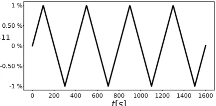
The case of a uniaxial cyclic tensile testing driven by deformation is considered. The loading
290
is applied by imposingε11(t)with the pattern shown in FigureA1andσ12(t) =σ13(t) = σ23(t) =
291
σ22(t) =σ33(t) =0.
292
0 200 400 600 800 1000 1200 1400 1600
t[s]
-1 % -0.50 % 0 % 0.50 % 1 %
11
Figure A1.The applied strain componentε11(t)consists of a triangular pattern of period 400s with a
The initial conditions for the internal variables are:
p(t=0) =0 and X∼(t=0) =∼0
The model is highly nonlinear. First the isotropic hardening law introduces an exponential
293
nonlinearity. The most significant nonlinearity arises from the Norton law (A2) featuring the positive
294
part function. Capturing the resulting threshold effect is particularly challenging for surrogate models.
295
References
296
1. Ghighi, J.; Cormier, J.; Ostoja-Kuczynski, E.; Mendez, J.; Cailletaud, G.; Azzouz, F. A microstructure
297
sensitive approach for the prediction of the creep behaviour and life under complex loading paths.
298
Technische Mechanik2012,32, 205–220.
299
2. Le Graverend, J.B.; Cormier, J.; Gallerneau, F.; Villechaise, P.; Kruch, S.; Mendez, J. A
300
microstructure-sensitive constitutive modeling of the inelastic behavior of single crystal nickel-based
301
superalloys at very high temperature.International Journal of Plasticity2014,59, 55–83.
302
3. Ladevèze, P.; Nouy, A. On a multiscale computational strategy with time and space homogenization
303
for structural mechanics. Computer Methods in Applied Mechanics and Engineering2003,192, 3061 – 3087.
304
Multiscale Computational Mechanics for Materials and Structures.
305
4. Ammar, A.; Mokdad, B.; Chinesta, F.; Keunings, R. A new family of solvers for some classes of
306
multidimensional partial differential equations encountered in kinetic theory modeling of complex fluids.
307
Journal of Non-Newtonian Fluid Mechanics2006,139, 153 – 176.
308
5. Nouy, A. A priori model reduction through Proper Generalized Decomposition for solving time-dependent
309
partial differential equations.Computer Methods in Applied Mechanics and Engineering2010,199, 1603 – 1626.
310
6. Hitchcock, F.L. The Expression of a Tensor or a Polyadic as a Sum of Products.Journal of Mathematics and 311
Physics1927,6, 164–189.
312
7. Khoromskij, B.N. Tensors-structured numerical methods in scientific computing: Survey on recent
313
advances.Chemometrics and Intelligent Laboratory Systems2012,110, 1–19.
314
8. Grasedyck, L.; Kressner, D.; Tobler, C. A literature survey of low-rank tensor approximation techniques.
315
GAMM-Mitteilungen2013,36, 53–78.
316
9. Bigoni, D.; Engsig-Karup, A.P.; Marzouk, Y.M. Spectral Tensor-Train Decomposition. SIAM Journal on 317
Scientific Computing2016,38, A2405–A2439.
318
10. Harshman, R.A. Foundations of the PARAFAC procedure: Models and conditions for an" explanatory"
319
multi-modal factor analysis. UCLA Working Papers in Phonetics1970,16, 1–84.
320
11. Kiers, H.A. Towards a standardized notation and terminology in multiway analysis. Journal of chemometrics 321
2000,14, 105–122.
322
12. Tucker, L.R. The extension of factor analysis to three-dimensional matrices. Contributions to mathematical 323
psychology1964,110119.
324
13. Hackbusch, W.; Kühn, S. A new scheme for the tensor representation. Journal of Fourier analysis and 325
applications2009,15, 706–722.
326
14. Oseledets, I.; Tyrtyshnikov, E. TT-cross approximation for multidimensional arrays. Linear Algebra and its 327
Applications2010,432, 70–88.
328
15. Oseledets, I.V. Tensor-Train Decomposition.SIAM Journal on Scientific Computing2011,33, 2295–2317.
329
16. Savostyanov, D.; Oseledets, I. Fast adaptive interpolation of multi-dimensional arrays in tensor train
330
format. Multidimensional (nD) Systems (nDs), 2011 7th International Workshop on, 2011, pp. 1–8.
331
17. Savostyanov, D.V. Quasioptimality of maximum-volume cross interpolation of tensors. Linear Algebra and 332
its Applications2014,458, 217–244.
333
18. Sirovich, L. Turbulence and the Dynamics of Coherent Structures. Part 1: Coherent Structures. Quarterly of 334
Applied Mathematics1987,45, 561–571.
335
19. Everson, R.; Sirovich, L. Karhunen-Loève procedure for gappy data. Journal of the Optical Society of America 336
A1995,12, 1657–1664.
337
20. Maday, Y.; Nguyen, N.C.; Patera, A.T.; Pau, S.H. A general multipurpose interpolation procedure: the
338
magic points. Communications on Pure and Applied Analysis2009,8, 383–404.
21. Barrault, M.; Maday, Y.; Nguyen, N.C.; Patera, A.T. An empirical interpolation method: application to
340
efficient reduced-basis discretization of partial differential equations. Comptes-Rendus Mathématiques2004,
341
339, 667–672.
342
22. Ryckelynck, D.; Lampoh, K.; Quilicy, S. Hyper-reduced predictions for lifetime assessment of elasto-plastic
343
structures. Meccanica2016,51, 309–317.
344
23. Carlberg, K.; Farhat, C.; Cortial, J.; Amsallem, D. The GNAT method for nonlinear model reduction:
345
Effective implementation and application to computational fluid dynamics and turbulent flows.Journal of 346
Computational Physics2013,242, 623–647.
347
24. Tyrtyshnikov, E.; Goreinov, S.; Zamarashkin, N. Pseudo-Skeleton Approximations. Technical report,
348
Institute of Numerical Mathematics of the Russian Academy of Sci., Leninski Prosp. 32-A Moscow 117334,
349
Russia, 1993.
350
25. Bebendorf, M. Approximation of boundary element matrices. Numerische Mathematik2000,86, 565–589.
351
26. Berry, M.W.; Pulatova, S.A.; Stewart, G. Algorithm 844: Computing sparse reduced-rank approximations
352
to sparse matrices. ACM Transactions on Mathematical Software (TOMS)2005,31, 252–269.
353
27. Stewart, G. Four algorithms for the the efficient computation of truncated pivoted QR approximations to a
354
sparse matrix. Numerische Mathematik1999,83, 313–323.
355
28. Golub, G.H.; Van Loan, C.F.Matrix computations, 4 ed.; The Johns Hopkins University Press, 2013.
356
29. Halton, J.H. On the Efficiency of Certain Quasi-random Sequences of Points in Evaluating
357
Multi-dimensional Integrals. Numer. Math.1960,2, 84–90.
358
30. Drmac, Z.; Gugercin, S. A New Selection Operator for the Discrete Empirical Interpolation
359
Method—Improved A Priori Error Bound and Extensions. SIAM Journal on Scientific Computing2016,
360
38, A631–A648.
361
31. Chaturantabut, S.; Sorensen, D.C. Nonlinear Model Reduction via Discrete Empirical Interpolation.SIAM 362
Journal on Scientific Computing2010,32, 2737–2764.
363
32. Olivier, C. Décompositions tensorielles et factorisations de calculs intensifs appliquées à l’identification de
364
modèles de comportement non linéaire. PhD thesis, PSL Reasearch University, 2017.
365
33. Ryckelynck, D.; Vincent, F.; Cantournet, S. Multidimensional a priori hyper-reduction of mechanical models
366
involving internal variables.Computer Methods in Applied Mechanics and Engineering2012,225–228, 28–43.
367
34. Besson, J.; Cailletaud, G.; Chaboche, J.L.; Forest, S.Non-linear mechanics of materials, 1 ed.; Vol. 167, Springer
368
Netherlands, 2010.
369
35. Lemaitre, J.; Chaboche, J.L.Mechanics of solid materials; Cambridge University Press, 1994.