Can We Trust the Bootstrap in High-dimensions?
The Case of Linear Models
Noureddine El Karoui [email protected], [email protected]
Criteo AI Lab 32 Rue Blanche 75009 Paris, France and
Department of Statistics University of California Berkeley, CA 94270, USA
Elizabeth Purdom [email protected]
Department of Statistics University of California Berkeley, CA 94270, USA
Editor:Guy Lebanon
Abstract
We consider the performance of the bootstrap in high-dimensions for the setting of linear regression, wherep < nbutp/nis not close to zero. We consider ordinary least-squares as well as robust regression methods and adopt a minimalist performance requirement: can the bootstrap give us good confidence intervals for a single coordinate ofβ (whereβ is the true regression vector)?
We show through a mix of numerical and theoretical work that the bootstrap is fraught with problems. Both of the most commonly used methods of bootstrapping for regression— residual bootstrap and pairs bootstrap—give very poor inference on β as the ratio p/n
grows. We find that the residual bootstrap tend to give anti-conservative estimates (inflated Type I error), while the pairs bootstrap gives very conservative estimates (severe loss of power) as the ratiop/n grows. We also show that the jackknife resampling technique for estimating the variance of ˆβ severely overestimates the variance in high dimensions.
We contribute alternative procedures based on our theoretical results that result in dimensionality adaptive and robust bootstrap methods.
Keywords: Bootstrap, high-dimensional inference, random matrices, resampling
1. Introduction
The bootstrap (Efron, 1979) is a ubiquitous tool in applied statistics, allowing for infer-ence when very little is known about the properties of the data-generating distribution. The bootstrap is a powerful tool in applied settings because it does not make the strong assumptions common to classical statistical theory regarding this data-generating distri-bution. Instead, the bootstrap resamples the observed data to create an estimate, ˆF, of the unknown data-generating distribution, F. The distribution ˆF then forms the basis of further inference.
c
Since its introduction, a large amount of research has explored the theoretical properties of the bootstrap, improvements for estimatingF under different scenarios, and how to most effectively estimate different quantities from ˆF (see the pioneering Bickel and Freedman, 1981 for instance and many many more references in the book-length review of Davison and Hinkley, 1997, as well as van der Vaart, 1998 for a short summary of the modern point of view on these questions). Other resampling techniques exist of course, such as subsampling, m-out-of-n bootstrap, and jackknifing, all of which have been studied and much discussed (see Efron, 1982; Hall, 1992; Politis et al., 1999; Bickel et al., 1997; and Efron and Tibshirani, 1993 for a practical introduction).
An important limitation for the bootstrap is the quality of ˆF. The standard bootstrap estimate ofF based on the empirical distribution of the data may be a poor estimate when the data has a non-trivial dependency structure, when the quantity being estimated, such as a quantile, is sensitive to the discreteness of ˆF, or when the functionals of interest are not smooth (see e.g., Bickel and Freedman, 1981 for a classic reference, as well as Beran and Srivastava, 1985 or Eaton and Tyler, 1991 in the context of multivariate statistics).
An area that has received less attention is the performance of the bootstrap in high dimensions and this is the focus of our work. In particular, we consider the setting of standard linear models where data yi are drawn from the linear model
∀i, yi=β0Xi+i ,1≤i≤n , where Xi ∈Rp .
We are interested in the bootstrap or resampling properties of the estimator defined as
b
βρ= argminb∈Rp n X
i=1
ρ(yi−Xi0b), where ρ is a convex function.
We consider the two standard methods for resampling to create a bootstrap distribution in this setting. The first is pairs resampling, where bootstrap samples are drawn from the empirical distribution of the pairs (yi, Xi). The second resampling method is residual resampling, where the bootstrapped data consists ofyi∗=βbρ0Xi+ ˆ∗i, where ˆ∗i is drawn from
the empirical distribution of the estimated residuals, ei. We also consider the jackknife,
a resampling method focused specifically on estimating the variance of functionals of βbρ.
These three methods are extremely flexible for linear models regardless of the method of fittingβ or the error distribution of thei.
The high dimensional setting: p/n→κ∈(0,1) In this work we call a high-dimensional setting one where the number of predictors, p, is of the same order of magnitude as the number of observations, n, formalized mathematically by assuming that p/n→ κ∈(0,1). Several reasons motivate our theoretical study in this regime. The asymptotic behavior of the estimate βbρ is known to depend heavily on whether one makes the classical theoretical
high-dimensional assumption can work surprisingly well in very low-dimension (see John-stone, 2001). Furthermore, in these high-dimensional settings, where much is still unknown theoretically, the bootstrap is a natural and compelling alternative to asymptotic analysis. Another motivation for our investigation is that of very large scale applications (Chapelle et al., 2014; Criteo, 2017; Langford et al., 2007), where one might resort to subsampling methods or recent variants like the bag-of-little-bootstraps (Kleiner et al., 2014) for un-certainty assessment. Subsampling is also very commonly used in this setting for simple computational speed-up. In such cases, even if one had started with a data set where
p n, after subsampling one often ends up with p comparable to n on the subsamples where bootstrap-like computations are performed. It is therefore important to know if the bootstrap and other resampling plans perform well when pis comparable to n.
Defining success: accurate inference on β1 The common theoretical definition of whether the bootstrap “works” is that the bootstrap distribution of the entire bootstrap estimate
b
βρ∗ converges conditionally almost surely to the sampling distribution of the estimatorβbρ
(see e.g., van der Vaart, 1998). The work of Bickel and Freedman (1983) on the residual bootstrap for least squares regression, which we discuss in the background section 1.2, shows that this theoretical requirement is not fulfilled even for the simple problem of least squares regression.
In this paper, we choose to focus only on accurate inference for the projection of our parameter on a pre-specified directionυ. More specifically, we concentrate only on whether the bootstrap gives accurate confidence intervals forυ0β. We think that this is the absolute minimal requirement we can ask of a bootstrap inferential method, as well as one that is meaningful from the standpoint of applied statistics. This is of course a much less stringent requirement than performing well on complicated functionals of the whole parameter vector, which is the implicit demand of standard definitions of bootstrap success. For this reason, we focus throughout the exposition on inference forβ1 (the first element ofβ) as an example of a pre-defined direction of interest (where β1 corresponds to choosing υ = e1, the first canonical basis vector).
We note that considering the asymptotic behavior ofυ0βasp/n→κ∈(0,1) implies that
υ =υ(p) changes with p. By “pre-defined” we will mean simply a deterministic sequence of directions υ(p). We will continue to suppress the dependence on p in writing υ in what follows for the sake of clarity.
1.1 Organization and Main Results of the Paper
In Section 2 we demonstrate that in high dimensions residual-bootstrap resampling results in extremely poor inference on the coordinates ofβρ with error rates much higher than the
reported Type I error. We show that the error in inference based on residual bootstrap resampling is due to the fact that the distribution of the residuals ei are a poor estimate
of the distribution ofi; we further illustrate that common methods of standardizing theei
do not solve the problem for general ρ. We propose two new dimension-adaptive methods of residual resampling that appear promising for use in bootstrapping linear models. We also provide some theoretical results for the behavior of this method asp/n→1.
case discussed in Section 2, the confidence intervals obtained from the pairs-bootstrap are instead conservative to the point of being non-informative. This results in a dramatic loss of power. We prove in the case ofL2 loss, i.e.,ρ(x) =x2, that the variance of the bootstrapped
v0βb∗ is greater than that of v0βb, leading to the overly conservative performance we see in
simulations. We demonstrate that a different resampling scheme we propose can provide accurate confidence intervals in moderately high dimensions.
In Section 4, we discuss another resampling scheme, the jackknife. We focus on the jackknife estimate of variance and show that it has similarly poor behavior in high dimen-sions. In the case of L2 loss with Gaussian design matrices, we further prove that the jackknife estimator over estimates the variance of our estimator by a factor of 1/(1−p/n); we also provide corrections for other losses that improve the jackknife estimate of variance in moderately high dimensions.
We rely on simulation results to demonstrate the practical impact of the failure of the bootstrap. The settings for our simulations and corresponding theoretical analyses are ide-alized, without many of the common settings of heteroskedasticity, dependency, outliers and so forth that are known to be a problem for bootstrapping. This is intentional, since even these idealized settings are sufficient to demonstrate that the standard bootstrap methods have poor performance. For brevity, we give only brief descriptions of the simulations in what follows; detailed descriptions can be found in AppendixD.1.
Similarly, we focus on the basic implementations of the bootstrap for linear models. While there are many proposed alternatives (often for specific loss functions or types of data), the standard methods we study are most commonly used and recommended in prac-tice. Furthermore, to our knowledge none of the alternative bootstrap methods we have seen specifically address the underlying theoretical problems that appear in high dimensions without making low-dimensional assumptions about either the design matrix or the sparsity ofβ, and therefore are likely to suffer from the same fate as standard methods. We note that in truly large scale applications, sparsity assumptions are not always made by practitioners (Chapelle et al., 2014; Langford et al., 2007; Criteo, 2017) and it is hence natural to study the performance of estimators outside of sparse settings. We have also experimented with more complicated ways to build confidence intervals (e.g., bias correction methods), but have found their performance to be erratic in high-dimension and offer no improvement.
We first give some background regarding the bootstrap and estimation of linear models in high dimensions before presenting our new results.
1.2 Background: Inference Using the Bootstrap
We consider the settingyi =β0Xi+i, whereE(i) = 0 and var (i) =σ2. The vectorβ is
estimated as minimizing the average loss,
b
βρ= argminb∈Rp n X
i=1
ρ(yi−Xi0b), (1)
Bootstrap methods are used in order to estimate the distribution of the estimate βbρ
under the true data-generating distribution, F. The bootstrap estimates this distribution with the distribution obtained when the data is drawn from an estimate ˆF of F. Following standard convention, we designate this bootstrapped estimator βbρ∗ to note that this is an
estimate of β using loss function ρ when the data-generating distribution is known to be exactly equal to ˆF. Since ˆF is completely specified, we can in principle exactly calculate the distribution of βbρ∗ and use it as an approximation of the distribution ofβbρunderF. In
practice, we simulate B independent draws of size n from the distribution ˆF and perform inference based on the empirical distribution ofβbρ∗b,b= 1, . . . , B.
In bootstrap inference for the linear model, there are two common methods for re-sampling, which results in different estimates ˆF. In the first method, called the residual bootstrap, ˆF is an estimate of the conditional distribution of yi given β and Xi. In this
case, the corresponding resampling method consists of resampling ∗i from an estimate of the distribution of and forming data yi∗ =Xi0βbρ+∗i, from which βb∗ρ is computed. This
method of bootstrapping assumes that the linear model is correct for the mean of y (i.e., that E(yi) = Xi0β); it also assumes fixed Xi design vectors because the sampling is
con-ditional on the Xi. In the second method, called pairs bootstrap, ˆF is an estimate of the
joint distribution of the vector (yi, Xi) ∈ Rp+1 given by the empirical joint distribution
of {(yi, Xi)}ni=1; the corresponding resampling method resamples the pairs (yi, Xi). This
method makes no assumption about the mean structure ofyand, by resampling theXi, also
does not condition on the values ofXi. For this reason, pairs resampling is often considered
to be more generally applicable than residuals resampling (see e.g., Davison and Hinkley, 1997).
1.3 Background: High-dimensional Inference of Linear Models
Recent research shows thatβbρhas very different asymptotic properties whenp/nhas a limit κ that is bounded away from zero than it does in the classical setting where p/n→ 0 (see e.g., Huber, 1973; Huber and Ronchetti, 2009; Portnoy, 1984, 1985, 1986, 1987; Mammen, 1989 forκ= 0; El Karoui et al., 2013 forκ∈(0,1)). A simple example is that the vectorβbρ
is no longer consistent in Euclidean norm when κ > 0. We should be clear, however, that projections on fixed non-random directions such as we consider, i.e.,υ0βbρ, are
√
nconsistent for υ0β, even when κ > 0. In particular, the coordinates of βbρ are
√
n−consistent for the coordinates of β (El Karoui et al., 2013, Lemma 1). Hence, in practice the estimatorβbρ is
still a reasonable quantity to consider.
Bootstrap in high-dimensional linear models Very interesting work exists already in the literature about bootstrapping regression estimators when p is allowed to grow with n
(Shorack, 1982; Wu, 1986; Mammen, 1989, 1992, 1993; Parzen et al., 1994; Koenker, 2005, Section 3.9). With a few exceptions, this work has been in the classical, low-dimensional setting where either p is held fixed or p grows slowly relative to n (i.e., κ = 0 in our notation). For instance, in Mammen (1993), it is shown that under mild technical conditions and assuming that p1+δ/n→ 0, δ >0, the pairs bootstrap distribution of linear contrasts
v0(βbρ∗−βbρ) is in fact very close to the sampling distribution ofv0(βbρ−β) with high-probability,
also allow for increasing dimensions, for example in the case of linear contrasts in robust regression, by making assumptions on the diagonal entries of the hat matrix. In our context, these assumptions would be satisfied only if p/n → 0. Hence those interesting results do not apply to the present study. We also note that Hall (1992, p. 167) contains cautionary notes about using the bootstrap in high-dimension.
While there has not been much theoretical work on the bootstrap in the setting where
p/n → κ ∈ (0,1), one early work of Bickel and Freedman (1983) considered bootstrap-ping scaled residuals for least-squares regression when κ > 0. They show that when
p/n → κ ∈ (0,1), there exists a data-dependent direction c, such that c0βbLS∗ does not
have the correct asymptotic distribution (Bickel and Freedman, 1983, Theorem 3.1, p.39), i.e., its distribution is not conditionally in probability close to the sampling distribution of
c0βbLS. Furthermore, they show that when the errors in the model are Gaussian, under the
assumption that the diagonal entries of the hat matrix are not all close to a constant, the empirical distribution of the residuals is a scaled-mixture of Gaussian, which is not close to the original error distribution.
As we previously explained, in this work we instead only consider inference forpredefined
contrastsυ0β. The important and interesting problems pointed out in Bickel and Freedman (1983) disappear if we focus on fixed, non-data-dependent projection directions. Hence, our work complements the work of Bickel and Freedman (1983) and is not redundant with it.
There has been some recent interest in residual bootstrap methods for penalized likeli-hood methods in high-dimensions (often proposed for the case when p >> n), for example lasso estimates (Chatterjee and Lahiri, 2010, 2011), adaptive lasso estimates (Chatterjee and Lahiri, 2013), de-biased lasso estimates (Belloni et al., 2015; Dezeure et al., 2017), and ridge regression (Lopes, 2014). These bootstrap results make the assumption of sparsity of some form, generally in terms of the number of non-zero components of β, but in the case of Lopes (2014) by the assumption that the design matrix X is nearly low-rank. As explained previously, our work is focused on a very different line of inquiry: the case of a comparatively diffuse signal in β, where there is no reduction of the high-dimensional problem to a low-dimensional approximation.
The role of the distribution of X An important consideration in interpreting theoretical work on linear models in high dimensions is the role of the design matrix X. In classical asymptotic theory, the results can be stated conditionally on X so that the assumptions can be stated in terms of conditions that can be evaluated on any observed design matrix
X. In the high dimensional setting, the available theoretical tools do not yet allow for an asymptotic analysis conditional on X; instead the results make assumptions about the distribution of the entries of X. Theoretical work in the nascent literature for the high dimensional setting usually allows for a fairly general class of distributions for the individual elements of Xi and can handle covariance between the predictor variables. However, the Xi’s are generally considered i.i.d., which limits the ability of any Xi to be too influential
1.4 Notations and Default Conventions
When referring to the Huber loss in a numerical context, we refer (unless otherwise noted) to the default implementation in therlmpackage in R, where the transition from quadratic to linear behavior is at k= 1.345. We callX the design matrix and{Xi}ni=1 its rows. We haveXi ∈Rp. βdenotes the true regression vector, i.e., the population parameter. βbρrefers
to the estimate of β using loss ρ; from this point on, however, we will often drop theρ and refer to simply βb. The i-th residual is denoted as ei, i.e., ei = yi−Xi0βb. Throughout the
paper, we assume that the linear model holds, i.e.,yi=Xi0β+i for some fixedβ ∈Rp and
thati’s are i.i.d. with mean 0 and var (i) =σ2. We callGthe distribution of. When we
need to stress the impact of the error distribution on the distribution of βbρ, we will write
b
βρ(G) or βbρ() to denote our estimate of β obtained assuming thati’s are i.i.d. G.
We denote generically by κ = limn→∞p/n. We restrict ourselves to κ ∈ (0,1). The standard notation βb(i) refers to the leave-one-out estimate of βbwhere the i-th pair (yi, Xi)
is excluded from the regression, and ˜ei(i) , yi−Xi0βb(i) is the i-th predicted error (based
on the leave-one-out estimate of βb). We also use the notation ˜ej(i),yj−Xj0βb(i). The hat
matrix is of course H =X(X0X)−1X0. oP denotes a “little-oh” in probability, a standard
notation (see van der Vaart, 1998). When we say that we work with a Gaussian design
with covariance Σ, we mean that Xi iid
v N(0,Σ). Throughout the paper, the loss function
ρ is assumed to be convex, R 7→ R+. We use the standard notation ψ = ρ0. We finally
assume thatρ is such that there is a unique solution to the robust regression problem—an assumption that applies to all classical losses in the context of our paper.
2. Residual Bootstrap
We first focus on the method of bootstrap resampling where ˆF is the conditional distribution
y|β, X.b In this case the distribution of βb∗ under ˆF is formed by independent resampling
of ∗i from an estimate ˆG of the distribution G that generated i. Then new data yi∗ are
formed asyi∗ =Xi0βb+∗i and the model is fitted to this new data to get βb∗. Generally the
estimate of the error distribution, ˆG, is taken to be empirical distribution of the observed residuals, so that the ∗i are found by sampling with replacement from the ei.
Yet, even a cursory evaluation ofeiin the simple case of least-squares regression (ρ(x) = x2) reveals that the empirical distribution of the e
i may be a poor approximation to the
error distribution ofi. In particular, it is well known thateihas variance equal toσ2(1−hi)
wherehi is the ith diagonal element of the hat matrix. This problem becomes particularly
pronounced in high dimensions. For instance, ifXi iid
vN(0,Σ),hi =p/n+ oP(1) so thatei
has variance approximatelyσ2
(1−p/n), i.e., generally much smaller than the true variance
offor limp/n >0. This fact is also true when assuming more general distributions for the design matrix X (see e.g.,Wachter, 1978; Haff, 1979; Silverstein, 1995; Pajor and Pastur, 2009; El Karoui and Koesters, 2011, where the main results of some of these papers require minor adjustments to get the approximation of hi we just mentioned).
● ●
● ●
0.00
0.05
0.10
0.15
0.20
Ratio (κ)
95% CI Error Rate
0.01 0.30 0.50
(a)L1 loss
● ●
● ●
0.00
0.05
0.10
0.15
0.20
Ratio (κ)
95% CI Error Rate
0.01 0.30 0.50
● ●
● ●
(b) Huber loss
● ●
● ●
0.00
0.05
0.10
0.15
0.20
Ratio (κ)
95% CI Error Rate
0.01 0.30 0.50
●
● ●
●
●
●
Residual Jackknife Pairs Std. Residuals
(c)L2loss
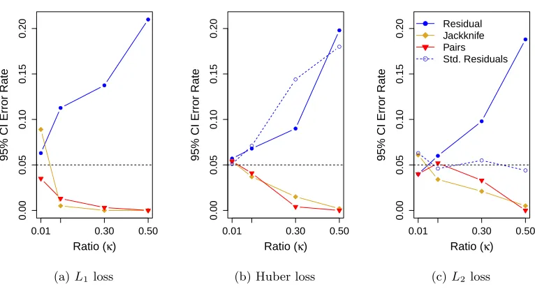
Figure 1: Performance of 95% confidence intervals ofβ1 : Here we show the cover-age error rates for 95% confidence intervals for n= 500 based on applying com-mon resampling-based methods to simulated data: pairs bootstrap (red), residual bootstrap (blue), and jackknife estimates of variance (yellow). These bootstrap methods are applied with three different loss functions shown in the three plots above: (a) L1, (b) Huber, and (c) L2. For L2 and Huber loss, we also show the performance of methods for standardizing the residuals before bootstrapping described in the text (blue, dashed line). If accurate, all of these methods should have an error rate of 0.05 (shown as a horizontal black line). Error rates above 5% correspond to anti-conservative methods. Error rates below 5% correspond to conservative methods. The error rates are based on 1,000 simulations, with
N(0,1) error, and entries of the design matrix i.i.d N(0,1); see the description in Appendix D.1 for more details. The exact values plotted here are given in Table A-1 in Appendix I.
p/n increases the error rate of the confidence intervals in least squares regression increases well beyond the expected 5%: we observe error rates of 10-15% for p/n= 0.3 and approxi-mately 20% forp/n = 0.5. We see similar error rates for other robust-regression methods, such as L1 and Huber loss, and also for different error distributions and distributions of X (Supplementary Figures A-1 and A-2). We explain some of the reasons for these problems in Subsection 2.2 below.
2.1 Bootstrapping from Corrected Residuals
case of least-squares: form corrected residualsri =ei/
√
1−hi and sample the∗i from the
empirical distribution of theri−r¯(see e.g., Davison and Hinkley, 1997).
This correction is known to exactly align the variance of ri with that of i regardless
of the design vectors Xi or the true error distribution, using simply the fact that the hat
matrix is a rankmin(n, p) orthogonal projection matrix. We see that for L2 loss it corrects the error in bootstrap inference in our simulations (Figure 1). This is not so surprising, given that with L2 loss, the error distribution G impacts the inference on β only through
σ2, in the case of homoskedastic errors (see Section 2.4 for much more detail).
However, this adjustment of the residuals is a correction specific to the least-squares problem. Similar corrections for robust estimation procedures using a loss function ρ are given by McKean et al. (1993) with standardized residualsri given by,
ri = ei
√
1−dhi
, where d= 2
P
e0jψ(e0j)
P
ψ(e0j) −
P ψ(e0j)2 (P
ψ(e0j))2, (2)
wherehi is thei-th diagonal entry of the hat matrix,e0j =ej/s,sis a estimate ofσ, and ψ
is the derivative ofρ, assumingψis a bounded and odd function (see Davison and Hinkley, 1997 for a complete description of its implementation for the bootstrap and McKean et al., 1993 for a full description of the regularity conditions).
Unlike the correction for L2 loss mentioned earlier, however, the scaling described in Equation (2) for the residuals is an approximate variance correction, and the approximation depends on assumptions that do not hold true in higher dimensions. The error rate of confidence intervals in our simulations based on this rescaling show no improvement in high dimensions over that of simple bootstrapping of the residuals. This could be explained by the fact that standard perturbation analytic methods used for the analysis of M-estimators in low-dimension, which are at the heart of the correction in Equation (2), fail in high-dimensions.
2.2 Understanding the Behavior of the Residual Bootstrap
This misbehavior of the residual bootstrap can be explained by the fact that in high-dimension, the residuals tend to have a very different distribution from that of the true errors. Their distributions differ not only in simple properties, such as their variances, but in more general aspects, such as their marginal distributions. To make these statements precise, we make use of the previous work of El Karoui et al. (2013) and El Karoui (2013). These papers do not discuss bootstrap or resampling issues, but rather are entirely focused on providing asymptotic theory for the behavior of βbρasp/n→κ∈(0,1); in the course of
doing so, they characterize the asymptotic relationship of ei to i in high-dimensions. We
make use of this relationship to characterize the behavior of the residual bootstrap and to suggest an alternative estimates of ˆGfor bootstrap resampling.
Behavior of residuals in high-dimensional regression We now summarize the asymptotic relationship between ei and i in high-dimensions given in the above cited work (see
Ap-pendixA for a more detailed and technical summary). Letβb(i)be the estimate ofβbased on
For simplicity of exposition,Xi is assumed to have an elliptical distribution, i.e.,Xi=λiΓi,
where Γi ∼N(0,Σ), and λi is a scalar random variable independent of Γi withE λ2i
= 1. For simplicity in restating their results, we will assume Σ = Idp, but equivalent statements
can be made for arbitrary Σ; similar results also apply when Γi = Σ1/2ξi, with ξi having
i.i.d. non-Gaussian entries, satisfying a few technical requirements (see AppendixA). With this assumption on Xi, for any sufficiently smooth loss function ρ and any size
dimension where p/n → κ < 1, the relationship between the i-th residual ei and the true
errori can be summarized as,
˜
ei(i)=i+|λi|kβbρ(i)−βk2Zi+ oP(un) (3) ei+ciλ2iψ(ei) = ˜ei(i)+ oP(un) (4)
where Zi is a random variable distributed N(0,1) and independent of i. The variable un
refers to a sequence of numbers tending to 0. The quantities ci, λi and kβbρ(i)−βk2 are
all of order 1, i.e., they are not close to 0 in general in the high-dimensional setting. The scalar ci is given as n1trace Si−1
,whereSi = 1nPj6=iψ0(˜ej(i))XjXj0. Forp, n large theci’s
are approximately equal andkβbρ(i)−βk2 ' kβbρ−βk2 'E
kβbρ−βk2
; furthermoreciλ2i
can be approximated by Xi0Si−1Xi/n. Note that when ρ is either non-differentiable at all
points (L1) or not twice differentiable (Huber), arguments can be made that make these expressions valid, using for instance the notion of sub-differential forψ(Hiriart-Urruty and Lemar´echal, 2001).
Interpretation of Equations (3) and (4) Equation (3) means that the marginal distribution of the leave-i-th-out predicted error, ˜ei(i), is asymptotically a convolution of the true error,
i, and an independent scale mixture of Normals. Furthermore, Equation (4) means that
thei-th residual ei can be understood as a non-linear transformation of ˜ei(i). As we discuss below, these relationships are qualitatively very different from the classical casep/n→0.
2.2.1 Consequence for the Residual Bootstrap
We apply these results to the question of the residual bootstrap to give an understanding of why bootstrap resampling of the residuals can perform so badly in high-dimension. The distribution of theei is far removed from that of the i, and hence bootstrapping from the
residuals effectively amounts to sampling errors from a distribution that is very different from the original error distribution, .
The impact of these discrepancies for bootstrapping is not equivalent for all dimensions, error distributions, or loss functions. It depends on the constantciand the risk,kβbρ(i)−βk2,
both of which are highly dependent on the dimensions of the problem, the distribution of the errors and the choice of loss function. We now discuss some of these issues.
Least Squares regression In the case of least squares regression, the relationships given in Equation (3) are exact, i.e., un = 0. Further, ψ(x) = x, and ci = hi/(1−hi), giving the
well known linear relationshipei = (1−hi)˜ei(i) (see, e.g., the standard reference Weisberg, 2014). This linear relationship is exact regardless of dimension, though the dimensionality aspects are captured by hi. This expression can be used to show that asymptotically
E Pn i=1e2i
from the residuals results in a distribution that underestimates the variance of the errors by a factor 1−p/n. The corresponding bootstrap confidence intervals are then naturally too small, and hence the error rate increases far from the nominal 5% - as we observed in Figure 1c.
More general robust regression The situation is much more complicated for general robust regression estimators. One clear implication of Equations (3) and (4) is that simply rescaling the residuals ei should not in general result in an estimated error distribution ˆG that will
have similar properties to those ofG. The relationship between the residuals and the errors is very non-linear in high-dimensions. This is why in what follows we will propose to work with leave-one-out predicted errors ˜ei(i) instead of the residualsei.
The classical case of p/n →0: In this setting, ci → 0 and therefore Equation (3) shows
that the residuals ei are approximately equal in distribution to the predicted errors, ˜ei(i). Similarly, βbρ is L2 consistent when p/n → 0, so kβbρ(i)−βk22 → 0 and Equation (4) gives
˜
ei(i) 'i. Hence, the residuals should be fairly close to the true errors in the model when p/nis small. This dimensionality assumption is key to many theoretical analyses of robust regression, and underlies the derivation of corrected residuals ri of McKean et al. (1993)
given in Equation (2) above for losses other thanL2. 2.3 Alternative Residual Bootstrap Procedures
We propose two methods for improving the performance of confidence intervals obtained through the residual bootstrap. Both do so by providing alternative estimates of ˆG from which bootstrap errors ∗i can be drawn. They estimate a ˆG appropriate for the setting of high-dimensional data by accounting for relationship of the distribution of and ˜ei(i).
Method 1: Deconvolution The relationship in Equation (3) says that the distribution of ˜
ei(i) is a convolution of the correct Gdistribution and a normal distribution. This suggests applying techniques for deconvolving a signal from Gaussian noise. Specifically, we propose the following bootstrap procedure: 1) calculate the predicted errors, ˜ei(i); 2)estimate the variance of the normal (i.e.,|λi|kβbρ(i)−βk22);3)deconvolve in ˜ei(i)the error termi from the
normal term;4)Use the resulting estimate ˆG to draw errors∗i for residual bootstrapping. Deconvolution problems are known to be very difficult (see Fan, 1991, Theorem 1 p. 1260, that gives 1/log(n)α rates of convergence when convolving with a Gaussian distribu-tion). The resulting deconvolved errors are likely to be quite noisy estimates ofi. However,
it is possible that while individual estimates are poor, the distribution of the deconvolved errors is estimated well-enough to form a reasonable ˆGfor the bootstrap procedure.
We used the deconvolution algorithm in thedeconpackage in R (Wang and Wang, 2011) to estimate the distribution of i. The deconvolution algorithm requires knowledge of the
variance of the Gaussian that is convolved with the i, i.e., estimation of |λi|kβbρ(i)−βk2
term. In what follows, we assume a Gaussian design, i.e., λi = 1, so that we need to
estimate only the termkβbρ(i)−βk22.An estimation strategy for the more general setting of |λi| 6= 1 is presented in AppendixB.5. We use the fact that kβbρ(i)−βk22 ' kβbρ−βk22 for
all iand estimate kβbρ(i)−βk2 asvard(˜ei(i))−σˆ2,where dvar(˜ei(i)) is the empirical variance
that the deconvolution strategy we employ makes assumptions of homoskedastic errorsi’s,
which is true in our simulations but may not be true in practice. See AppendixB for details regarding the implementation of Method 1.
Method 2: Bootstrapping from standardized e˜i(i) A simpler alternative is bootstrapping from the predicted error terms, ˜ei(i), without deconvolution. Specifically, we propose to bootstrap from a scaled version of ˜ei(i),
˜
ri(i)= q σˆ d var(˜ei(i))
˜
ei(i),
where dvar(˜ei(i)) is the standard estimate of the variance of ˜ei(i) and ˆσ is an estimate of σ. This scaling aligns the first two moments of ˜ei(i) with those of i. On the face of it,
resampling from ˜ri(i)seems problematic, since Equation (3) demonstrates that ˜ei(i) does not have the same distribution asi, even if the first two moments are the same. However, as we
demonstrate in simulations, this distributional mismatch appears to have limited practical effect on our bootstrap confidence intervals.
Estimation ofσ2Both methods described above require an estimator ofσ that is consistent
regardless of dimension and error distribution. As we have explained earlier, for general ρ
we cannot rely on the observed residualsei nor on ˜ei(i)for estimating σ (see Equations (3)
and (4)). The exception is the standard estimate of σ2 from least-squares regression, i.e.,
ρ(x) =x2,
b
σ,LS2 = 1
n−p X
i e2i,L2.
b σ2
,LS is a consistent estimator of σ2 for any error distribution G, assuming i.i.d. errors
and mild moment requirements. In implementing the two alternative residual-bootstrap methods described above, we use bσ,LS as our estimate of σ, including for bootstrapping
robust regression whereρ(x)6=x2.
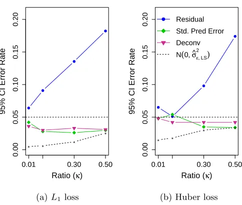
Performance in bootstrap inferenceIn Figure 2 we show the error rate of confidence intervals based on the two residual-bootstrap methods we proposed above. We see that both methods control the Type I error, unlike bootstrapping directly from the residuals, and that both methods are conservative. There is little difference between the two methods with this sample size (n= 500), though withn= 100, we observe the deconvolution performance to be worse in L1 (data not shown).
The deconvolution strategy, however, depends on the distribution of the design matrix, which in these simulations we assumed was Gaussian (so we did not have to estimateλi’s).
For elliptical designs (λi6= 1), the error rate of the deconvolution method described above,
with no adaptation for the design, was similar to that of uncorrected residuals in high dimensions (i.e., > 0.25 for p/n = 0.5). Individual estimates of λi might improve the
● ●
● ●
0.00
0.05
0.10
0.15
0.20
Ratio (κ)
95% CI Error Rate
0.01 0.30 0.50
* * *
*
(a)L1loss
● ●
● ●
0.00
0.05
0.10
0.15
0.20
Ratio (κ)
95% CI Error Rate
0.01 0.30 0.50
* *
* *
● Residual
Std. Pred Error
Deconv
N(0, σ^ε, 2LS)
(b) Huber loss
Figure 2: Bootstrap based on predicted errors: We plotted the error rate of 95% con-fidence intervals for the alternative bootstrap methods described in Section 2.3: bootstrapping from standardized predicted errors (green) and from deconvolution of predicted error (magenta). We demonstrate its improvement over the standard residual bootstrap (blue) for (a)L1 loss and (b) Huber loss. The error distribu-tion is double exponential, but otherwise the simuladistribu-tions parameters are as in Figure 1. The error rates on confidence intervals based on bootstrapping from a
N(0,σb2,LS) (dashed curve) are as a lower bound on the problem. For the precise error rates see Appendix, Table A-3.
Given our previous discussion of the behavior of ˜ei(i), it is somewhat surprising that resampling from the distribution of ˜ri(i) performed well in our simulations. Clearly a few cases exist where ˜ri(i) should work well as an approximation of i. We have already noted
that asp/n→0, the effect of the convolution with the Gaussian disappears sincekβbρ−βk →
0; in this case both ei and ˜ri(i) should be good estimates of i. Similarly, in the case i ∼ N(0, σ2), Equation (3) tells us that ˜ei(i) are also asymptotically marginally normally distributed, so that correcting the variance should result in ˜ri(i)having the same distribution asi, at least whenXi,j are i.i.d.
Surprisingly, for larger p/n we do not see a deterioration of the performance of boot-strapping from ˜ri(i). This is unexpected, since as p/n → 1 the risk kβbρ−βk22 grows to
be much larger than σ2 (a claim we will make more precise in the next section); together with Equation (3), this implies that ˜ri(i) is essentially distributed N(0,bσ
2
,LS) as p/n → 1
regardless of the original distribution of i. This is confirmed in Figure 2 where we
super-impose the results of bootstrap confidence intervals from when we simply estimate ˆGwith
together leads to the conclusion that asp/n →1 we can estimate ˆG simply as N(0,σˆ,LS)
regardless of the actual distribution of .
In the next section we give some theoretical results that seek to understand this phe-nomenon.
2.4 Behavior of the Risk of βbWhen κ→1
In the previous section we saw even if the distribution of the bootstrap errors∗i, given by ˆG, is not close to that of G, we can sometime get accurate bootstrap confidence intervals. For example, in least squares Equation (3) makes clear that even the standardized residuals,ri,
do not have the same marginal distribution as i, yet they still provide accurate bootstrap
confidence intervals in our simulations. We would like to understand for what choice of distributions ˆG will we see the same performance in our bootstrap confidence intervals of
b β1?
When working conditional on X as in residual resampling, the statistical properties of (βb∗ −βb) differ from that of (βb−β) only because the errors are drawn from a different
distribution: ˆGrather than G. Then to understand whether the distribution ofβb1∗ matches
that ofβb1we can ask, what are the distributions of errors,G, that yield the same distribution
for the resultingβb1(G)? In this section, we narrow our focus on understanding not the entire
distribution ofβb1, but only its variance. We do so because under assumptions on the design
matrixX, it is known thatβb1 is asymptotically normally distributed. This is true for both
the classical setting ofκ= 0 and the high-dimensional setting ofκ∈(0,1) (see AppendixA for a review of these results and a more technical discussion). Our previous question is then reduced to understanding which distributions Ggive the same varβb1(G)
.
In the setting of least squares, it is clear that the only property of i iid
v Gthat matters for the variance of βb1,L2 is σ2, since var
b β1,L2
= (X0X)−1(1,1)σ2. For general ρ, if we assume p/n → 0, then var
b β1,ρ
will depend on features of G beyond the first two
moments (specifically throughE ψ2()/[E(ψ0())]2, (Huber, 1973)). If we assume instead
p/n → κ ∈ (0,1), then it has been shown (El Karoui et al., 2013) that var
b β1,ρ(G)
depends on Gonly by the effect ofGon the squared risk of the vector βbρ(G), i.e., through
Ekβbρ(G)−βk22
(for the convenience of the reader we give a review of these results, which are a bit scattered in the literature, in AppendixA).
For this reason, in the setting of p/n→κ∈(0,1), we need to characterize the risk ofβbρ
to understand when different distributions ofresult in the same variance of βb1,ρ. In what
follows, we denote byr2ρ(κ;G) the asymptotic squared risk ofβbρ(G) as pand ntend to∞, rρ2(κ;G) = lim
n,p→∞,np→κE
||βbρ(G)−β||2 .
The dependence ofr2ρ(κ;G) onis characterized, under appropriate technical conditions on X,ρand i’s, by a system of two non-linear equations (El Karoui et al., 2013).
Specifi-cally, if we define ˆz=+rρ(κ;G)Z, whereZ ∼ N(0,1) is independent of , and has the
finite, and deterministic scalars (c, rρ(κ;G)) satisfy the following system of equations:
E((prox(cρ))0(ˆz)) = 1−κ ,
κr2ρ(κ;G) =E [ˆz−prox(cρ)(ˆz)]2
. (5)
In this system, prox(cρ) refers to Moreau’s proximal mapping of the convex functioncρ(see Moreau, 1965; Hiriart-Urruty and Lemar´echal, 2001).
It is therefore not entirely trivial to characterize those distributions Γ for whichr2ρ(κ;G) =
rρ2(κ; Γ). In the following theorem, however, we show that asκ→1,rρ2(κ;G) converges to a constant that depends only onσ2. This implies that whenκ→1, two different error distri-butions that have the same variances will result in estimatorsβb1,ρ with the same variance.
Before stating our theorem formally, however, we will review the necessary assumptions for the system of equations in (5) to hold. For a precise statement of the assumptions, see El Karoui (2017)
Assumptions for Equation 5: The proof of (5) provided in El Karoui (2013) assumes that the Xi’s have mean 0, cov (Xi) = Idp, and they satisfy sub-Gaussian concentration
assumptions (with constants dependent on n). El Karoui (2013) further assumes that the
i have a unimodal density, are independent from theXij, sup1≤i≤n|i|= OP(polyLog(n)),
and that similiar bounds also hold for a few moments of i (the number of such moments
depends on the loss function ρ). Log-concave densities such as those corresponding to double exponential or Gaussian errors used in the current paper fall within the scope of this theorem. The reader interested in generalizations and truly heavy-tailed situation is referred to El Karoui (2017) and references therein.
The loss function ρ is assumed by El Karoui (2013) (in the unpenalized case) to be non-negative, twice differentiable, strongly convex, non-linear, taking value 0 at 0, and with a derivative that grows at most polynomially at infinity and a second derivative that is locally Lipschitz, with local Lipschitz constant that grow at most polynomially at infinity. It should be noted that distributions with sufficiently many moments, the condition of strong convexity of ρ can be obtained by adding δx2/2 to the initial ρ, with δ “small”, e.g., δ = 10−10, and that modification will change very little or anything to the estimator. Furthermore, the requirement of strong convexity ofρ, though superficially limiting, is likely an artifact of the proof, where the main motivation was log-concave distributions with an eye towards optimality (Bean et al., 2013). In fact, the theoretical predictions of (5) were verified numerically in El Karoui et al. (2011) outside of the assumptions stated above, and the predictions of Equation (5) were found to be very accurate in simulations even for non-smoothed`1 and Huber losses with certain error distributions.
We now state the theorem formally; see AppendixE for the proof of this statement.
Theorem 1 Suppose we are working with robust regression estimators with loss ρ, and p/n→κ. Suppose that r2ρ(κ;G) is characterized by the system of equations in (5). Then,
lim
κ→1 1−κ
σ2
rρ2(κ;G) = 1,
Implications for the Bootstrap For the purposes of the residual-bootstrap, Theorem 1 im-plies that different methods of estimating the residual distribution ˆG will result in similar residual-bootstrap confidence intervals asp/n→1, if ˆGhas the same variance. This agrees with our simulations, where both of our proposed bootstrap strategies set the variance of ˆG
equal to bσ
2
,LS and both had similar performance in our simulations for largep/n.
Further-more, as we noted, for p/n closer to 1, they both had similar performance to a bootstrap procedure that simply sets ˆG = N(0,σb2,LS) (Figure 2) (see also AppendixA.3 for further discussion of residual bootstrap methods which draw from the “wrong” distribution, i.e., forms of wild bootstraps (Wu, 1986)).
We return specifically to the bootstrap based on ˜ri(i), the standardized predicted errors. Equation (3) tells us that the marginal distribution of ˜ei(i)is a convolution of the distribution ofiand a normal, with the variance of the normal governed by the termkβbρ−βk2. Theorem
1 makes rigorous our previous assertion that as p/n → 1,the normal term will dominate and the marginal distribution of ˜ei(i)will approach normality, regardless of the distribution of . However, Theorem 1 also implies that as p/n→1,inference for the coordinates of β
will be increasingly less reliant on features of the error distribution beyond the variance, implying that our standardized predited errors, ˜ri(i), will still result in an estimate ˆG that will give accurate confidence intervals. Conversely, asp/n→0 classical theory tells us that the inference ofβ relies heavily on the distributionGbeyond the first two moments, but in that case the distribution of ˜ri(i)approaches the correct distribution as we explained earlier. So bootstrapping from the marginal distribution of ˜ri(i)also makes sense whenp/nis small. For κ between these two extremes it is difficult to theoretically predict the risk of
b
βρ( ˆG) when the distribution ˆGis given by resampling from the ˜ri(i). We turn to numerical simulations to evaluate this risk. Specifically, for i ∼ G, we simulated data that is a
convolution ofGand a normal with variance equal torρ2(κ;G); we then scale this simulated data to have variance σ2. The scaled data are the∗i and we refer to the distribution of∗i
as the convolution distribution, denoted Gconv. Then, Gconv is the asymptotic version of
the marginal distribution of the standardized predicted errors, ˜ri(i), used in our bootstrap method proposed above.
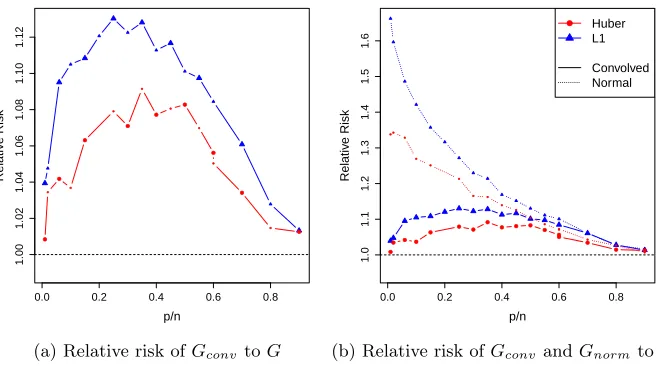
In Figure 3 we plot for both Huber loss and L1 loss the average risk rρ(κ;Gconv) (i.e.,
errors given byGconv) relative to the average riskrρ(κ;G) (i.e., errors distributed according
to G), where G has a double exponential distribution. We also plot the relative average risk rρ(κ;Gnorm), where Gnorm = N(0, σ2). As predicted by Theorem 1, for κ close to
1, rρ(κ;Gconv)/rρ(κ;G) and rρ(κ;Gnorm)/rρ(κ;G) converge to 1. Conversely, as κ → 0, rρ(κ;Gnorm)/rρ(κ;G) diverges dramatically from 1, whilerρ(κ;Gconv)/rρ(κ;G) approaches
1, as expected. For Huber, the divergence of rρ(κ;Gconv)/rρ(κ;G) from 1 is at most 8%,
but the difference is larger forL1 (12%), probably due to the fact that the convolution with a normal error has a larger effect on the risk forL1.
3. Pairs Bootstrap
As described above, estimating the distribution ˆF from the empirical distribution of (yi, Xi)
(pairs bootstrapping) is generally considered the most general and widely applicable method of bootstrapping, allowing for the linear model to be incorrectly specified (i.e.,E(yi) is not
0.0 0.2 0.4 0.6 0.8 1.00 1.02 1.04 1.06 1.08 1.10 1.12 p/n Relativ e Risk ● ● ● ● ● ● ● ● ● ● ● ● ● ● ● ● ●
(a) Relative risk ofGconv toG
0.0 0.2 0.4 0.6 0.8
1.0 1.1 1.2 1.3 1.4 1.5 1.6 p/n Relativ e Risk ● ● ●● ● ● ● ● ● ● ● ● ● ● ● ● ● ●● ● ● ● ● ● ● ● ● ● ● ● ● ● ● ● ● Huber L1 Convolved Normal
(b) Relative risk ofGconv andGnorm toG
Figure 3: Relative Risk ofβbfor scaled predicted errors vs original errors -
popu-lation version: (a) Plotted with a solid lines are the ratios of the average risk of
b
β(Gconv) to the average risk of βb(G) for Huber andL1 loss. (b) shows the same
plot, but added to the plot (dotted lines) is the relative risk of βb(G) when the
errors are distributed Gnorm = N(0, σ2) . For both figures, the y-axis gives the
relative risk, and the x-axis is the ratio p/n, with n fixed at 500. Blue/triangle plotting symbols indicateL1loss; red/circle plotting symbols indicate Huber loss. The average risk is calculated over 500 simulations, where the design matrix X
has Gaussian entries. The “true” error distribution Gis the standard Laplacian distribution withσ2= 2. Each simulation uses the standard estimate ofσ2 from the generated i’s. rρ(κ;G) was computed using a first run of simulations with
i iidv G. The Huber loss in this plot is Huber1 and not the default Huber1.345 of therlmfunction.
to bootstrapping from the residuals. In the case of random design, it makes also a lot of intuitive sense to use the pairs bootstrap, since resampling the predictors might be interpreted as mimicking the data generating process.
However, as in residual bootstrap, it is clear that the pairs bootstrap will have problems, at least in quite high dimensions. In fact, when resampling the Xi’s from ˆF, the number
of times a certain vector Xi0 is picked has asymptotically Poisson(1) distribution. So the
expected number of different vectors appearing in the bootstrapped design matrix X∗ is
dramatically as the dimension increases, becoming increasingly conservative (Figure 1). In pairs bootstrapping, the error rates of 95%-confidence-intervals drop far below the nominal 5%, and are essentially zero for the ratio ofp/n= 0.5. Like residual bootstrap, this overall trend is seen for all the settings we simulated under (Supplemental Figures A-1, A-2). For
L1 loss, even ratios as small as 0.1 yield incredibly conservative bootstrap confidence inter-vals for βb1, with the error rate dropping to less than 0.01. For Huber and L2 losses, the
severe loss of power in our simulations starts for ratios of 0.3.
A minimal requirement for the distribution of the bootstrapped data to give reasonable inferences is that the variance of the bootstrap estimator βb∗1 needs to be a good estimate
of the variance of βb1. This is not the case in high-dimensions. In Figure 5 we plot the
ratio of the variance of βb1∗ to the variance of βb1 evaluated over simulations. We see that
forp/n= 0.3 and design matrices X with i.i.d. N(0,1) entries, the average variance of βb1∗
roughly overestimates the true variance ofβb1 by a factor 1.3 in the case of least-squares; for
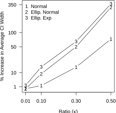
Huber and L1 the bootstrap estimate of variance is roughly twice as large as it should be. In the case of least-squares, we can further quantify this loss in power by comparing the size of the bootstrap confidence intervals to the size of the correct confidence interval based on theoretical results (Figure 4). We see that even for ratios κ as small as 0.1, the confidence intervals for some design matrices X were 15% larger for pairs bootstrap than the correct size (e.g., the case of elliptical distributions whereλi is exponential). For much
higher dimensions of κ= 0.5, the simple case of i.i.d. normal entries for the design matrix gives intervals that are 80% larger than needed; for the elliptical distributions we simulated, the width of the bootstrap confidence interval was as much as 3.5 times larger than that of the correct confidence interval. Furthermore, as we can see in Figure 1, least-squares regression represents the best case scenario; L1 and Huber will have even worse loss of power and at smaller values ofκ.
3.1 Theoretical Analysis for Least-Squares
In the setting of least-squares, we can for some distributions of the design matrix X theo-retically determine the asymptotic expectation of the variance ofv0βb∗ and show that it is a
severe over-estimate of the true variance ofv0βb.
We first setup some notation for the theorem that follows. Define βbw as the result of
regressing y on X with random weightwi for each observation (yi, Xi). In other words,
b
βw= argminu∈Rp n X
i=1
wi(yi−Xi0u)2 .
We assume that the weights are independent of{yi, Xi}ni=1 and defineβb∗w to be the random
variable with distribution equal to that ofβbw conditional on the data{yi, Xi}ni=1, i.e.,βb∗w
L =
b
βw|{yi, Xi}ni=1. For the standard pairs bootstrap, the distribution of βb∗ from resampling
from the pairs (yi, Xi) is equivalent to the distribution of βbw∗, where w is drawn from a
1 1
1
1
Ratio (κ)
% Increase in A
v
er
age CI Width
2 2
2
2
3 3
3
3
0.01 0.10 0.30 0.50
1 10 50 100
350 1
2 3
Normal Ellip. Normal Ellip. Exp
We have the following result for the expected value of the bootstrap variance of any contrast v0βbw∗ where v is deterministic, assuming independent weights with a Gaussian
design matrixX and some mild conditions on the distribution of thew’s.
Theorem 2 Let the weights(wi)ni=1 be i.i.d. and without loss of generality thatE(wi) = 1; we suppose that the wi’s have 8 moments and for all i,wi > η >0. Suppose Xi’s are i.i.d.
N(0,Σ), Σis positive definite and the vector v is deterministic with kvk2= 1.
Suppose βb is obtained by solving a least-squares problem and yi =Xi0β +i, i’s being i.i.d. mean 0, with var (i) =σ2.
If limp/n=κ <1 then the expected variance of the bootstrap estimator, asymptotically as n→ ∞, is given by
p
E
var
v0βbw∗
v0Σ−1v =p E
var
v0βbw|{yi, Xi}ni=1
v0Σ−1v →σ
2
κ
1−κ−f(κ) − 1 1−κ
,
where f(κ) =E
1 (1+cwi)2
and c is the unique solution of E
1 1+cwi
= 1−κ.
We note thatE
1 (1+cwi)2
≥hE
1 1+cwi
i2
= (1−κ)2 - where the first inequality comes from Jensen’s inequality, and therefore the expression we give for the asymptotic limit of the expected bootstrap variance is non-negative. For a proof of this theorem and a consistent estimator of this limit, see AppendixF.
In light of previous work on model robustness issues in high-dimensional statistics (see e.g., (Diaconis and Freedman, 1984; Hall et al., 2005; El Karoui, 2009, 2010)), it is natural to ask whether the central results of Theorem 2 still apply when Xi is not Gaussian but
has an elliptical distribution. The formula in Theorem 2 does not apply directly to this latter case. However, the proof given in AppendixF extends to that setting, and we refer the interested reader to the AppendixF.1 where we give the necessary details of how to change the formulas and proof to encompass the elliptical case (we do not provide them in rigorous mathematical detail in this work as they are substantially more cumbersome than those in Theorem 2 and do not give enough additional insights to justify inclusion). On the other hand, a number of the quantities appearing in the proof of Theorem 2 will converge to the same limit as that given in Theorem 2 when i.i.d. Gaussian predictors are replaced by i.i.d. predictors with mean 0 and variance 1 and sufficiently many moments (an example being bounded random variables). Thus the results we present here should be fairly robust to changing i.i.d. normality assumptions for the entries of the design matrixX, but again the technical work necessary for making this rigorous is beyond the scope of this paper.
Implications for Pairs Bootstrap In the standard pairs bootstrap, the weights are chosen according to a Multinomial(n,1/n) distribution. This violates two conditions in the previ-ous theorem: independence of wi’s and the condition wi>0. In AppendixF.2, we give the
When Xi iid
v N(0,Σ), it is well known in the least-squares case that the quantity
p var
v0βb
/v0Σ−1v converges asymptotically to κ/(1−κ)σ2 (this can be shown through simple Wishart computations Haff, 1979; Mardia et al., 1979). If the variance ofv0βbw∗
con-verged to the variance of v0βb, we should be able to equate this latter quantity to the limit
given in Theorem 2, i.e.,
κ
1−κ−f(κ) − 1 1−κ
= κ 1−κ ,
and hence should have
f(κ) =E
1 (1 +cwi)2
= 1−κ 1 +κ .
However, this relationship does not hold for most weight distributions, and in partic-ular does not hold for weights following a Poisson(1) distribution (which asymptotically corresponds to the standard pairs bootstrap, as explained above). Thus the pairs bootstrap does not correctly estimate the variance of v0βb. In Figure 5a we calculate the theoretical
predictions of E
var
b βw∗
given by Theorem 2 (using Poisson(1) weights and Σ = Idp),
and we compare them to the asymptotic variance ofβb1 given byκ/(1−κ)σ2/p. We see that
Theorem 2 predicts that the pairs bootstrap overestimates the variance of the estimator by a factor that ranges from 1.2 to 3 as κ varies between 0.3 and 0.5. These theoretical predictions correspond to the level of overestimation of the variance seen in our bootstrap simulations (Figure 5b).
3.2 Alternative Weight Distributions for Resampling
The formula given in Theorem 2 suggests that resampling from a distribution ˆF defined using weights other than i.i.d. Poisson(1) (or, equivalently for our asymptotics,
Multinominal(n,1/n)) should give us better bootstrap estimators than using the standard pairs bootstrap. In fact, we should require, at least, that the bootstrap expected variance of these estimators match the correct variance varv0βb
=κ/(1−κ)σ2/p(for the Gaussian design, when Σ = Idp). We focus our discussion on the case Σ = Idp; see AppendixC for
the case Σ6= Idp.
We note that if we use wi = 1, ∀i, the bootstrap variance will be 0, since with such
a resampling scheme the resampled data set is always the original data set. On the other hand, we have seen that with wi ∼ Poisson(1), the expected bootstrap variance was too
large compared toκ/(1−κ)σ2/p. Hence, we tried to find alternative weights via calculating a parameter α such that if
wi iid
v1−α+αPoisson(1), (6)
the expected bootstrap variance would match the theoretical value of κ/(1−κ)σ2/p. We numerically solved this problem to find α(κ) (for details of computation see Ap-pendixC). We then used these values and performed bootstrap resampling using the weights defined in Equation (6). We evaluated bootstrap estimate of varβb1
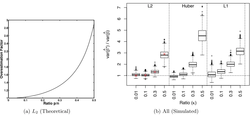
0 0.1 0.2 0.3 0.4 0.5 1 1.2 1.4 1.6 1.8 2 2.2 2.4 2.6 2.8 3 Ratio p/n Overestimation Factor
(a)L2 (Theoretical)
● ● ● ● ● ● ● ● ● ● ● ● ● ● ● ● ● ● ● ● ● ● ● ● ● ● ● ● ● ● ● ● ● ● ● ● ● ● ● ● ● ● ● ● ● ● ● ● ● ● ● ● ● ● ● ● ● ● ● ● ● ● ● ● ● ● ● ● ● ● ● ● ● ● ● ● ● ● ● ● ● ● ● ● ● ● ● ● ● ● ● ● ● ● ● ● ● ● ● ● ● ● ● ● ● ● ● ● ● ● ● ● ● ● ● ● ● ● ● ● ● ● ● ● ● ● ● ● ● ● ● 1 2 3 4 5 6 7
Ratio (κ)
var(
β
^ *) / v
ar(
β
^ )
0.01 0.1 0.3 0.5 0.01 0.1 0.3 0.5 0.01 0.1 0.3 0.5
L2 Huber L1
(b) All (Simulated)
Figure 5: Factor by which standard pairs bootstrap over-estimates the variance: (a) plotted is the ratio of the value of the expected bootstrap variance computed from Theorem 2 using Poisson(1) weights to the asymptotic varianceκ/(1−κ)σ2. (b) boxplots of the ratio of the bootstrap variance of βb1∗ to the variance βb1,
as calculated over 1000 simulations (i.e., var
b β
is estimated across simulated design matricesX, and not conditional onX). The theoretical prediction for the mean of the distribution from Theorem 2 is marked with a ‘X’ forL2 regression. Simulations were performed with normal design matrix X and normal error i
with values ofn= 500. For the median values of each boxplot, see Table A-6 in AppendixI.
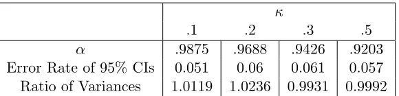
estimating ˆF results in accurate bootstrap estimates of variance and appropriate levels of confidence interval coverage (Table 1).
However, small changes in the choice of α can result in fairly large changes in E
var
v0βbw|X,
. For instance, forκ = 0.5, using the value of α = 0.95 which is close to the correct value ofα(0.5) = 0.92 results in an expected bootstrap variance roughly 30% larger than it should be.
κ
.1 .2 .3 .5
α .9875 .9688 .9426 .9203 Error Rate of 95% CIs 0.051 0.06 0.061 0.057 Ratio of Variances 1.0119 1.0236 0.9931 0.9992
Table 1: Summary of weight-adjusted bootstrap simulations forL2: Given are the results of performing bootstrap resampling for n= 500 according to the estimate of ˆF given by the weights in Equation (6). “Error Rate of 95% CIs” denotes the percent of bootstrap confidence intervals that did not contain the correct value of the parameter β1. “Ratio of Variances” gives the ratio of the empirical expected bootstrap variance over our simulations divided by the theoretical value
σ2κ/(1−κ). Results are based on 1000 simulations, with a Gaussian random design and errors distributed as double exponential.
4. The Jackknife
In the context we are investigating, where we know that the distribution of βb1 is
asymp-totically normal, it is natural to ask whether we could simply use the jackknife to estimate the variance of βb1. The jackknife relies on leave-one-out procedures to estimate var
b β1
.
More specifically, for a fixed vector v, the jackknife estimate of var
v0βb
is given by:
d
varJ ACK(v0βb) = n−1
n n X
i=1
(v0[βb(i)−β˜])2 (7)
where ˜β = n1Pn
i=1βb(i). The case ofβb1 corresponds to pickingv=e1, i.e., the first canonical
basis vector. The Efron-Stein inequality guarantees in general that the expectation of the jackknife estimate of variance gives an upper-bound on the variance of the statistic under consideration (Efron and Stein, 1981).
Given the problems we just documented with the pairs bootstrap, it is natural to ask whether confidence intervals based on the jackknife estimate of variance perform better than pairs bootstrap intervals in high-dimensions. The jackknife is known to have problems (Efron, 1982 or Koenker, 2005, p.105), but the reliance of the jackknife on leave-one-out estimates βb(i) might suggest it could be more robust to dimensionality issues than other
methods.
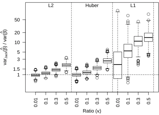
Empirical findingsAs in the pairs bootstrap case, simulations show that confidence intervals based on the jackknife estimate of variance lead to extremely poor inference for β1 (Figure 1) and that the jackknife dramatically overestimates the variance ofβb1 (Figure 6). For L2
and Huber loss, the jackknife estimate of variance is 10-15% too large forp/n= 0.1, and for
● ● ● ● ● ● ● ● ● ● ● ● ● ● ● ●● ● ● ● ● ● ● ● ● ● ●● ● ● ● ● ● ● ● ● ● ● ● ● ● ● ● ● ● ● ● ● ● ● ● ● ● ● ● ● ● ● ● ● ● ● ● ● ● ● ● ● ● ● ● ● ● ● ● ● ● ● ● ● ● ● ● ● ● ● ● ● ● ● ● ● ● ● ● ● ● ●
Ratio (κ)
v
a
rJa
c
k
(
β
^ ) / v
ar( β ^ ) 1 1.5 3 5 10 20 50
0.01 0.1 0.3 0.5 0.01 0.1 0.3 0.5 0.01 0.1 0.3 0.5
L2 Huber L1
Figure 6: Factor by which jackknife over-estimates the variance: boxplots of the ratio of the jackknife estimate of the varianceβb1to the variance ofβb1 as calculated
over 1000 simulations. Simulations were with normal design matrixXand normal error i with values of n = 500. Note that because the L1 jackknife estimates so wildly overestimate the variance, in order to put all the methods on the same plot the boxplot of ratio is on log-scale; y-axis labels give the corresponding ratio to which the log values correspond. For the median values of each boxplot, see Table A-6 in AppendixI.
2005). Even for p/n = 0.01, the estimate is not unbiased for L1, with median estimates twice as large as they should be and enormous variance in the estimates of variance. Higher dimensions only worsen the behavior with jackknife estimates being 15 times larger than they should.
4.1 Theoretical Results
Again, in the case of least-squares regression with a Gaussian design matrix, we can theo-retically evaluate the behavior of the jackknife. The proof of the following theorem is given in AppendixG (when the observations have covariance Id) and in AppendixH (to show how to extend the results to general covariance).
Theorem 3 Let us call varJ ACK the jackknife estimate of variance of v0βb given in (7), where v is any deterministic vector with kvk2 = 1. Suppose the design matrix X is such
that Xi iid
v N(0,Σ), βb is computed using least-squares, and the errors have a variance. Then we have, asn, p→ ∞ and p/n→κ <1,
E(varJ ACK)
var
v0βb
→
As in Theorem 2, the proof of Theorem 3 is based on random matrix techniques where further technical work should allow an extension for the entries of Xi,j to be i.i.d. from a
distribution other than Gaussian, providedXi,j’s have sufficiently many moments. This is
also beyond the scope of our work, but interested readers can see AppendixG.3 for more details.
Correcting the Jackknife in Least Squares Theorem 3 implies that scaling the jackknife estimate of variance by multiplying it by 1−p/nwill result in an estimate of var
b β1
with the correct expectation; simulations shown in Figure 7 confirm that confidence intervals based on this corrected estimate of variance yield correct confidence intervals for least-squares estimates ofβbwhen the design matrix X is Gaussian. However this scaling factor
is not robust to violations of these assumptions. In particular when the X matrix follows an elliptical distribution the correction of 1−p/n from Theorem 3 gives little improvement even when the loss is still L2 (Figure 7).
Corrections for more general settings For the more general setting of an elliptical design matrixX and loss functionρ, preliminary computations suggest an alternative result. Let
S be the random matrix defined by
S= 1
n n X
i=1
ψ0(ei)XiXi0.
Then in our asymptotic regime, and when Σ = Idp, preliminary heuristic calculations
suggest that we can estimate the amount by whichE(varJ ACK) overestimates the variance
of βb1 by E(ˆγ), where
ˆ
γ , trace S
−2 /p
[trace (S−1)/p]2 . (8) Note that when applied to least-squares regression with X ∼ N(0, Idp) this conforms
to our result in Theorem 3. Theoretical considerations suggest that in our asymptotics, for smooth ρ, ˆγ ' E(ˆγ), which suggests a data-driven correction to the jackknife estimate of variance; however that correction depends having information about the distribution of the design matrix.
Equation (8) assumes that the loss function can be twice differentiated, which is not the case for either Huber orL1 loss. In the case of non-differentiable ρ and ψ, we can use appropriate regularizations to make sense of those functions. Forρ= Huberk, i.e., a Huber
function that transitions from quadratic to linear at |x| = k, ψ0 should be understood as
ψ0(x) = 1|x|≤k. ForL1 loss, ψ0 should be understood as ψ0(x) = 1x=0.
In Figure 7 we show simulation results for confidence intervals created based on rescaling the jackknife estimate of variance by E(ˆγ) defined in Equation (8). In the case of least-squares with an elliptical design matrix, this correction—which directly uses the distribution of the observed X matrix—leads to a definite improvement in our jackknife confidence intervals. Similarly, for the Huber loss we see a definite improvement as compared to the standard jackknife estimate, as well as an improvement over the simpler correction of 1−p/n
that would be appropriate for squared error loss.