Cube Attacks
Chen-Dong Ye and Tian Tian
PLA Strategic Support Force Information Engineering University, 62 Kexue Road, Zhengzhou, 450001, China. [email protected],[email protected]
Abstract.Cube attacks are an important type of key recovery attacks against NFSR-based cryptosystems. The key step in cube attacks closely related to key recovery is recovering superpolies. However, in the previous cube attacks including original, division property based, and correlation cube attacks, the algebraic normal form of superpolies could hardly be shown to be exact due to an unavoidable failure probabil-ity or a requirement of large time complexprobabil-ity. In this paper, we propose an algebraic method aiming at recovering the exact algebraic normal forms of superpolies practi-cally. Our method is developed based on degree evaluation method proposed by Liu in Crypto-2017. As an illustration, we apply our method to Trivium. As a result, we recover the algebraic normal forms of some superpolies for the 818-, 835-, 837-, and 838-round Trivium. Based on these superpolies, on a large set of weak keys, we can recover at least five key bits equivalently for up to the 838-round Trivium with a complexity of about237. Besides, for the cube proposed by Liu in Crypto-2017 as a zero-sum distinguisher for the 838-round Trivium, it is proved that its superpoly is not zero-constant. Hopefully, our method would provide some new insights on cube attacks against NFSR-based ciphers.
Key Words: Trivium, cube attacks, key recovery attacks, algebraic normal form
Keywords: No keywords given.
1
Introduction
The cube attack was first proposed by Dinur and Shamir at Eurocrypt-2009 in [1]. Lat-er, there were many improvements on it such as cube testers [2], dynamic cube attacks [3], conditional cube attacks [4], division property based cube attacks [5, 6] and correla-tion cube attacks [7]. Due to these improvements, cube attacks have become more and more powerful. In particular, it is one of the most important cryptanalytic tools against Trivium.
In the original cube attacks [1, 8, 9, 10], the main aim is to find low-degree super-polies on key variables by performing experimental tests. In [1], the authors recovered35 linear superpolies of the 767-round Trivium. In [8], quadraticity tests were first applied
to the cube attacks against Trivium. As a result, the authors found 41 linear and 38
quadratic superpolies for the 709-round Trivium. In [9], the authors proposed two new ideas concerning cube attacks against Trivium. One was a recursive method to construct useful cubes. The other was simultaneously testing a lot of subcubes of a large cube using
the Meobius transformation. They found 12 linear and 6 quadratic superpolies for the
ones, while testing cubes of size greater than 35 is time consuming. Hence, the sizes of cubes are typically confined to 40.
In [5], Todo et al. introduced division property to cube attacks. For a cubeI, by solving the corresponding mixed integer linear programming (MILP) models built according to the propagation rules of division property, they could identify a set of key variables which
includes the key variables appearing in the superpoly pI. Then, by constructing the
truth tables of pI corresponding to randomly chosen assignments of non-cube variables,
they attempted to find a proper one ensuring that pI was non-constant. Finally they
recoveredpI by its truth table. Due to division property and the power of MILP solvers, large cubes could be explored. For example, in [5], it was shown that the superpoly of a given 72-dimensional cube was dependent on at most five key variables for the 832-round Trivium. In [6], the authors improved the work in [5] in finding a proper non-cube variables assignment and reducing the complexity of recovering the superpoly. It was shown in [6] that the superpoly of a given 78-dimensional cube was dependent on at most one key variable for the 839-round Trivium. For division property based cube attacks, the advantage is that large cubes could be explored and the complexity of recovering superpolies could be estimated theoretically. The implicit disadvantage is that the theory of division property could not ascertain that a superpoly for a cube is non-constant. Hence the key recovery attacks on the 832-round Trivium in [5] and on the839-round Trivium in [6] are only possible which may be only a distinguisher.
In [11], the authors proposed a method to recover the superpoly of a cube with the help of bit-based division property. According to the results of [11], the superpoly of the cube proposed in [6] to attack the 839-round Trivium is zero-constant. Besides, for the cube given in [5] to attack the 832-round Trivium, they found an assignment to noncube IV variables which ensures the corresponding superpoly is non-constant. However, the complexity of the method proposed in [11] largely depends on the number of key variables appearing in the superpoly, and so it is not suitable to recover superpolies which include many key variables. Furthermore, in [11], the authors did not establish new attacks on Trivium variants with more than 832 initialization rounds.
In [7], the authors proposed the correlation cube attacks. For a cubeCI, the authors first tried to find a set of low-degree polynomialsG, called a basis, such that the superpoly
pI could be factored intopI =
⊕
g∈Gg·fg formally. Then, by exploiting the correlation
relations between the low-degree basisGand the superpolypI, they could obtain a set of
probabilistic equations on the secret key variables since fg is unknown. It was reported
in [7] that five key variables of the835-round Trivium could be recovered with244 time
complexity,245keystream bits, and 251 preprocessing time.
In [12], Fu et al. gave a dedicated attack on the 855-round Trivium which somewhat resembled dynamic cube attacks. Their main idea is finding a simple polynomialP1 such that the output bit polynomialz could be formally represented as z=P1P2⊕P3 where
P2 is complex while P3 is a low-degree polynomial on IV variables compared with z.
Consequently, (P1⊕1)z = (P1⊕1)P3 will be a low-degree polynomial on IV variables.
Then they guessed some secret key expressions involved in P1. For a group of right
guesses,(P1⊕1)zwill be a low-degree polynomial on IV variables. Otherwise,(P1⊕1)zis
expected to be a high-degree polynomial. They declared that three secret key bits could be recovered for the 855-round Trivium with the online complexity of274. A shortage of
the attack described in [12] is that no estimation was given on the successful probability for wrong guesses.
1.1
Our Contributions.
In this paper, we propose an algebraic method to recover superpolies in cube attacks, which improves the original cube attacks in recovering the superpolies with proved correctness and overcoming the low-degree restriction.
The basic idea of our attacks is, by making use of internal state bit variabless(r1)=
(s(r1) 1 , s
(r1) 2 , . . . , s
(r1)
N ), dividing the polynomial representation fr(key,iv) of an r-round
cipher into an r1-round polynomial representation s(r1)(key,iv) and an r2-round
poly-nomial representation gr2(s(r1)) such that fr = gr 2(s
(r1)(key,iv)). Then it is possible
for us to compute superpolies algebraically for a class of cubes which are called useful cubes in the rest of this paper. The criterion of a useful cube plays a key role in calculat-ing superpolies in practice. In particular, for a useful cubeI, to compute the superpoly
Q {s(r1 )
i1 ,s (r1 )
i2 ,...,s (r1 )
il }
of I in the polynomial s(r1)i1 (key,iv)s(r1)i2 (key,iv)· · ·s(r1)i
l (key,iv) for
a term s(r1)i 1 s
(r1) i2 · · ·s
(r1)
il appearing in the algebraic normal form of gr2(s
(r1)), it is only
necessary to know themaximum degree termsin eachs(r1)
ij (key,iv)for1≤j≤l. Hence a
superpolyQ
{s(r1 )
i1 ,s (r1 )
i2 ,...,s (r1 )
il }
could be computed in practice and so is the targeted
super-polypI in fr(key,iv)which is equal to the summation of all possibleQ{s(r1 )
i1 ,s (r1 )
i2 ,...,s (r1 )
il }
.
As an illustration, we apply our method to the round-reduced Trivium, and we obtain the following results.
• For Trivium variants with 800-832 initialization rounds, we randomly test 10000
cubes of size 33-36, and obtain about 175 useful cubes for each variant in average. This indicates that useful cubes exist widely.
• We recover the superpolies of some useful cubes for the818-, 835-, 837-, and 838-round Trivium. With these recovered superpolies, we could establish the following attacks.
- For the 818-round Trivium, we could recover at least 10 key bits equivalently on about270 weak keys;
- For the 835-round Trivium, we could recover at least 12 key bits equivalently on about267 weak keys;
- For the 837-round Trivium, we could obtain 5 deterministic and 2 probabilistic equations on about272.20weak keys;
- For the 838-round Trivium, we could obtain 5 deterministic and 2 probabilistic equations on about271.75weak keys.
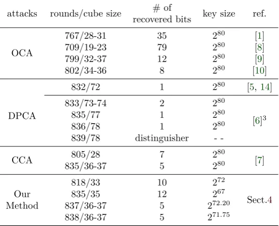
We further compare our attacks with the original cube attacks (OCA), the division property based cube attacks (DPCA), and correlation cube attacks (CCA). First, our attacks can recover the superpoly exactly. Second, we can attack Trivium variants with high rounds using cubes of relative small sizes, i.e., we can reach the 838-round Trivium with cubes of sizes 36-37. Compared with original cube attacks, we can improve more than 30 rounds at the cost of increasing the sizes of cubes slightly. In division property based cube attacks, they need cubes of sizes over70to attack Trivium variants with more than 830 initialization rounds. Besides, since it can not ensure that the superpoly of a cube is non-constant in division property based cube attacks, the attacks in [5,14,6] may be only distinguishing attacks. In correlation cube attacks, they can attack the 835-round Trivium with cubes of sizes 36-37, but they can not recover the exact superpoly of a cube and the correlation probability is computed experimentally. We summarise these comparisons in Table 1, where the “key size” column lists the size of keys which are vulnerable to each attack.
3The attacks proposed in [6] against the 833-, 835- and 836-round Trivium may be only distinguishing
Table 1: Comparison with previous cube attacks
attacks rounds/cube size # of key size ref.
recovered bits
OCA
767/28-31 35 280 [1]
709/19-23 79 280 [8]
799/32-37 12 280 [9]
802/34-36 8 280 [10]
DPCA
832/72 1 280 [5,14]
833/73-74 2 280
[6]3
835/77 1 280
836/78 1 280
839/78 distinguisher
-CCA 805/28 7 2
80
[7]
835/36-37 5 280
818/33 10 272
Sect.4
Our 835/35 12 267
Method 837/36-37 5 272.20
838/36-37 5 271.75
1.2
Organization
The rest of this paper is organized as follows. In Section 2, we give some necessary introductions on cube attacks, the Numeric Mapping method, and the IV Representation techniques. In Section3, we show the general idea of our attacks. In Section4, we apply our attacks to Trivium. Finally, Section5concludes this paper.
2
Preliminaries
2.1
Boolean Functions and Algebraic Degree.
A Boolean function onnvariables is a mapping fromFn
2 toF2, whereF2is the finite field
of two elements and Fn
2 is ann-dimensional vector space over F2. A Boolean functionf
can be represented by a polynomial on nvariables overF2,
f(x1, x2, . . . , xn) = ⊕
c=(c1,c2,...,cn)∈Fn2 ac
n
∏
i=1 xci
i ,
which is called the algebraic normal form (ANF) off. In this paper,u=ac
∏n i=1x
ci
i (ac̸=
0)is called a term of f. The algebraic degree of a Boolean function is denoted bydeg(f) and defined as
deg(f) =max{wt(c)|ac ̸= 0},
wherewt(c)is the Hamming Weight ofc. In this paper, we also care about the algebraic degree off on a subsetI of{x1, x2, . . . , xn}, which is denoted bydegI(f)and defined as
degI(f) =max{wtI(c)|ac̸= 0},
Algorithm 1Pseudo-code of Trivium
1: (s1, s2, . . . , s93)←(k0, k1, . . . , k79,0, . . . ,0);
2: (s94, s95, . . . , s177)←(v0, v1, . . . , v79,0, . . . ,0);
3: (s178, s179, . . . , s288)←(0, . . . ,0,1,1,1);
4: forifrom 1 toN do
5: if i >1152then
6: zi−1152←s66⊕s93⊕s162⊕s177⊕s243⊕s288;
7: end if
8: t1←s66⊕s91·s92⊕s93⊕s171;
9: t2←s162⊕s175·s176⊕s177⊕s264;
10: t3←s243⊕s286·s287⊕s288⊕s69;
11: (s1, s2, . . . , s93)←(t3, s1, . . . , s92);
12: (s94, s95, . . . , s177)←(t1, s94, . . . , s176);
13: (s178, s179, . . . , s288)←(t2, s178, . . . , s287);
14: end for
2.2
Description of Trivium
Trivium is a bit oriented synchronous stream cipher designed by Cannière and Preneel, which is one of eSTREAM hardware-oriented portfolio ciphers. It accepts an 80-bit key and an 80-bit initialization vector. For a more detailed and formal description, we refer the reader to [15].
The main building block of Trivium is a288-bit Galois nonlinear feedback shift register with three registers. In every clock cycle, there are three bits of the internal state updated by quadratic feedback functions and all the other bits of the internal state are updated by shifting. The internal state of Trivium, denoted by (s1, s2, . . . , s288), is initialized by loading an 80-bit secret key and an 80-bit IV into the registers, and setting all the remaining bits to 0 except for the last three bits of the third register. Then, the algorithm would not output any keystream bit until the internal state is updated 1152rounds, see Algorithm1 for details.
2.3
Superpoly.
The concept of superpoly was first proposed in [1]. Letf(x1, x2, . . .,xm)be anm-variable
polynomial and I = {xi1, xi2, . . . , xid} be a subset of {x1, x2, . . . , xm}. Denote tI =
∏d
j=1xij, the product of variables inI. Then it is clear that the following representation
f =f1·tI +f2
for f is unique, wheref1 does not contain any common variable with tI and every term in f2 is not divisible bytI. The polynomialf1is called thesuperpoly oftI inf. For the sake of convenience, we denotef1 by tf
I in the following paper.
2.4
Cube Attacks.
The idea of cube attack was first proposed by Dinur and Shamir in [1]. In the cube attack against stream ciphers, an output bitz is described as a tweakable polynomialf on key variables key= (k0, k1, . . . , kn−1) and public IV variablesiv= (v0, v1, . . . , vm−1), where nandmare positive integers, i.e.,
Let I be a subset containingd public variables called cube variables, where1≤d≤m. Without loss of generality, we assume that I={v0, v1, . . . , vd−1}. Let us denote
pI(key) = f
tI, (1)
the superpoly oftI inf under the condition that allmIV variables are set to0except the d variables inI. LetCI be a set of assignments for IV variables containing 2d m-tuples
in which the variables in I are assigned to all the possible combinations of 0/1while all the other IV variables, called non-cube IV variables, are assigned to constants. The set
CI is called ad-dimensional cube defined byI. In this paper, we set all the non-cube IV variables to 0’s and callI a cube for simplicity. A key observation in cube attacks is that the summation off over all the2d possible vectors in CI leads topI, i.e.,
pI(key) = ⊕
v∈CI
f(key,v). (2)
If pI(key) is not a constant polynomial, then this means that by choosing IVs, one can obtain an equation in key variables. Otherwise, (2) provides a distinguisher on the ci-pher. Hence an attacker in cube attacks focuses on recovering pI(key). Because f is
treated as a black-box polynomial, in practice pI is not algebraically calculated from (1).
Hence, original cube attacks resort to low-degree polynomial tests with a certain failure probability.
2.5
The Numeric Mapping.
The numeric mapping was firstly introduced by Liu in [16], which was the core technique of the degree evaluation method for NFSR-based cryptosystems in [16]. Let
f(x1, x2, . . . , xm) =
⊕
c=(c1,c2,...,cm)∈Fm2 ac
m
∏
i=1 xci
i
be an m-variable Boolean function. The numeric mapping, denoted byDEG, is defined
as follows
DEG :Bm×Zm→Z
(f, D)7→maxac̸=0
m
∑
i=1 cidi,
whereD= (d1, d2, . . . , dm),Bmis the set of allm-variable Boolean functions.
With the numeric mapping, the numeric degree of a composite function can be defined. Assume that g1, g2, . . . , gmare n-variable Boolean functions and h=f(g1, g2, . . . , gm) is
a composite function. The numeric degree of h is defined as DEG(f,deg(G)), where
G = (g1, g2, . . . , gm) and deg(G) = (deg(g1),deg(g2), . . . ,deg(gm)). Furthermore, if we
have deg(gi)≤di for1≤i≤m, then it can be seen that
deg(h)≤DEG(f,deg(G))≤DEG(f, D)
whereD= (d1, d2, . . . , dm).
2.6
The IV Representation.
The IV representation was first proposed by Fu et al. in [17], which was used to determine the nonexistence of some IV terms in the output bit of Grain-128. For a stream cipher with m IV variables, i.e., v0, v1, . . . , vm−1, and n key variables, i.e., k0, k1, . . . , kn−1, an
internal state bit (or the output bit)scan be seen as a polynomial on key and IV variables, i.e.,
s=f(key,iv) =⊕
I,J
∏
vi∈I
vi ∏ kj∈J
kj.
The IV representation of a termu=∏v
i∈Ivi
∏
kj∈Jkjis defined asuIV =
∏
vi∈Ivi.Based
on the definition of IV representation of a term, the IV representation ofs is defined as follows,
sIV =∑
I
∏
vi∈I
vi.
3
An Algebraic Method to Recover Superpolies
Recall that in an original cube attack, a desirable superpoly is not algebraically computed from (1), since the output bit polynomial is treated as a black-box polynomial. Hence original cube attacks resort to low-degree polynomial tests such as BLR linearity tests with a certain failure probability. Consequently, previously recovered superpolies in original cube attacks are convincing but without proved correctness. In this section, we shall give an algebraic method to recover superpolies in cube attacks against an NFSR-based stream cipher.
In Subsection3.1, we describe the rationality of our idea and the general framework for realizing the idea. Then to make our idea practical, we introduce a new criterion of useful cubes in Subsection 3.2. Consequently, an algorithm is proposed to find useful cubes efficiently in Subsection 3.3. Finally, in Subsection3.4, for a useful cube, we show how to recover its superpoly as well as some auxiliary techniques.
3.1
An Overview of Our Method
We represent the superpoly of a cube by internal state bits for the target cipher. Let us fix a time instancet≥0which is less than the number of initialization rounds and denote the internal state bits of the target cipher at the time instancetbys= (s(t)1 , s(t)2 , . . . , s(t)N ), whereN is the internal state size of the target cipher. Then an output bitz of the target cipher also can be described by a polynomial ons= (s(t)1 , s(t)2 , . . . , s(t)N ), i.e.,
z=gt(s(t)1 , s(t)2 , . . . , s(t)N) = ⊕
c=(c1,c2,...,cN)∈FN2 ac
N
∏
i=1
(s(t)i )ci, (3)
where ac ∈ {0,1}. Furthermore, note that each internal state bits (t)
i (1≤i≤N)could
be represented by a polynomial on key and IV variables, i.e.,
s(t)i =s(t)i (key,iv). (4)
Taking (4) into (3) yields
Following from (5), the superpoly ofI inz can be computed as
pI = gt(s
(t)
1 (key,iv), s (t)
2 (key,iv), . . . , s (t)
N (key,iv)) tI
=
⊕
c=(c1,c2,...,cN)∈FN2
ac∏Ni=1(s(t)i (key,iv))ci
tI
= ⊕
c=(c1,c2,...,cN)∈FN2 ac=1
ac
∏N i=1(s
(t)
i (key,iv)) ci
tI . (6)
For the sake of convenience, we simply denotes(t)i (key,iv)bys(t)i in the rest of the paper. Then (6) implies that
pI = ⊕
c=(c1,c2,...,cN)∈FN2 ac=1
ac
∏N i=1(s
(t) i )
ci
tI . (7)
Note thatac∏Ni=1(s(t)i )ci withac = 1is a term ofgt. If we denote all terms ofgtbyT(gt),
i.e.,
T(gt) ={ac N
∏
i=1
(s(t)i )ci|a
c = 1, c= (c1, c2, . . . , cN)∈FN2},
then it follows from (7) that
pI = ⊕
s(it) 1s
(t)
i2···s (t)
il∈T(gt)
s(t)i 1 s
(t) i2 · · ·s
(t) il
tI . (8)
This indicates that if we could compute the superpoly oftI ins(t)i1s(t)i2 · · ·s(t)il for every term
s(t)i1 s(t)i2 · · ·s(t)i
l of gt, then their summation is the desirable superpolypI in cube attacks.
In the following paper, we shall recoverpI based on the equality (8). Hence it is clear
that the superpolies recovered with our method will be correct with probability 1. In specific, for a given set I of cube variables and a time instance t, there are three main steps:
• Step 1. Compute the ANF ofgt.
• Step 2. For each terms(t)i1 s(t)i2 · · ·s(t)i
l ∈T(gt), compute the superpoly
Q{s(t)
i1,s (t)
i2,...,s (t)
il}
=s
(t) i1s
(t) i2 · · ·s
(t) il
tI .
• Step 3. Compute
pI =
⊕
s(it) 1s
(t)
i2···s (t)
il∈T(gt)
Q {s(it)
1,s (t)
i2,...,s (t)
il}
.
Rule 1 One can compute the ANF of gt(s(t)1 , s2(t), . . . , s(t)N ), where s(t)i is treated as a
bit variable. Astdecreases, the ANF of gt(s1(t), s(t)2 , . . . , s(t)N)will become more and more complex.
Rule 2 Fori from 1 to N, one can compute the ANF of s(t)i (key,iv). As t increases, the ANF ofs(t)i (key,iv)will become more and more complex.
Third, we point out that to computeQ
{s(it) 1,s
(t)
i2,...,s (t)
il}
is a difficult problem in this
frame-work even when the above two rules are satisfied, since it is difficult to compute the complete ANF of the product s(t)i1s(t)i2 · · ·s(t)i
l when treating s
(t)
ij as a polynomial on key
and IV variables. To solve this problem, in Subsection 3.2, we give a criterion to choose
useful cubes for which we could computeQ
{s(it) 1,s
(t)
i2,...,s (t)
il}
in practice without completely
expanding the products(t)i 1 s
(t) i2 · · ·s
(t)
il in its ANF.
3.2
A New Criterion of Useful Cubes
Let Q
{s(it) 1,s
(t)
i2,...,s (t)
il}
be as in the previous subsection. To compute Q
{s(it) 1,s
(t)
i2,...,s (t)
il}
, we
use the following expression
Q{s(t)
i1,s (t)
i2,...,s (t)
il}
=⊕t1t2· · ·tl
tI , (9)
where tj runs throughT(s(t)i
j )independently for 1 ≤j ≤l. The difficulty of computing
(9) lies in that there are too many products, sayt1t2· · ·tl, need to compute. Ift1t2· · ·tl
is not divisible bytI, then we have
t1t2· · ·tl tI = 0,
which implies that t1t2· · ·tl has no contribution to Q{s(t)
i1,s (t)
i2,...,s (t)
il}
. Hence an effective
t1t2· · ·tl should satisfy that t1t2· · ·tl is divisible by tI. To make this point clear we rewrite (9) as
Q{s(t)
i1,s (t)
i2,...,s (t)
il}
= ⊕
tI|t1t2···tl
t1t2· · ·tl tI
, (10)
where tj runs through T(s(t)i
j ) independently for 1 ≤ j ≤ l. To reduce the number
of effective terms or summation in (10) we propose a criterion for useful cubes in this subsection.
To characterize a useful cube, we shall give some definitions first.
Definition 1. LetIbe a set of cube variables,t≥0, and1≤i≤N. If a termu∈T(s(t)i ) satisfiesdegI(u) = degI(si(t)), thenuis called a maximum degree term ofs(t)i onI.
A maximum degree term of s(t)i on I is a term whose degree on I attains the max-imum. It is obvious that a maximum degree term of s(t)i is not unique. For example,
I = {v1, v2, v3, v4} and s(t)i =v1v2k1⊕v2v3k1k2⊕v4k3. Then v1v2k1 and v2v3k1k2 are maximum degree terms ofs(t)i whose degrees onI are 2.
Definition 2. LetI be a set of cube variables andt≥0. For a termu=∏lj=1s(t)ij , if
l
∑
j=1
degI(s(t)i
j ) =|I|,
The following property gives a relationship between tight terms and maximum degree terms concerning the right hand side of (10).
Property 1. LetI be a set of cube variables andu=s(t)i1s(t)i2 · · ·s(t)il be a tight term for
I. Ift1t2· · ·tl is divisible bytI where tj ∈ T(s (t)
ij )for 1 ≤j ≤l, then tj is a maximum
degree term of s(t)ij onI.
Lets(t)i1s(t)i2 · · ·s(t)i
l be a tight term forI. Due to Property1, when computing
s(it) 1s
(t)
i2···s (t)
il
tI ,
we only need to consider maximum degree terms of s(t)i
j onI. Moreover, maximum
de-gree terms are usually a very small part of s(t)ij . Thus, in this case the computation of
s(it) 1s
(t)
i2···s (t)
il
tI could be simplified greatly.
Example 1. Let I = {v0, v1, v2, v3}, s1 = v0v1k0 ⊕v2 ⊕v3, s2 = v2v3k5⊕v0⊕v2,
s3 =v2⊕v3, u1 =s1s2, andu2=s2s3. Then it can be seen that u1 is a tight term for
I. However,u2is not a tight term forI. The sets of maximum degree terms of s1ands2
are{v0v1k0} and{v2v3k5}, respectively. According to Property1, we have u1
tI =k0k5,
which could be computed only using the maximum degree terms of s1ands2.
Based on the concept of tight terms, we propose a new criterion of useful cubes.
Criterion 1. Let Ibe a set of cube variables andz=gt(s (t) 1 , s
(t) 2 , . . . , s
(t)
N). If every term u=s(t)i
1s (t) i2 · · ·s
(t)
il ∈T(gt)satisfies
l
∑
j=1
degI(s(t)i
j )≤ |I|, (11)
thenI is called a useful cube.
In Criterion1, if∑lj=1degI(s(t)i
j ) =|I|, then s
(t) i1s
(t) i2 · · ·s
(t)
il is a tight term ofgt forI;
otherwise we have
l
∑
j=1
degI(s(t)i
j )<|I|
which implies thats(t)i 1 s
(t) i2 · · ·s
(t)
il is not divisible bytI, and so
s(t)i 1 s
(t) i2 · · ·s
(t) il
tI = 0.
Therefore, this criterion implies that every termuof gtis either a tight term or tu
I = 0.
Accordingly for a useful cubeI, we simply have
pI =
⊕
s(it) 1s
(t)
i2···s (t)
il
is a tight term ofgt
Q {s(it)
1,s (t)
i2,...,s (t)
il}
= ⊕
s(it) 1s
(t)
i2···s (t)
il
is a tight term ofgt
⊕
tjis a maximum
degree term ofs(t)
ij
t1t2· · ·tl tI
. (12)
Algorithm 2Finding Useful Cubes with Degree Evaluation
Require: the chosen cube variablesI, the chosen time instancet
1: Express the output bitz asz=gt(s(t));
2: Iteratively calculateDEGI(s (t)
i )fori∈ {1,2, . . . , N};
3: foreach termu=s(t)i 1s
(t) i2 · · ·s
(t)
il ofgtdo
4: SetDEGI(u) =
∑l
j=1DEGI(s (t) ij );
5: if DEGI(u)>|I| then
6: return useless;
7: end if
8: end for
9: return useful;
3.3
An Algorithm to Find Useful Cubes
In this subsection, we discuss how to find useful cubes efficiently. According to Rule 1, we assume thatgt is known, and soT(gt)is known. It can be seen from Criterion1that
to judge whetherI is useful we need to calculate
l
∑
j=1
degI(s(t)i
j )
for every terms(t)i1 s(t)i2 · · ·s(t)i
l inT(gt). This is in essence a degree evaluation problem. On
one hand, to quickly judge whether a cube is useful, we need an efficient degree evaluation algorithm. On the other hand, to accurately identify a useful cube, we need an accurate degree evaluation algorithm since a useful cube may be missed if the estimated degrees are far from real degrees. Considering these issues, we choose to use the idea of numeric mapping proposed in [16]. Details are given in Algorithm 2. As for the definition and methodology of numeric mapping and numeric degree please refer to [16] and Section2.
The general idea of Algorithm2is first computing the numeric degree ofs(t)i onI for 1≤i≤N denoted by DEGI(s
(t)
i )and then computing the numeric degree for each term
s(t)i 1 s
(t) i2 · · ·s
(t)
il ∈T(gt)by
DEGI(s (t) i1 s
(t) i2 · · ·s
(t) il ) =
l
∑
j=1
DEGI(s (t) ij ).
If
DEGI(s (t) i1 s
(t) i2 · · ·s
(t) il )≤ |I|
holds for every terms(t)i 1 s
(t) i2 · · ·s
(t)
il ∈T(gt), then we regardIas a useful cube in Algorithm
2. Since the algebraic degree of s(t)i is always less than or equal to the numeric degree of s(t)i , i.e., degI(s(t)i ) ≤ DEGI(s
(t)
i ), it follows that a cube outputted by Algorithm 2
satisfies Criterion1.
3.4
Recover the Exact Superpoly of a Useful Cube
After finding a useful cubeI, we can recover the corresponding superpolypI by (12). The critical part of this phase is calculating the superpoly oftI in each tight term forI. We present the details in Algorithms 3and4.
Letu=s(t)i 1s
(t) i2 · · ·s
(t)
il be a tight term forI. In Algorithm3, the procedure
Recover-Coefficient is called to computeQ{s(t)
i1,s (t)
i2,...,s (t)
il}
. Following from (12),Q{s(t)
i1,s (t)
i2,...,s (t)
is the summation of
t1t2· · ·tl tI
,
where t1t2· · ·tl is divisible by tI and tj is a maximum degree term of s(t)i
j for j ∈
{1,2, . . . , l}. Hence, we need to find all such products of maximum degree terms of
s(t)i 1 , s
(t) i2, . . . , s
(t)
il to obtain Q{s(it) 1,s
(t)
i2,...,s (t)
il }
. In RecoverCoefficient, it can be done in
the following three steps.
Collect and Preprocess the Maximum Degree Terms. The first step is to collect and preprocess the maximum degree terms of s(t)i
j forj ∈ {1,2, . . . , l}. Assume that the
maximum degree terms of s(t)i
j are stored in M DT[j], where M DT is a list of sets and
M DT[j]represents thej-th set inM DT. Our goal is to find all the combinations
(t1, t2, . . . , tl)∈M DT[1]×M DT[2]× · · · ×M DT[l]
such that∏lj=1tj is divisible bytI. Let t′j be the IV representation oftj for 1≤j ≤l.
Then, if∏lj=1tjis divisible bytI, then
∏l
j=1t′j=tI (the IV variables except cube variables
are set to 0). Therefore, we apply theReduce operation toM DT[j]for1≤j ≤l. In the
Reduceoperation, we first do IV representation for each term inM DT[j], and so we could obtain a multi-setV M DT[j] ={uIV|u∈M DT[j]}, where uIV is the IV representation of u. Then, we could obtain a set RM DT[j] from V M DT[j], where only one of the repeated terms inV M DT[j]are kept. For simplicity,RM DT[j]is called a set of reduced maximum degree terms in the rest of this paper.
In this paper, a combination
(t1j1, t 2 j2, . . . , t
l
jl)∈RM DT[1]×RM DT[2]× · · · ×RM DT[l]
satisfying∏li=1ti
ji =tI is called a valid combination. It can be seen that, by finding all
the valid combinations, we could deduce all the combinations
(t1, t2, . . . , tl)∈M DT[1]×M DT[2]× · · · ×M DT[l]
such that ∏li=1ti is divisible bytI. Note that ∏li=1|RM DT[i]| would be much smaller than∏li=1|M DT[i]|, sinceM DT[i](1≤i≤l) may have many terms whose results of IV representation are the same. Thus, the complexity could be reduced dramatically.
Find All the Valid Combinations. Accordingly, the second step is to find all the valid combinations. Although∏li=1|RM DT[i]|would be much smaller than∏li=1|M DT[i]|, it may still be very large. Hence, we would not check each combination (t1
j1, t 2 j2, . . . , t
l jl)
directly, whereti
ji ∈RM DT[i]for1≤i≤l. Instead, we pick up elements fromRM DT
gradually to form a full combination. Moreover, we propose the following two strategies to throw away some invalid combinations in advance. To illustrate these two strategies, assume that we have picked up the firstdelements of a combination, i.e.,t1
j1, t 2 j2, . . . , t
d jd.
Strategy 1. If degI(t1 j1· · ·t
d
jd) < degI(t
1
j1) +· · ·+ degI(t d
jd), then we would throw
away all the combinations whose firstdcomponents aret1 j1, t
2 j2, . . . , t
d jd.
Let(t1 j1, t
2 j2, . . . , t
d jd, t
d+1 jd+1, . . . , t
l
jl)be a combination such that the condition in Strategy
1 is satisfied. Then,
degI(t1j1· · ·tljl) ≤ degI(t1j1· · ·tdjd) + degI(td+1j
d+1· · ·t l jl)
< d
∑
i=1
degI(tij
i) + degI(t
d+1 jd+1· · ·t
l jl)
≤
l
∑
i=1
Namely,degI(t1 j1t
2 j2· · ·t
l
jl)<|I|. Hence, combinations satisfying the condition in Strategy
1 are not valid ones and should be thrown away.
Strategy 2. For some d+ 1 ≤ w ≤ l, if each term tw ∈ RM DT[w] satisfies that
degI(tw·t1j1t 2 j2· · ·t
d
jd)<degI(tw) + degI(t
1 j1t
2 j2· · ·t
d
jd), then we would throw away all the
combinations whose firstdcomponents aret1 j1, t
2 j2, . . . , t
d jd.
Let(t1 j1, t
2 j2, . . . , t
d jd, t
d+1 jd+1, . . . , t
l
jl)be a combination such that the condition in Strategy
2 is satisfied. Without loss of generality, we assume thatw=d+ 1. Then,
degI(t1j 1· · ·t
l
jl) ≤ degI(t
1 j1· · ·t
d+1
jd+1) + degI(t d+2 jd+2· · ·t
l jl)
< degI(t1j1· · ·tdj
d) + degI(t
d+1 jd+1)
+ degI(td+2j
d+2· · ·t l jl)
≤
l
∑
i=1
degI(tij
i) =|I|.
Namely,degI(t1j1t2j2· · ·tljl)<|I|. Hence, combinations satisfying the condition in Strategy 2 are not valid ones and should be thrown away.
If the chosen first d components do not satisfy the condition in Strategy 1 nor the condition in Strategy 2, then we would pick up the(d+ 1)-th component fromRM DT[d+ 1]. Note that, Strategies 1 and 2 can be applied again to judge whether the combinations which contain the chosen firstd+1components should be thrown away. Namely, Strategies 1 and 2 can be used again and again until a full combination is formed. Benefited from these two strategies, we can throw away many combinations in advance and the phase of finding all the valid combinations can be accelerated dramatically.
Recover the Superpoly of I in a Tight Term u. The final step is to recover the superpoly of I in u according to all the valid combinations. Let (t1
j1, t 2 j2, . . . , t
l jl)
be a valid combination. Since the terms in RM DT[i] are reduced from M DT[i], the combination (t1
j1, t 2 j2, . . . , t
l
jl)may correspond to several combinations(t1, t2, . . . , tl)such
that ∏lj=1tj is divisible bytI, where tj ∈M DT[j] for1 ≤j ≤l. All the combinations which(t1
j1, t2j2, . . . , tljl)corresponds to can be covered by a vector(λ
1
j1, λ2j2, . . . , λljl), where
λwjw =
s(t)i
w
tw jw
for w ∈ {1,2, . . . , l}. In this paper, (λ1j1, λ2j2, . . . , λljl) is called the superpoly vector of (t1j1, t2j2, . . . , tljl). Then, the contribution of the valid combination (t1j1, t2j2, . . . , tljl)to the superpoly ofI inuis∏lw=1λw
jw. Thus,
Q{s(t)
i1,s (t)
i2,...,s (t)
il}
= ⊕
(t1j 1,t
2
j2,...,t
l jl)is valid
l
∏
w=1 λwjw.
As an illustration of Algorithms3and4, we provide the following example.
Example 2. LetI={v0, v1, v2, v3, v4, v5, v6, v7, v8, v9}be a set of cube variables. Assume that u=s1s4s6s8, where
s1=v4v5k2k3⊕v4v5k4⊕v4v5k5⊕v2v3⊕v5v6⊕k3,
s4=v0v1v2v3k0⊕v0v1v2v3k1⊕v0v1v3v4k0⊕v0v1v4v6k2
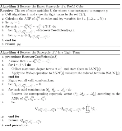
Algorithm 3Recover the Exact Superpoly of a Useful Cube
Require: The set of cube variablesI, the chosen time instancetto computegt
1: Call Algorithm2, and store the tight terms in the setT(I);
2: Calculate the ANF ofs(t)i on cube and key variables fori∈ {1,2, . . . , N};
3: SetpI = 0;
4: foreachu=s(t)i 1s
(t) i2 · · ·s
(t)
il ∈T(I)do
5: SetQ{s(t)
i1,s (t)
i2,...,s (t)
il}
=RecoverCoefficient(u,I);
6: SetpI =pI⊕Q{s(t)
i1,s (t)
i2,...,s (t)
il}
;
7: end for
8: return pI;
Algorithm 4Recover the Superpoly ofI in a Tight Term
1: procedure RecoverCoefficient(u,I)
2: Assume thatu=s(t)i1s(t)i2 · · ·s(t)i
l ;
3: for1≤j≤l do
4: Collect maximum degree terms ofs(t)ij and store them inM DT[j];
5: Apply theReduceoperation toM DT[j]and store the reduced terms inRM DT[j];
6: end for
7: Figure out all valid combinations;
8: SetQ {s(it)
1,s (t)
i2,...,s (t)
il}
= 0;
9: foreach valid combination(t1j1, t2j2, . . . , tljl)do
10: Recover the corresponding superpoly vector (λ1j1, λ2j2, . . . , λljl) according to the ANFs ofs(t)i
1, s (t) i2, . . . , s
(t) il ;
11: Set
Q{s(t)
i1,s (t)
i2,...,s (t)
il}
=Q{s(t)
i1,s (t)
i2,...,s (t)
il}⊕
l
∏
w=1 λwjw;
12: end for
13: return Q{s(t)
i1,s (t)
i2,...,s (t)
il}
;
14: end procedure
s6=v3v6⊕v4v6⊕v6v7, ands8=v6v9⊕v7v9⊕v8v9.
The first step is to collect the reduced maximum degree terms. It can be obtained that the set of maximum degree terms ofs1 is
M DT[1] ={v4v5k2k3, v4v5k4, v4v5k5, v2v3, v5v6}.
Then, the Reduce operation is applied. After applying the IV representation, we could obtain a multi-set
V M DT ={v4v5, v4v5, v4v5, v2v3, v5v6}.
By removing the repeated terms inV M DT, we derive the set of reduced maximum degree terms ofs1 is
RM DT[1] ={v2v3, v4v5, v5v6}.
Similarly, the sets of reduced maximum degree terms ofs4,s6 ands8 are
RM DT[2] ={v0v1v2v3, v0v1v3v4, v0v1v4v6},
and
RM DT[4] ={v6v9, v7v9, v8v9}
respectively.
After obtaining the sets of reduced maximum degree terms, we need to find all the valid combinations. Due to the first strategy, we can throw away the combinations whose first two components are in the set{(v2v3, v0v1v2v3),(v2v3, v0v1v3v4),(v4v5, v0v1v3v4),
(v4v5, v0v1v4v6),(v5v6, v0v1v4v6)}. Furthermore, according to the second strategy, we can
throw away the combinations whose first two components belong to{(v5v6, v0v1v2v3),(v5v6, v0v1v3v4),
(v2v3, v0v1v4v6)}. Totally, we throw away 8 out of all the 9 combinations for the first
two components. We use these two strategies iteratively to form a full combination.
As a result, we can obtain the only valid combination (v4v5, v0v1v2v3, v6v7, v8v9) with-out checking every combination. The superpoly vector of (v4v5, v0v1v2v3, v6v7, v8v9) is (k2k3⊕k4⊕k5, k0⊕k1,1,1). Immediately, we have that
Q(s1,s4,s6,s8)= (k2k3⊕k4⊕k5)(k0⊕k1).
4
Applications to Trivium
In this section, we apply our method to Trivium. First, we introduce some details of applications to Trivium. Then, we perform experiments on several variants of round-reduced Trivium. Finally, we have some discussion on our method.
4.1
The Optimization for Applications to Trivium
In this subsection, according to the structure of Trivium, we do some optimization for Algorithms2,3 and4. For the sake of convenience, we assume that ther-round Trivium is our target and the output bitzris presented bygt(s(t))for some properly chosent, i.e., zr(key,iv) =gt(s
(t)
1 (key,iv),· · ·, s (t)
288(key,iv)).
4.1.1 The Algorithm of Finding Useful Cubes for Trivium
In order to identify useful cubes more accurately, we make some optimization and im-provements to Algorithm2 according to the structure of Trivium.
Treating Two Adjacent Internal State Bits as a Whole. Letu=s(t)i 1s
(t) i2 · · ·s
(t) il
be a term ofgt. When judging whetheruis a tight term, if uhas two adjacent internal state bits in the same register, i.e., s(t)j and s(t)j+1 for some j, then we would treat the product of these two bits as a whole. Namely, we evaluate the degree of the product of two adjacent bits instead of estimating the degrees of these two bits separately. Liu also did so in [16]. In the rest of this paper, we refer to two adjacent internal state bits in the same register as two adjacent internal state bits for short. The following is an illustrative example.
Example 3. Letu=s(t)1 s(t)2 s3(t)s(t)4 s(t)5 be a term of gt. The degree of uis evaluated as DEGI(u) =DEGI(s
(t) 1 s
(t)
2 ) +DEGI(s (t) 3 s
(t)
4 ) +DEGI(s (t) 5 ).
A Small Improvement. When evaluating the degree ofs(t)j s(t)j+1, we make a small
improvement of the degree evaluation method proposed by Liu in [16]. We takes(t)91s(t)92 as an example to illustrate this improvement. For anyt≥92,s(t)91 ands(t)92 can be recursively represented by
s(t)91 =st286−91st287−91⊕s288t−91⊕st243−91⊕st69−91
and
respectively. Since st287−92 =s288t−91, we evaluate the degree of st286−92st287−92(s288t−91⊕st243−91⊕ st69−91)as
DEGI(st286−92s t−92
287 ) + DEGI(st243−91⊕s t−91 69 )
instead of
DEGI(st286−92s t−92
287 ) + DEGI(st288−91⊕s t−91 243 ⊕s
t−91 69 )
as Liu did in [16]. When the degree ofst288−91⊕s243t−91⊕st69−91 is determined by st288−91, our improvement would work. Similarly, this improvement could also be made in the cases of s(t)175s(t)176 and s(t)286s(t)287, since the update functions of three registers are similar. Based on the above optimization and improvements, we propose a more accurate algorithm of finding useful cubes for Trivium, see Algorithm5 in Appendix 1.
Coincident with Algorithm 5, when recovering the superpoly of tI in a tight term
u, for two adjacent bits s(t)j and s(t)j+1 in u, we collect the reduced maximum degree
terms ofs(t)j s(t)j+1instead of collecting the reduced maximum degree terms ofs(t)j ands(t)j+1
separately. The detailed procedure is described in Algorithm7in Appendix 1.
4.1.2 Recovering Superpolies for Trivium Variants with High Initialization Rounds.
Asr(the target round) increases, it is hard to choosetsatisfying Rules 1 and 2 mentioned in Subsection3.1at the same time. Fortunately, this dilemma can be solved by taking an extra step when calculating the superpolypI of the chosen cubeI. Following from (12),
we have that
pI =
⊕
s(it) 1s
(t)
i2···s (t)
il
is a tight term ofgt
Q {s(it)
1,s (t)
i2,...,s (t)
il}
= ⊕
u=s(it) 1···s
(t)
ilis
a tight term ofgt
⊕
s(t0 )
j1 ···s (t0 )
jd is a
term inT(fu t0)
Q{s(t0 ) j1 ,...,s
(t0 ) jd }
, (13)
where
u=
l
∏
j=1 s(t)i
j (key,iv) =f
u t0(s
(t0)
j1 (key,iv), . . . , s (t0)
jd (key,iv)).
According to (13), when calculating the superpoly ofIin the tight termu=si1(t)s(t)i2 · · ·s(t)il
of gt, we first express it as a polynomial on the internal state s(t0), which is denoted by fu
t0, and then calculate the superpoly ofI in each term of ft0u. The detailed procedure
is presented in Algorithm 6 in Appendix 1. Note that, in Algorithm 6, we choose the
smallest t of those satisfying Rule 1 and the largest t0 such that we can compute the ANFs ofs(t0)
i for1≤i≤288.
4.2
Experimental Results
In this subsection, to illustrate the efficiency and effectiveness of our method, we perform various experiments on several round-reduced variants of Trivium. All of our experiments are completed on a PC with an i7-7700k CPU inside.
4.2.1 Towards Finding Useful Cubes.
we randomly test 10000 such cubes. As a result, we find useful cubes for each variant, and the average number is about 175. This indicates that useful cubes exist widely and can be found easily.
4.2.2 Results for the 818-round Trivium.
In this subsection, we apply our method to attack the 818-round Trivium. In the following, we would show the details of recovering the superpoly of useful cube by taking
I = {v1, v3, v6, v8, v10, v12, v14, v16, v21, v23, v25, v27, v29, v31, v34, v36, v38, v40, v42, v44, v49, v51, v53, v55, v57,
v59, v62, v64, v66, v68, v70, v72, v74, v77, v79}
as an example. First, we filter out all the 24 tight terms for I of g417. Then, we call Algorithm 6 to calculate the superpoly pI. In Algorithm6, to recover the superpoly of
I in each tight term uof g417, we first express it as a polynomial on the internal state
s(363), denoted by fu
363(s(363)), and then calculate the superpoly of I in each term of f363u (s(363)). Hence, we only need to calculate the exact ANFs ofs(363)1 , s(363)2 , . . . , s(363)288 . After expressinguasf363u , the key point is to find all the valid combinations in each tight
termu′off363u . This could be done efficiently with the help of the two strategies proposed
in Subsection 3.4. For instance, letu′ be a tight term offu
363given by
u′ =ds(363)64 ds(363)102 s(363)124 s133(363)ds(363)136 s(363)145 ds(363)147 ds(363)154 ,
whereds(363)i =s(363)i s(363)i+1 and
u=s(417)121 s(417)122 s(417)157 s(417)158 s(417)193 s(417)194 s(417)203 s(417)204 s(417)211 .
Note that there are totally
94×99×52×42×755×34×676×542≈257
combinations inu′(two adjacent bits are treated as a whole). It is not easy for a PC to run over all the 257 combinations. Fortunately, benefited from the two strategies introduced
in Subsection3.4, we can figure out all the valid combinations in u′ in seconds with our PC. Then, we recover the superpoly vector for each valid combination. Finally, we obtain the superpoly pI within about ten minutes, see Table2 for details.
For the 818-round Trivium, among the found useful cubes, we recover the exact su-perpolies of those with relatively few tight terms. For each recovered superpoly pI, it could be rewritten as a product of some simple polynomials on key variables, i.e.,
pI = ∏g∈Γ
Ig(key). When pI = 1, we have that g(key) = 1 for each g ∈ΓI. On the
other hand, whenpI = 0, by checking whether the value ofpI under a specific key is equal
to 0, we could still discard a large amount of wrong keys. Let us take I1 as an example.
If the superpoly pI1 = 1, then we have that
k65, g5, g14, g18, g24, g29, g31, g38, g40, g44, g48, andg51
are equal to 1, i.e., we could recover 12 key bits equivalently. IfpI1 = 0, then we could discard268 wrong keys.
Let WKI ={k|k∈F802 , pI(k) = 1}. It can be seen that WKI is exactly the set of keys
under which we could recover several key variables withpI. Namely, with respect topI, these keys could be recovered more easily, which are called weak keys in this paper. For each superpoly pI, by calculating the Grobner basis of the ideal generated by the setΓI,
wherepI =∏g∈Γ
results in Table 21, where DE
I is the set of equations derived from the superpoly under
weak keys. Since the sizes ofI1,I2,I3, andI4are 35, for the 818-round Trivium, we could
recover at least10key bits equivalently under about270 weak keys with a complexity of
237.
Table 2: Some superpolies for the 818-round Trivium
cube superpoly |WKI| |DEI|
I1 pI1=k65·g5·g14·g18·g24·g29· 268 12 g31·g38·g40·g44·g48·g51
I2 pI2=k65·g5·g18·g27·g29·g33· 270 10 g38·g42·(g50⊕1)·(f22⊕1)
I3
pI3=k57·k65·g5·g16·g23·g27·g29
266 14
g31·g38·g40·g42·g46·g48·(f22⊕1)
I4
pI4=k57·k64·g5·g16·g27·g29·g31 267 13 g38·g40·g42·g46·g48·(f22⊕1)
fi=kiki+1⊕ki+2⊕ki+44⊕ki+53for1≤i≤12
fi=kiki+1⊕ki+2⊕ki+44 for13≤i≤24
gi=ki⊕ki+25ki+26⊕ki+27for0≤i≤52 g53=k53⊕k78k79
4.2.3 Results for the 835-round Trivium.
For the 835-round Trivium, we find several useful cubes and recover their superpolies2.
Since the recovered superpolies are complex, we could not rewrite them as products of simple polynomials. Hence, we attempt to utilize the relationship between the superpolies and some simple polynomials to perform attacks.
LetΩ ={fi|1≤i≤24} ∪ {gi|0≤i≤53} ∪ {ki|0 ≤i≤79}, where fi’s andgi’s are defined as in Table2. For each superpolypI, we check whether(g⊕1)·pI = 0org·pI = 0 holds, and so we could obtain a corresponding set
GI ={g|(g⊕1)·pI = 0}.
Note that, whenpI = 1, we have thatg= 1for eachg∈GI. Namely, with the setGI, we could derive simple equations on key variables under weak keys. Then, for each superpoly
pI, we estimate the size of WKI by evaluating the values of each superpoly under 220
random keys. For example, we have thatGI5={g8, g21, g32, g34, g40, g49, f22⊕1}. Hence, we could obtain eight equations on key variables whenpI5 = 1. We summarize our results in Table 31, where DE
I is the set of equations derived from the superpolypI under weak
keys.
Table 3: superpolies of 835-round Trivium
cube GI |WKI| |DEI|
I5 g8, g21, g32, g34, 269.6 8
g40, g49, f22⊕1
I6 g8, g32, g40 271.3 3
I7 g17, g23, g26, g32, g34, g49, f5⊕1, 267 12
f14, f23⊕1, k58, k65, k66⊕1
I8 g9, g24, g32, f23⊕1, k58 270.32 5
4.2.4 Results for the 837-round and 838-round Trivium
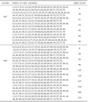
We do similar experiments on the 837- and 838-round Trivium. We find several useful cubes, and we list a part of them in Table 6 in Appendix 2. Among these useful cubes, we recover the exact superpolies of those with fewest tight terms2. For each recovered
superpolypI, we figure out the corresponding setGI and estimate the size of WKI with
220random keys. Furthermore, to recover more key variables, we calculate the conditional
probability P r(g= 1|pI = 1)for eachg∈Ω, and so we could obtain a set
P GI ={g|g∈Ω,P r(g= 1|pI = 1)∈(0,0.25]∪[0.75,1)}.
When pI = 1, we have that g = 1 holds with a probability of P r(g = 1|pI = 1) for
g ∈P GI. Namely, with the setP GI, we could obtain several probabilistic equations on key variables under weak keys. We summarise our results in Table41.
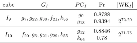
Table 4: Superpolies of 837- and 838- round Trivium
cube GI P GI Pr |WKI|
I9 g7, g22, g30, f21, k56
g0 0.8788
272.20
g13 0.9394
I10 f20, g6, g21, g29, k55 g12 0.8846 271.75 k64 0.78
As a result, for the 837-round Trivium, we could obtain5deterministic and 2 proba-bilistic equations on about272.2weak keys with a complexity of237(|I9|= 37). Similarly,
in the case of the 838-round Trivium, we could obtain5deterministic and 2 probabilistic equations on about 271.75weak keys with a complexity of237 (|I10|= 37).
Interestingly, I10 is the same as the cube proposed by Liu in [16]. Recall that Liu tested 100 random keys for the superpoly of this cube, the values are always0. However, after obtaining the ANF of pI10 with our method, we know that pI10 is not 0-constant.
It indicates that the output of the 838-round Trivium achieves the maximum degree 37
over this subset of IV variables, and so the degree given by Liu for this cube is tight. In Table5, we list several keys under which the values of these two superpolies are1’s, where
key=k7||k6· · · ||k0||k15||k14· · · ||k8|| · · · ||k79||k78|| · · · ||k72.
Table 5: The found secret keys
cube key cube key
I9
0x4fe7af8e2e5e727b31f9
I10
0xffffdfff0f7ff53ff8ff 0x4fe7af8e2e5e737b31f1 0xffffdfff0f7fc53ff8ff 0x4ee7af862e5e727b31f9 0xfbcbd7dfd4bfbdbd5cfc 0x4ee7af8c2e5e727b31f9 0xfbcbd7dfd4bfbdbd3cfc 0x4ee7af862e5e737b31f1 0xfbcbd75fd5afbdbd7cfc
4.3
Discussions
4.3.1 Extra Benefits of Our Method
In our experiments, we find several cubes whose superpolies become 0, i.e., zero-sum
distinguishers, because all the terms are vanished by the xor operations. Such zero-sum
1The details ofI
1, I2,· · ·, I10could be found in Table7in Appendix 1.
2For the detailed ANFs of these found superpolies, please refer to