Liquid Sloshing in Containers:
its Utilisation and Control
Jeremy Graeme Anderson
A thesis submitted to Victoria University of Technology for the Doctor of Philosophy Degree (Mechanical Engineering)
I LIBRARY ^ i
ACKNOWLEDGMENTS
I would like to thank the supervisors of this thesis. Associate Professor Ozden Turan
and Dr. Eren Semercigil. I thank them for their advice, encouragement and
fi-iendship. 1 learnt a great deal fi-om them.
During my candidature I was a recipient of an Australian Postgraduate Award. The
financial support of this scholarship was greatly appreciated. 1 was also given the
opportunity to teach in the Department of Mechanical Engineering and then in the
School of the Built Environment. 1 would like to thank Victoria University of
Technology for this financial help and teaching experience. To the staff and other
postgraduate students, it was a pleasure to work with such a professional team.
FinaUy, to my wife Rachael and my family, I sincerely thank you for your support.
ABSTRACT
Sloshing is the oscillation of a contained liquid. In the first part of this thesis, the
interaction between liquid sloshing and a mechanical oscillator has been exploited to
control resonant vibrations of the oscillator. A deep-liquid-level sloshing absorber is
presented as a practical alternative to the damped tuned absorber. In addition, a
numerical simulation procedure is introduced as a computer aided design tool.
In many practical appHcations, it is necessary to suppress liquid sloshing. Such
applications include the transportation of liquid cargo, sloshing in fliel tanks of
aircraft and spacecraft and earthquake induced sloshing in liquid storage tanks.
Hence, the objective of the rest of the thesis is to control sloshing. Baffles
cantilevered fi-om the sides of tanks have shown effective sloshing control, provided
that the volume of liquid remains approximately constant. Alternatively, a simple
floating control device consisting of two plates in a dumb-bell arrangement has shown
effective control at varying liquid levels.
In some practical applications, the addition of such devices may not be possible due to
geometric constraints. For such cases, the interaction between liquid sloshing and
flexible container walls may be exploited to control liquid sloshing. The advantages
of using a flexible container are twofold. Firstly, liquid sloshing is reduced.
Secondly, if flexibihty of the container is achieved by reducing the wall thickness, a
TABLE OF CONTENTS
Page
ACKNOWLEDGMENTS ii
ABSTRACT iii LIST OF TABLES vi
LIST OF FIGURES vii
Chapter 1
INTRODUCTION 1 Chapter 2
A STANDING-WAVE TYPE SLOSHING ABSORBER TO CONTROL TRANSIENT OSCILLATIONS
2.1. INTRODUCTION 5 2.1.1. Tuned Absorber 6 2.1.2. Sloshing Absorber 7 2.1.3. Use of Liquid Sloshing for Structural Control 9
2.2. RESPONSE OF TUNED VIBRATION ABSORBER 11
2.3. SLOSHING ABSORBER 15 2.3.1. Experiments 16 2.3.2. Numerical Model 20
2.3.3. Results 23 2.4. ON SCALING AND PRACTICAL APPLICATION 34
2.5. AN IMPROVED SLOSHING ABSORBER 39
2.5.1. Numerical Predictions 40
2.6. CONCLUSIONS 53
Chapter 3
CONTROL OF LIQUID SLOSHING USING RIGID CANTILEVER BAFFLES AND FLOATING DEVICES
3.1. INTRODUCTION 56 3.2. EXPERIMENTAL PROCEDURE 60
3.3. CONTROL OF SLOSHING WITH CANTILEVER BAFFLES 65
3.3.1. Results for Cantilever Baffles 66 3.4. CONTROL OF SLOSHING WITH FLOATING DUMB-BELLS 74
3.4.1. Results for Dumb-Bell Controllers 75
3.5. CONCLUSIONS 81
Chapter 4
USING CONTAINER FLEXIBILITY AS A TUNED ABSORBER TO CONTROL LIQUID SLOSHING
4.1. INTRODUCTION 83 4.2. VALIDATION OF THE NUMERICAL MODEL 86
TABLE OF CONTENTS
Page
4.2.2. Numerical Model 89
4.2.3. Results 95
4.3. SLOSHING CONTROL 103 4.3.1. Sinusoidal Excitation 104
4.3.1.1. Tuning 104 4.3.1.2. Results 106 4.3.2. Random Excitation 134
4.4. CONCLUSIONS 146
Chapter 5
CONCLUSIONS 147 REFERENCES 150 Appendix 1
CFX4.1 FILES FOR THE SLOSHING ABSORBER IN CHAPTER TWO 158 Appendix 2
DERIVATION OF THEORETICAL FUNDAMENTAL SLOSHING 176 FREQUENCY
Appendix 3
LIST OF TABLES
Page
Table 2.1. System parameters. In each column, experimental / 17
computational values are given when they differ, fn and ^q represent the
fundamental frequency and the equivalent viscous damping ratio.
Table 2.2. Cell size of each region of the non-uniform grid in Figure 2.6. 23
Table 2.3. System parameters of model (m) and prototype (p) absorber- 39 structure systems.
Table 4.1. Predicted sloshing wave ampHtude in a rigid container for 91 different grid sizes.
Table 4.2. Predicted 1^, 2"** and 3^^^ natural fi-equencies of the container 91 without liquid for different grid sizes.
Table 4.3. Natural fi-equencies of the 1^ and 3'^'^ mode shapes for a container 106 with a wall thickness of 1.5 mm and without liquid.
LIST OF FIGURES
Page
Figure 2.1. A tuned absorber and the structure to be controlled. 6
Figure 2.2. The proposed sloshing absorber on the structure to be controlled: 8 (a) a sloshing absorber without baffles and (b) with a pair of cantilever
baffles.
Figure 2.3. Displacement ( ) and force ( ) histories of the tuned 14 absorber for (a) ^2=0, (b) ^2=0.025, (c) ^2=0.19 and (d), ^2=1.24, respectively.
Figure 2.4. An isometric view of the sloshing absorber filled with water to a 17 depth of 100 mm.
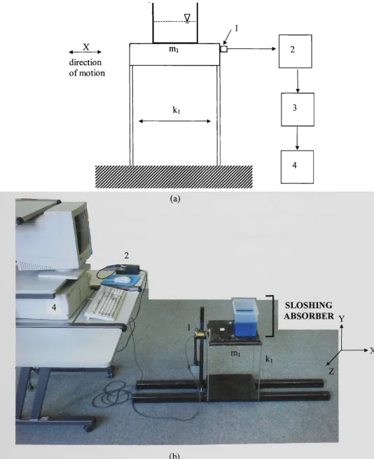
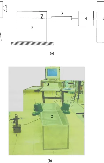
Figure 2.5. (a) Schematic diagram and (b) photograph of the experimental 19 setup.
1. Keyence, LB-12 laser displacement transducer, 2. Keyence LB-72 amplifier and DC power supply,
3. Data Acquisition Analog to Digital conversion board (DT707T), 4. Personal Computer.
Figure 2.6. Numerical grid of the sloshing absorber showing 10 mm long 22 cantilevered baffles located on the static liquid surface.
Figure 2.7. Displacement and force histories of the sloshing absorber, 27 (a) without baffles, (b), (c) and (d) with 10 mm baffles, 5 mm above, 5 mm
below and on the static liquid surface, respectively.
( ) predicted displacement; ( ) experimental displacement; ( ) predicted sloshing force.
Figure 2.8. Non-dimensional sloshing amplitude plotted against baffle 29 position.
Figure 2.9. Force - displacement phase plots of the same cases as in 31 Figure 2.3.
Figure 2.10. Force - displacement phase plots of the same cases as in 31 Figure 2.7.
Figure 2.11. %Energy of the structure plotted against non-dimensional time 33 for the same cases as in Figure 2.9.
Figure 2.12. %Energy of the structure plotted against non-dimensional time 33 for the same cases as in Figure 2.10.
LIST OF FIGURES
Page
Figure 2.14. Displacement ( ) and force ( ) histories of the sloshing 43 absorber, (a) without baffles, (b) with two baffles 10 mm long submerged
5 mm below the static liquid surface, (c) with two baffles 15 mm long submerged 10 mm below the static liquid surface and (d) with one baffle
15 mm long submerged 10 mm below the static liquid surface.
Figure 2.15. Velocity vector plots for a sloshing absorber with no baffles. 46
Figure 2.16. Velocity vector plots for a sloshing absorber with two 10 mm 48 baffles submerged 5 mm below the static Uquid surface.
Figure 2.17. Velocity vector plots for a sloshing absorber with two 15 mm 50 baffles submerged 10 mm below the static liquid surface.
Figure 2.18. Velocity vector plots for a sloshing absorber with one 15 mm 52 baffle submerged 10 mm below the static liquid surface.
Figure 3.1. The horizontal cylindrical container. 60
Figure 3.2. Controllers used in (a) the vertical and (b) the horizontal 63 containers.
Figure 3.3. Showing (a) the schematic diagram and (b) photograph of the 64 experimental setup with a rectangular container on the shaking table.
1. Gearing and Watson SSI00 signal generator and amplifier, 2. Gearing and Watson Type GWV46 electromagnetic shaker, 3. shaking table (buih in house), 4. rectangular container. The liquid fi-ee surface shape, shown in (a), represents uncontrolled sloshing at the fundamental mode.
Figure 3.4. Uncontrolled numerical grid with experimental ( ) and 67 numerical ( ) surface shapes.
Figure 3.5. Controlled numerical grid with experimental ( ) and 68 numerical ( ) surface shapes for 10 mm baffles located at 10 mm above
the static liquid surface.
Figure 3.6. Controlled sloshing wave shapes from experiments ( ) and 69 numerical predictions ( ), using 10 mm baffles located on the static
liquid surface.
Figure 3.7. Variation of the experimental ( • ) and numerical (•) non- 71 dimensional sloshing amplitude with non-dimensional height for 10 mm
LIST OF FIGURES
Page
Figure 3.8. Variation of the non-dimensional sloshing ampUtude with non- 73 dimensional baffle length. Each line corresponds to a peak-to-peak excitation
amplitude of 1 mm (A), 2.5 mm ( • ) and 5 mm ( • ) . Experimental data ( x ) is given only for an excitation amplitude of 2 ± 1 mm.
Figure 3.9. Showing the equilibrium positions of the dumb-bells when the 75 bottom plate is (a) floating on the surface and (b) submerged in liquid.
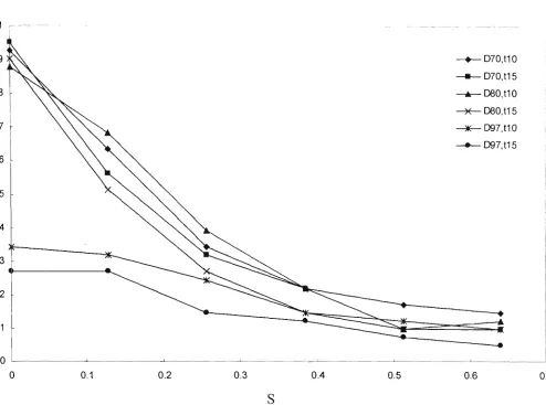
77 Figure 3.10. Variation of non-dunensional sloshing amplitude, A^/AQ, with non-dimensional separation distance, S, for the vertical container. Each symbol corresponds to a set of plates with an outer diameter, D, and plate thickness, t, in mm.
Figure 3.11. Effect of mass ratio on the sloshing wave for non-dimensional 78 separation of the dumb-bell plates (S), of 0, 0.26 and 0.65.
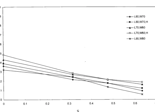
Figure 3.12. Variation of non-dimensional sloshing amplitude, A^./AQ, with 80
non-dimensional separation distance, S, for the horizontal container. Each symbol corresponds to a set of rectangular plates with a length L, and width W, in mm. H denotes hollow plates with a constant 20 mm thickness.
Figure 4.1. Isometric view of the tank with added mass configuration used in 87 the experiment.
Figure 4.2. (a) Schematic view and (b) photograph of the experimental setup. 88 1. video camera, 2. tank, 3. contact displacement transducer (built in house),
4. analogue to digital conversion board (DT707T), 5. Personal computer (Pentium 200MHz).
Figure 4.3. Showing (a) container dimensions and initial conditions and (b) 90 the end view of the container with the shape of the fimdamental sloshing wave
for a rigid container. A and B are the points where displacement histories are observed.
Figure 4.4. Isometric view of the grid used for the container. The cell size is 92 50 mm X 50 mm.
Figure 4.5. Isometric view of the grid used for the liquid. The cell size is 92 50 mm X 50 mm x 50 mm.
Figure 4.6. Mode shapes of oscillation for a container with 1.5 mm thick 94 walls, no added mass and no liquid (a), (b) and (c) 1^ , 2"** and 3"^ mode
LIST OF FIGURES
Page
Figure 4.7. Displacement histories for the wall of the container, 97 (a) experimental displacement, (b) predicted displacement when the liquid is
inviscid and (c) predicted displacement when the liquid has damping.
Figure 4.8. Displacement histories for the liquid, 101 (a) experimental displacement, (b) predicted displacement when the liquid is
inviscid and (c) predicted displacement when the liquid has damping.
Figure 4.9. Displacement histories of the liquid ( ) and container walls 112 ( ) for; (a) rigid wall container, and (b), (c), (d), (e) and (f) a flexible
container with wall thickness of 1.5 mm and added mass of 0 kg, 52.8 kg, 105.6 kg, 165 kg and 198 kg, respectively. The container has 1% damping and the liquid is undamped.
Figure 4.10. Predicted sloshing amplitude for the same cases as shown in 114 Figure 4.9. (a) rigid wall container, (b), (c), (d), (e) and (f) a flexible container
with wall thickness of 1.5 mm and added mass of 0 kg, 52.8 kg, 105.6 kg, 165 kg and 198 kg, respectively. The container has 1% damping and the liquid is undamped.
Figure 4.11. Displacement histories of the liquid ( ) and container walls 118 ( ) for; (a) rigid wall container, (b), (c), (d), (e) and (f) a flexible
container with wall thickness of 1.5 mm and added mass of 0 kg, 52.8 kg, 105.6 kg, 165 kg and 198 kg, respectively. The container has 1% damping and the liquid is damped.
Figure 4.12. Predicted sloshing amplitude for the same cases as shown in 120 Figure 4.11. (a) rigid wall container, (b), (c), (d), (e) and (f) a flexible
container with wall thickness of 1.5 mm and added mass of 0 kg, 52.8 kg, 105.6 kg, 165 kg and 198 kg, respectively. The container has 1% damping and the liquid is damped.
Figure 4.13. Displacement histories of the liquid ( ) and container walls 124 ( ) for; (a), (b), (c), and (d) 0%, 1%, 2% and 5% structural damping. The
wall thickness is 1.5 mm. The added mass is 165 kg and the liquid is undamped.
Figure 4.14. Predicted sloshing amplitude for the same cases as shown in 126 Figure 4.13. The container walls are 1.5 mm thick, the total added mass is
165 kg and the critical damping ratio for the container without liquid is (a) 0%, (b) 1%, (c) 2%, and (d) 5%.
Figure 4.15. Displacement histories of the Uquid ( ) and container walls 129 ( ) for 1 mm wall thickness, 1% Structural damping and 39.6 kg added
LIST OF FIGURES
Page
Figure 4.16. Predicted sloshing amplitude for the same cases as shown in 130 Figure 4.15, 1 mm container waU thickness, a total added mass of 39.6 kg,
(a) no liquid damping and (b) the Uquid is damped.
Figure 4.17. Grid used for the container showing added mass in the middle of 130 the longest walls of the container.
Figure 4.18. Displacement histories of the Uquid ( ) and container waUs 132 ( ) for 1 mm container waU thickness, 1% structural damping and 12 kg
added mass. The Uquid is undamped.
Figure 4.19. Predicted sloshing amplitude for the sanie case as shown in 133 Figure 4.18. 1 mm container wall thickness, 1% structural damping and 12 kg
added mass. The Uquid is undamped.
Figure 4.20. Random excitation given to the base of the container. 135
Figure 4.21. (a) Fourier spectrum and (b) probabiUty distribution for the 136 excitation history in Figure 4.20.
Figure 4.22. Displacement histories of the liquid ( ) and container walls 138 ( ) for random excitation; (a) rigid wall container, and flexible container
with (b) 1.5 mm waU thickness and 165 kg mass added and (c) 1.0 mm wall thickness and 12 kg mass added. Structural damping is 1% and the Uquid is undamped.
Figure 4.23. (a) Sloshing ampUtude, (b) Fourier spectrum and (c) probability 140 distribution for sloshing in a rigid waU container.
Figure 4.24. (a) Sloshing ampUtude, (b) Fourier spectrum and (c) probability 142 distribution for sloshing in a container with 1.5 mm waU thickness.
Chapter 1 INTRODUCTION
The term sloshing generally refers to relatively low fi-equency but large ampUtude
osciUations of a Uquid in a container. The investigations in this thesis are divided into
three separate areas. Firstly, Uquid sloshing has been utilised for the purposes of
controUing structural vibrations. Secondly, the focus has been to control Uquid
sloshing with simple, passive controUers that can be added to existing containers.
Thirdly, the use of container flexibiUty has been examined as a means to control
Uquid sloshing. The general objective is to contribute to the understanding of
sloshing motion in engineering appUcations. To present the specific objectives of this
thesis, a brief description of the content of each chapter is given next. Each chapter is
self-contained, starting with its own introduction and Uterature review.
Liquid sloshing has been utiUsed in the Uterature in Tuned Liquid Dampers (TLD), to
suppress wind induced vibrations of taU structures in a number of appUcations. A
TLD is a passive control device that can suppress structural vibrations using Uquid
motion. There are a number of advantages to using this device, such as low cost of
manufacture and instaUation and low maintenance. No weight penalty to the structure
exists when the design of the damper is incorporated with a storage tank for water
supply. However, existing storage tanks typicaUy have deep Uquid levels that induce
standing sloshing waves. Prior to this thesis, standing sloshing waves had been
shown to have inherently poor energy dissipation characteristics. It is this
phenomenon that is the focus of Chapter 2. In Chapter 2, a deep Uquid sloshing
achieved by strategicaUy placing baffles in the container. The proposed modifications
are simple, inexpensive and can easily be added to many types of storage containers in
practical appUcations. Hence, the significance of the new work presented in Chapter
2 is in its showing that deep Uquid sloshing absorbers can be modified to effectively
control structural osciUations. Previously, such sloshing absorbers were typicaUy
restricted to shaUow Uquid depths only.
The detrimental effects of Uquid sloshing are experienced in areas such as
transportation of Uquid cargo, earthquake induced sloshing in Uquid storage tanks and
the fiiel tanks of aircraft. If not controUed effectively, sloshing may spoU sensitive
items, such as suspension type food, wine and chemical Uquids during transportation.
More importantly, Uquid sloshing can cause loss of dynamic stabUity and
manoeuvrabiUty of the transportation vehicle. In earthquake prone parts of the world,
Uquid sloshing due to ground motion can cause spiUage and may lead to structural
faUure. Therefore, it is important to control sloshing to prevent loss of life and
property. Although there has been wide interest in the modelling of Uquid sloshing,
only few attempted to model the control of Uquid sloshing. In Chapter 3, experiments
and numerical predictions are presented to show that cantilever baffles extending fi-om
the waUs of rigid tanks can provide effective control of Uquid sloshing. One of the
significant contributions in Chapter 3 is that the control action of different sized
cantilever baffles is presented in a non-dimensional form to be used for design
purposes.
Cantilever baffles may not be suitable for aU practical appUcations as their
For cases where the Uquid volume in the container changes, there may be a significant
deterioration of the control action of fixed baffles. In such cases, simple floating
devices may prove successful. Chapter 3 also focuses on an experimental
investigation of a floating device, named a dumb-beU controUer, to suppress Uquid
sloshing when the Uquid level is expected to change over time. Due to the floating
nature of dumb-beU controUers, it is shown that effective sloshing control may be
maintained even when the volume of Uquid in the tank is varied, and this is another
significant contribution in Chapter 3. It is clear that the specifications of practical
problems involving the suppression of Uquid sloshing, wiU ultimately govern the type
of control technique employed.
The addition of passive control devices to control Uquid sloshing may not be possible
in aU appUcations due to structural constraints. Therefore, in Chapter 4, numerical
predictions and experimental observations are given for sloshing control using the
flexibiUty of the container. OsciUations of the container are induced intentionaUy by
tuning the structural natural fi-equencies to that of Uquid sloshing. Such tuned cases
suggest effective control of the Uquid. Hence, the work in Chapter 4 may provide
quite significant benefits in appUcations involving the transportation of Uquid cargo.
Ultimately, the containers used to transport Uquid cargo may act as sloshing
controUers. In addition, if the container waUs are made flexible by reducing the waU
thickness, then significant reductions may be made to the mass of the container. The
significance of Chapter 4 is in presenting this novel concept of exploiting container
In Chapter 5, the conclusions of the thesis are summarised. In addition, three
appendices are included in this thesis. The predictions in Chapter 2 for a sloshing
absorber were done using a commerciaUy avaUable computational fluid dynamics
code, CFX4.1. The two files written in the CFX environment to model the sloshing
absorber are in Appendix 1. Throughout the thesis, the theoretical sloshing fi-equency
is determined and compared with predictions or experiments. The derivation of the
theoretical sloshing fi-equency fi-om MUne-Thomson (1968) is included in Appendix
2, for completeness. As a starting point to modelling dumb-beU type controUers,
some initial numerical predictions are given in Appendix 3 to determine the control
Chapter 2
A STANDING-WAVE TYPE SLOSHING ABSORBER TO CONTROL TRANSIENT OSCILLATIONS^
2.1. INTRODUCTION
The problem of interest in this chapter is the control of excessive vibrations of a
mechanical osciUator in response to an initial displacement. Tuned vibration
absorbers are fi-equently used for this purpose, and if damping is included in the tuned
absorber, the control action is quite effective. The problem, however, is that inclusion
of an energy dissipation element necessitates frequent maintenance in practice. In this
chapter, a deep Uquid sloshing absorber is presented as a practical alternative to the
damped tuned absorber. In addition, a numerical simulation procedure is introduced as
a computer aided design tool.
In contrast to a tuned absorber, a sloshing absorber accompUshes energy dissipation
through sloshing. Therefore, it may be virtuaUy maintenance free. Also, for practical
appUcations, this type of absorber can be an advantage where existing water storage
tanks can be modified to control vibrations of the supporting structure. Numerical
simulations and experimental observations are presented in this chapter to compare
the performances of a sloshing absorber and a conventional tuned absorber. The
scaling parameters of Uquid sloshing in containers are shown to be appUcable to a
system consisting of a sloshing absorber and the structure to be controUed. In
addition, numerical predictions of the velocity field and Uquid free surface shape in a
sloshing absorber are exploited to determine the optimum sloshing absorber
configuration. The tuned absorber and sloshing absorber are described next in detail.
2.1.1. Tuned Absorber
A tuned absorber, in its standard form, is a mechanical oscUlator whose resonant
frequency is tuned at a critical frequency of the structure to be controUed.
Comprehensive treatment of this classical subject may be found in standard textbooks
such as in Hunt (1979) and in Snowdon (1968). Figure 2.1. schematicaUy iUustrates
such a system. The primary system with mass mi, damping ci and stiffiiess ki
represents the structure to be controUed, whereas the auxUiary oscUlator with m2, C2
and k2 is the tuned absorber. Tuning is usuaUy accomplished by designing the natural
frequency of the absorber to be the same as that of the structure to be controUed: (ki /
mi)^^^ = (k2 / m2)^''^. Some sUght deviations from this basic relationship may occur
when using significant values of C2.
STRUCTURE TO BE CONTROLLED
TUNED ABSORBER
With an undamped tuned absorber, control may be very effective when the structure
to be controUed is excited harmonicaUy at the tuning frequency. However, this
effectiveness deteriorates drasticaUy in the case of transient disturbances. In transient
cases, the osciUatory energy may be transferred readUy to the absorber due to strong
interaction. This energy returns to the structure resulting in a poor control action,
unless some means of energy dissipation is provided in the absorber. A damper, C2,
may be included in the absorber to improve performance. Optimum values of
damping are derived in Snowdon (1968), and the response of a tuned vibration
absorber is discussed in detaU here in Section 2.2. Inclusion of a damper, however,
presents problems of frequent maintenance and reduces the practical value of the
controUer. A sloshing absorber may be a simple alternative to the conventional tuned
absorber to avoid such problems.
2.1.2. Sloshing Absorber
Most of the earUer work in the field of sloshing has been directed to understanding the
physics of the phenomenon for the purposes of suppressing it. The objective in this
study is to intentionaUy induce sloshing of a Uquid in a container which is in turn
attached onto a resonant structure. In such a configuration, fluid forces may be used
to counteract and suppress structural osciUations (Anderson et al. 1998a). The
proposed sloshing absorber is shown in Figure 2.2, when attached on the same
structure as in Figure 2.1. In Figure 2.2(a), the sloshing absorber has no baffles.
Alternatively, Figure 2.2(b) shows a sloshing absorber with a pair of baffles
with baffles is discussed in detaU later in Section 2.3. For now. Figure 2.2 is used to
show that the principle of this particular structural control technique is simUar to that
of a classical tuned vibration absorber (Anderson et al. 1998b). However, a distinct
potential advantage of the proposed approach is that existing Uquid storage tanks may
be employed for structural control purposes. For cases where the sloshing controUer
is an added component to reduce structural osciUations, its inherent characteristic of
requiring virtuaUy no maintenance is a significant practical advantage.
SLOSHING ABSORBER
Baffle
(b)
2.1.3. Use of Liquid Sloshing for Structural Control
The concept of using sloshing forces for structural control has been suggested earUer.
FujU et al. (1990) reported using Uquid motion in a circular container to reduce
wind-induced oscillations at Nagasaki Airport Tower and Yokohama Marine Tower to
about half of the uncontroUed values. Abe et al. (1996) reported effective control of
structural vibrations using a U-tube with a variable orifice passage. Modi and Welt
(1984) pioneered research on Nutation Dampers and their appUcations in taU
structures. Seto and Modi (1997) also presented work to use fluid-structure interaction
to control wind induced instabiUties.
In sloshing controUers, plain water, which has poor energy dissipation characteristics,
is usuaUy used as the working fluid. In order to improve energy dissipation, Kaneko
and Yoshida (1994) suggested employing a net to obstruct the flow of Uquid during
sloshing, and reported optimum levels of obstruction for best structural control.
Wamitchai and Pinkaew (1998) predicted the effect of flow damping devices such as
vertical poles, blocks and nets on sloshing in rectangular tanks for the purpose of
controUing structural osciUations. In their formulation, the Uquid was assumed to be
inviscid, incompressible and irrotational. Surface tension effects were neglected.
ShaUow Uquid levels in a container are Ukely to induce traveUing sloshing waves with
desirable energy dissipation. For this reason, earUer work invariably dealt with
shaUow Uquid levels in the tuned sloshing absorbers. Even in the work of Kaneko and
water depth is approximately equal to 35% of the length of the container. Such a
smaU depth may be quite Umiting for some geometries such as Uquid storage tanks in
taU structures. This particular point is addressed in this study with water depth of the
absorber comparable to the length of the container.
Deep Uquid levels cause a standing sloshing wave at the fundamental mode. Without
additional measures, the suppression effect of a standing sloshing wave is quite
limited. For such cases, the oscUlatory energy of the structure could be easUy
transferred to the sloshing Uquid, if there is a strong interaction. A strong interaction
is assured when the sloshing frequency is close to the natural frequency of the
structure. However, if there is no dissipative mechanism in the sloshing absorber, this
transferred energy in the Uquid may travel back to the structure to excite it quite
easUy. OscUlation of energy between the structure and the Uquid, produces a beating
envelope of osciUations of the structure. Such a beat drasticaUy reduces the control
effect, which is discussed in more detaU later in this chapter (Kaneko and Yoshida,
1994, Anderson et al. 1998b).
To improve the performance of a standing wave sloshing absorber, fixed plate baffles
are employed in the Uquid container, as shown in Figure 2.2(b). SimUar baffles were
mvestigated earUer by Muto et al. (1988) where the purpose was to suppress Uquid
sloshing when the Uquid container was excited by external means. In Chapter 3, the
effectiveness of baffle plates to suppress sloshing is demonstrated. In contrast, in
Chapter 2, baffle plates are used to modify the energy dissipation characteristics of a
Next, the response of a tuned vibration absorber is presented in Section 2.2, foUowed
by a detaUed experimental and numerical treatment of the response of sloshing
absorbers with two baffle plates in Section 2.3. In this section, the tuned absorber is
also compared with a sloshing absorber. Practical appUcations and scaUng of sloshing
absorbers are given in Section 2.4. An optimum sloshing absorber, which has only
one baffle, is presented m Section 2.5.
2.2. RESPONSE OF TUNED VIBRATION ABSORBER
The performance of a conventional tuned absorber is examined in this section. A
tuned absorber and the structure to be controUed are shown in Figure 2.1. The mass
of the structure and mass of the absorber are 28 kg and 2.8 kg, respectively. The
stif&iess of the springs used for the structure and absorber are 5826 N/m and 579 N/m
respectively. The structure to be controUed is undamped, Ci = 0. The system
parameters are summarised in Table 2.1.
The structure was given an initial displacement of 1.3 mm, and then the free vibration
response of the system was determined. As shown in detaU in Section 4.3.2, the
response of a structure for a transient disturbance is a good indication of that for
random excitation such as an earthquake. The reason for this behaviour, of course, is
that random excitation may be envisaged as being made up of a series of transient
disturbances in time. For this reason, transient system response has been used in this
chapter in assessing the effectiveness of a tuned vibration absorber, as weU as those of
The solution of the equations of motion of the system shown in Figure 2.1 was
obtained by numericaUy integrating the coupled system of two differential equations
of motion, one for each mass. A standard fourth order Runge-Kutta procedure was
foUowed. The time step was taken to be smaUer than l/40th of the shortest expected
period of osciUations. Details of this procedvire can be found in standard textbooks
such as Rao (1990).
Histories of the displacement of mi ( ) and the control force ( ) of the tuned
absorber on mi, are shown in Figure 2.3. The horizontal axis represents
non-dimensional time, t / To, where To is the natural period of the structure to be controUed
alone. The control force is comprised of the spring force, k2(X2-Xi), and the damper
force C2(X2-Xi), of the tuned absorber, where Xi and Xi and X2 and X2 are the
displacement and velocities of the masses mi and m2, respectively . In Figure 2.3(a),
the absorber is undamped, whereas in Figures 2.3(b) to 2.3(d), the value of critical
damping ratio of the absorber, ^2, is 0.025, 0.19 and 1.24. Here, the critical damping
Q
ratio of the absorber, is defined as, ^2 = ^
2 7 m ^
In Figure 2.3(a), for the undamped tuned absorber, the oscUlatory energy periodicaUy
travels back and forth between the structure to be controUed and the absorber. Due to
this strong interaction, which is the result of tuning the absorber to the natural
frequency of the structure, an initial displacement of 1.3 mm rapidly decays to very
smaU values around 1.8 periods. At this instant, the absorber osciUates quite violently
as indicated by the large control force. Starting from about 2 natural periods, however,
as its initial displacement. This exchange of energy, produces periodic beats of the
envelopes of both displacement and force osciUations. The beat of the two histories
are aUnost perfectly out of phase, indicating where most of the oscUlatory energy is at
a particular time.
In Figure 2.3(b), some Ught damping, ^2 = 0.025, is included in the tuned absorber,
producing a sigruficant difference from the results in Figure 2.3(a). The strong
interaction and the resulting beat are stiU quite clear in Figure 2.3(b). However, the
peak ampUtudes decay graduaUy as a result of energy dissipated due to damping
When ^2 is increased to 0.19 in Figure 2.3(c), the beat disappears completely leaving a
very effective control action. OsciUations virtuaUy stop after 8 periods. In Figure
2.3(d), when ^2 is 1.24, the effective control Ui Figure 2.3(c) deteriorates quite
drasticaUy. Due to havuig too large a resistance between the oscUlator and the
absorber, the absorber is no longer able to osciUate freely with respect to the structure
to be controUed. The Umited relative motion stUl dissipates some energy, resulting in
a slow rate of decay of the osciUation envelope. Any flirther increase in the value of ^2
would worsen the situation, eventuaUy locking m2 on mi and reverting to an
T5 C
m E" E
•a
c a
"E
E
• a c <a E"
E
• a
c E E
A conventional tuned absorber is certainly capable of producing an effective control
action for a value of ^2 around 0.19. This ^2 value is in close agreement with the
optimum value suggested in Snowdon (1968). For such optimaUy damped cases, the
control is so effective that the total energy of the system is dissipated within eight
periods after the Uiitial disturbance. Such tuned absorbers have been used in towers
and bridges (Abu^ et al. 1991). Viscous damping is introduced using hydrauUc
mechanisms which are rather complex and demand continual maintenance. Avoiding
such a need for maintenance should certainly be an advantage in appUcation. The
sloshing absorber discussed ui the next section, is proposed to gaui such an advantage.
2.3. SLOSHING ABSORBER
To examine the response of a structure with a sloshing absorber as shown in
Figure 2.2, first, a Uquid contamer was attached to the osciUator. Then, baffle plates
were added to the container to knprove the control performance. Many different baffle
configurations were simulated with the suggested sloshing absorber. For a sloshing
absorber with two baffles, the baffle length was varied between 2 mm and 30 mm.
The vertical position of the baffles was also varied from 10 mm above the static Uquid
height to 20 mm below the Uquid surface (submerged). The same baffle sizes were
also investigated for a sloshing absorber with one baffle. From the trials with two
baffles, it was clear that with a single baffle, vertical baffle positions ranging from on
the Uquid surface to 20 mm below (submerged) needed to be evaluated.
Baffle configurations were evaluated numericaUy and verified experimentaUy. The
the structure. In Section 2.3.1, the experimental procedure is outUned first. Then, the
numerical model is described in Section 2.3.2. The experimental and numerical
resuUs are compared and the resultmg trends are discussed in Section 2.3.3 for a
sloshing absorber with a pau" of baffles.
2.3.1. Experiments
The sloshing absorber consisted of a rectangular container of 130 mm length by
210 mm width, as shown in Figure 2.4. The container was fiUed with water to a depth
of 100 mm, corresponding to a mass of approxunately 2.8 kg. As indicated in
Figure 2.4, the length of the container used for the sloshing absorber was longer in the
Z direction than in the X direction for two-dimensionaUty. The sloshing absorber was
orientated on the structure to be controUed such that a sloshing wave was induced in
the XY plane. The chosen dimensions of the sloshing absorber resuUed in a virtuaUy
two-dimensional sloshing wave with Uttle motion in the Z direction. The experimental
setup is shown in Figure 2.5.
The structure consisted of a mass of 27.9 kg supported on four 390 mm long mUd
steel colirains of 3.5 mm thickness and 22 mm width. The columns were aUgned so
that they formed an equivalent one-dimensional spring, aUowing the motion of the
structure in the X direction, as shown in Figure 2.5. The ratio of the mass of water in
the container to the mass of the structure was about 10%. The structure exhibited Ught
damping under free vibrations, and it had a natural frequency of 2.6 ± 0.2 Hz. The
fundamental sloshing frequency of the Uquid in the container was 2.3 ± 0.2 Hz.
direction of motion
100 mm
Y
- • X
mm
130 mm
Figure 2.4. An isometric view of the sloshing absorber fiUed with water to a depth of 100 mm.
Table 2.1. System parameters. In each column, experimental / computational values are given when they differ, fn and ^eq represent the fimdamental frequency and the equivalent viscous damping ratio.
Structure
Tuned Absorber
Water
mass (kg)
27.9 / 28
2.8
2.8
Stiffiiess (N/m)
7490 / 6374
585
fn (Hz)
2.6 ±0.2/2.4
2.3
2.3 ± 0.2 / 2.2
^eq
0.004+0 .002
For each test case, the structure was displaced by 1.30 + 0.05 mm before being
released to oscUlate freely. This value was chosen to create a reasonable sloshing
ampUtude m the absorber. The displacement of the structure was tracked with a
Keyence LB-12 laser displacement transducer and then recorded. After determining
the behaviour of the free vibrations of the structure alone, the rectangular container
was secured to the structure. Several series of tests were performed where the Uquid
motion was first left uncontroUed, and then, it was controUed by different cantUevered
The baffles were constructed from 3 mm thick plywood, and the surfaces were sealed
to reduce water absorption. The performance of the sloshing absorber is shown in
Section 2.3.3 for a pair of baffles with cantUevered lengths of 10 mm located at
different distances from the liquid surface. Although many other trials were
performed with two baffle plates, this particular baffle size was found to provide an
optUnal control for the chosen sloshing absorber. Hence, only this set of results is
direction of motion
.2..
mi
k i
(a)
/
SLOSHING ABSORBER y
- • X
(b)
Figure 2.5. (a) Schematic diagram and (b) photograph of the experimental setup. 1. Keyence, LB-12 laser displacement transducer,
2. Keyence LB-72 amplifier and DC power supply,
2.3.2. Numerical Model
A two-dimensional numerical model of the sloshing absorber was created using CFX
Version 4.1 (CFDS-FL0W3D, 1994). For Uquid sloshing, a two-phase model was
adopted because of the presence of a Uquid-gas interface at the free surface. The
Navier-Stokes equations were solved using the Volume of Fluid method (Hirt and
Nichols, 1981). Each phase was assumed to be homogeneous, and a clear defiiution
of the Uquid free surface was obtained by using a surface sharperung algorithm.
Surface tension was not included, and no-sUp condition was imposed at soUd
boundaries. A mass source tolerance of 10*^ kg/s was used to judge convergence uv
single precision. The maximum number of iterations was set to be 50 per time step at
each ceU. This choice was conservative, because convergence was reached in less
than 50 iterations m aU cases.
A viscous model was used, in order to mauitaui the abiUty to simulate a wide range of
cases. As discussed in Section 2.4, an inviscid approach may be sufficient to simulate
the particular sloshing absorber used in this investigation. However, viscous effects
are not negUgible in aU cases of sloshing absorbers in practical appUcations.
Therefore, a general numerical tool capable of including viscous effects is useful.
A two-step solution procedure was foUowed to account for the interaction between the
Uquid and the structure at each time step. First, the structure to be controUed was
given an initial displacement of 1.3 mm. InitiaUy, the control force from the sloshing
absorber was zero, since there was no sloshing of the Uquid. Hence, the solution
connection existed between the structure to be controUed and the sloshing absorber,
the two systems had to experience the same displacement. Therefore, the
displacement of the structure was given to the sloshing absorber next within the same
time step. The pressure distribution on the container waUs was obtained from the
CFX solution of the Uquid motion for the updated displacement. The force of the
sloshing absorber on the structure was obtained by numericaUy integrating the
pressure distribution on the waUs of the absorber. The procedure then continued with
the calculation of the displacement of the structure in response to the control force
from the sloshing absorber.
In order to solve the equation of motion for the structure, a.FORTRAN routine was
developed within the CFX environment usuig the Average Acceleration Method (Rao
1990). The equation of motion for the structure to be controUed, is given in
Equation 2.1, where X,, X, and Xj are the acceleration, velocity and displacement of
the mass. Mi; ki is the stiffiiess and F(t) is the control force of the sloshing absorber,
consisting of the resultant pressure force on the container walls, as a fimction of time.
MiXi + CiXi + k , X i = F ( t ) (2.1)
Grid independence was achieved after evaluatmg a series of mesh refinements. After
testUig grids of 13 x 14, 26 x 28 and 52 x 56 cells, for the sloshing absorber with no
baffles, a grid of 26 x 28 ceUs was determined to be sufficient. For sloshing absorbers
with baffles, a non-uniform grid was needed to provide numerical accuracy in the
region near the baffles. A non-uniform grid of 64 x 70 cells was chosen for the
predicted wave shape. This grid is shown in Figure 2.6. In Figure 2.6, each region of
the grid is given a number. The ceU size in each of these regions is given in
Table 2.2.
For each grid evaluated for the fluid solution, the time step was also varied between
0.00025 s and 0.1 s. A time-step of 0.001 s was determined to be the largest possible
for the numerical results to be independent of the time step. The structural solution
required a time step of 0.01 s, which was 10 times coarser than that of the fluid
solution. The COMMAND and FORTRAN files used to model a sloshing absorber in
the CFX environment are included in Appendix 1.
t:^
2
V
6
^ f f l s s s s s s s s H H H H
llllllll
fiit ^
^==^^== = = = ^ . ^ = ^ ^ = ^= =^ffff||T|T
B B H H B B H H B H ! \ i\
. 1
Table 2.2. CeU size of each region of the non-uniform grid in Figure 2.6.
Region CeU Size mmx mm
1 1 x 5
2 5 x 5
3 1 x 1
4 5 x 0 . 5
5 1 xO.5
6 5 x 1
7 1 x 1
8 1 x 5
9 5 x 5
IiUtial numerical predictions were performed to determine the strongest interaction
between the structure and the Uquid. "Tuning" was observed for a frequency ratio of
0.95. This value represents the ratio of the fundamental sloshing frequency (when the
container is alone), to the structural natural frequency (Uicluding the added Uquid
mass). Although other frequency ratios were tried between 0.8 and 1.2, the
interaction between the sloshing absorber and the structure to be controUed was
strongest for a turung ratio of 0.95. This frequency ratio agrees with those in Hayama
and Iwabuchi (1986) and FujU et al. (1990). The mass of the osciUator, mi, was set to
30.8 kg (consistuig of 28 kg mass of the structure and 2.8 kg mass of the water). The
stiffness of the spring, ki, was 6374 N/m Structural damping was set to zero.
Parameters of the numerical model corresponding to those of the experiments are
listed m Table 2.1.
2.3.3. Results
In Figures 2.7(a) to 2.7(d), the numericaUy predicted ( ) and experimentaUy
observed ( ) displacement histories of the osciUator are given along with the
numerically predicted sloshing force ( ) on the oscUlator for an absorber without
baffles and then with baffles at different positions. Agam, the time is
non-dimensionaUsed with the period of the oscUlator alone. Both experimentaUy and
displacement of 1.3 mm. At the start, the total energy of the combmed system is the
potential energy stored in the spring of the osciUator due to its initial displacement. In
the foUowing paragraphs, numerical predictions are discussed before the comparison
with experiments.
In Figure 2.7(a), after the osciUator is released from 1.3 mm, its ampUtude decays
whUe the ampUtude of the sloshing force increases as the sloshing motion develops.
After approximately 3.5 natural periods, the displacement e5q)eriences its smaUest
ampUtude whereas the sloshing force is at its largest value. This phenomenon
indicates an exchange of energy between the osciUator and the sloshing Uquid. In
contrast to the situation at the start, now most of the energy is with the sloshing Uquid.
This exchange contuiues as the energy is transferred back to the osciUator, around 6.3
periods, and back to the Uquid, around 9 periods, fomung a "beat" envelope of
osciUations.
Strong interaction of the oscUlator with Uquid sloshing is desirable during the initial
stages. This strong interaction assures that the oscUlatory energy is taken away from
the structure to be controUed. However, as mentioned earUer, the Uquid level used in
this study results m a standmg sloshmg wave, which has virtuaUy no effective means
of dissipatmg energy. Hence, the energy in the absorber returns to the oscUlator,
producing a poor control effect. Some additional means of energy dissipation in
Uquid sloshing must be mtroduced to improve control.
In Figures 2.7(b) to 2.7(d) histories of the same three parameters are shown as in
plates cantUevered symmetricaUy from the opposite sides of the container. These
plates are aU 10 mm long and 3 mm thick. In Figure 2.7(b), the baffles are located
5 mm above the static free surface of the Uquid; in Figure 2.7(c) they are submerged
5 mm below the surface, and m Figure 2.7(d) the baffles are on the surface.
In Figure 2.7(b), when the baffle plates are 5 mm above the surface, the response of
the system is identical to that of the no baffle case m Figure 2.7(a), untU the surface
wave reaches a height of 5 mm. This instant is clearly signified around 1.8 periods
where the sloshing force displays some discontinuity. The overaU difference between
Figures 2.7(a) and 2.7(b), however, is quite insignificant. This relative ineffectiveness
could be attributed to minimal interaction between the surface of the Uquid and the
baffle plates smce the Uquid surface is free from contact with the baffles during most
of its cycle.
The best control effect is obtained for the case shown in Figure 2.7(c) when the
baffles are 5 mm below the surface. For this case, the disturbance in the flow is able
to aUow a relatively strong mteraction at the start. After the initial strong interaction,
however, the sloshing Uquid is disturbed enough so that the beat in the envelope of
structural osciUations is much less pronounced. In addition, the structural
displacements are smaUer than 0.25 mm (about one-fifth of the iiutial displacement)
after approximately 5 periods, whereas peak displacements reach up to 1.0 mm for the
case in Figure 2.7(a).
In Figure 2.7(d), when the baffles are on the surface, the beat shown in the preceding
with the osciUator. This in-phase motion between the sloshmg Uquid and the
osciUator, prevents the transfer of energy from the oscUlator to the Uquid as they
move in unison. Therefore, surface baffles modify the sloshing wave too strongly
resulting in a poor control action.
In aU four frames of Figure 2.7, the experimentaUy measured displacement of the
oscillator is also given for comparison purposes. These experimentaUy measured
displacements foUow the same trends as those of the numerical predictions. However,
the experimental frequency of osciUations is about 5% smaUer in Figure 2.7(a) and
5% higher m Figures 2.7(b) to 2.7(d) than the numerical ones. In addition, especiaUy
for the two more effective cases in Figures 2.7(b) and 2.7(c), when the baffles are
5 mm above and below the surface, respectively, the experimentaUy observed control
of the structure is more effective than predicted. This pronounced effectiveness may
be attributed to the dissipation of energy due to the surface roughness of the baffles
and the contakier, surface tension effects and Ught structural damping which are not
included in the numerical model. For the case when the baffles are at the surface in
Figure 2.7(d), the experimentaUy measured displacements have just as ineffective a
control as the numerical predictions, due to the in-phase motion discussed earUer in
the previous paragraph. Even with the differences, the comparisons clearly indicate
that the numerical predictions are able to capture the sigruficant trends in the control
action. The numericaUy predicted structural control may be conservative, assuring
that the control may weU be better in appUcation. Hence, the numerical model is
certainly a useful tool to predict performance and to select the promising
Figure 2.7. Displacement and force histories of the sloshing absorber, (a) without baffles, (b), (c) and (d)
with 10 mm baffles, 5 mm above, 5 mm below and on the static Uquid surface, respectively.
The trends observed in Figure 2.7, where the baffle plates are positioned at different
locations from the surface of the Uquid, may be explained in relation to the
information presented in Figure 2.8. The results in Figure 2.8 correspond to the same
contakier as the one used to generate the results Ui Figure 2.7. In Figure 2.8, what is
presented is the control of Uquid sloshmg and not structural control using Uquid
sloshing. The container is excited sinusoidaUy at the fimdamental sloshing frequency
with a peak-to-peak ampUtude of 2.5 nun. Although a fiiU description of the modified
experimental setup and results for the control of Uquid sloshing wiU be given in
Section 3.2 and Section 3.3, respectively, of Chapter 3, it should be noted here that a
setup simUar to that in Figure 2.5 was used to obtain the results presented in
Figure 2.8. The horizontal axis of Figure 2.8 shows the position of the baffles at
5 mm intervals from 10 mm under the surface (negative values) to 10 mm above the
surface (positive values). The numerical predictions are marked with ( • ) , whereas
( • ) Uidicates the corresponding experimental observation. The vertical axis, A/Ao,
represents the ratio of the ampUtude of the sloshing wave with a pair of baffles, Ac, to
that without baffles, Ao. Hence, any reduction in the sloshing ampUtude is reflected
with a ratio smaUer than 1.0.
Numerical predictions consistently uidicate at least a 75% reduction for aU baffle
locations up to the Uquid surface, indicated by 0 mm position on the horizontal axis.
Then, the reduction effect deteriorates aUnost proportionaUy with the baffle distance
from the free surface. As before, experiments ( • ) show consistently more effective
control than what could be predicted numericaUy ( • ) for aU cases. Similarly, this
difference is attributed to the surface tension and waU roughness effects which were
measurable ampUtude could be observed experimentaUy, resulting in perfect sloshing
control. For this case, the Uquid acted as if it was just an added mass ui the container
movuig m perfect phase with it. For the results presented in Figure 2.7(d), when the
same container was attached as the controUer on the oscUlator, the same overly
suppressed sloshing wave was observed which prevented the transfer of energy from
the osciUator. As resuU of this too effective sloshing control, the sloshing absorber
behaved sunUarly to the overdamped tuned absorber m Figure 2.3(d). Figure 2.8 wUl
be re-visited in Section 3.3 of Chapter 3 in relation to the control of Uquid sloshing.
Ao
0.8 0.6 0.4 0.2
Numerical
Experimental
-10 mm -5imn 0mm 5mm
Baffle position from the liquid free surface
10i
Figure 2.8. Non-dimensional sloshing ampUtude plotted agakist baffle position.
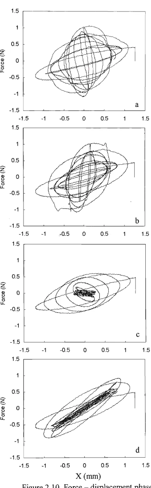
In Figures 2.9 and 2.10, force versus displacement phase plots are given for the tuned
absorber and the sloshing absorber, respectively. The diamond shaped phase pattern
of the undamped tuned absorber in Figure 2.9(a) is also noticeable m that of the
sloshing absorber in Figure 2.10(a). In Figure 2.9(a), the trace of force-displacement
is characterised by a series of elUpses formed either in counter-clockwise or in
clockwise dUections. By changmg thek dkection of rotation, the elUpses cross over
one another creatkig many kitersections, representing a poor control action. For the
fluid. Figure 2.10(b) shows that the performance of the sloshmg absorber with baffles
above the surface is sknUar to that of a Ughtly damped tuned absorber shown ki
Figure 2.9(b). The optimal cases of both absorbers are given m Figures 2.9(c) and
2.10(c). These phase plots have a distkict counter-clockwise pattern that forms a
spkal towards the origin. As indicated by a comparison of Figure 2.10(d) with
Figure 2.9(d), the surface baffles make the sloshing absorber behave Uke an
overdamped tuned absorber. In Figure 2.10(d), smaUer eUiptical areas are enclosed
for each cycle of osciUations than the corresponding optimal case in Figure 2.10(c),
due to the mostly ki-phase trend of the displacement and force. The slope of the
longer axis of the elUpses kidicates the stif&iess of the oscUlator. For the tuned
absorber, the elUpses are concentric with a constant slope. However, for the sloshing
2.5 1.5
i
£ -0.5 -1.5 -2.5 2.5 1.5 0.5 £ -0.5 -1.5 -2.5-2.5 -1.5 -0.5 0.5 1.5 2.5
b
-2.5 -1.5 -0.5 0.5 1.5 2.5
-1.5 -1 -0.5 0.5 1 1.5
-1.5 -1 -0.5 0 0.5 1 1.5
X(mm)
Figure 2.9. Force - displacement phase
1.5 0.5 Q) 0 o " o -0.5 -1
-1.5 a
1.5
1
-0.5
o
L l .
-0.5
-1
-1.5
-1.5 -1 -0.5 0 0.5 1 1.5
b
-1.5 -1 ,ra5 0 0.5 1 1.5
-1.5 -1 -0.5 0 0.5 1 1.5
-1.5 -1 -0.5 0 0.5 1 1.5
X(mm)
Histories of the transient energy of the oscUlator are shown for the same undamped,
Ughtly damped, optimaUy damped and overdamped cases from frame (a) to frame (d)
ki Figures 2.11 and 2.12 for the tuned and the sloshing absorbers, respectively. These
histories are obtakied from the cumulative product of the velocity of the osciUator and
the control force. The product of the control force and osciUator velocity is the
instantaneous power in the osciUator. Summing this power over time consequently
represents energy. Figure 2.11(a) has large fluctuations of energy due to the strong
beat. In Figure 2.11(b), there is some dissipation due to Ught damping. However,
beat kistances are clearly marked as the oscUlatory energy is exchanged between the
structure and the tuned absorber. Figure 2.11(c) corresponds to the optimal dampkig
with a steep slope of decay and no beat. The overdamped tuned absorber results ki
poor mteraction between the structure and the absorber as shown in Figure 2.11(d).
Hence, the energy dissipation rate is smaU.
In Figure 2.12, simUar comments are vaUd for the sloshing absorber as those for the
tuned absorber. In Figure 2.12(a) with no baffles, however, the beat period is
approximately twice as long as ki Figure 2.11(a), and there is some energy loss. In
Figure 2.12(b), the energy dissipation rate is margmaUy enhanced with the beat stUl
clearly apparent when the baffles are 5 mm above the free surface. The most effective
dissipation of energy corresponds to the case in Figure 2.12(c) where the baffle plates
are 5 mm under the surface. In Figure 2.12(d), sloshing wave is suppressed too
effectively with the surface baffles resultkig ki poor energy exchange and poor rate of
energy dissipation. The loss of energy can be attributed to two reasons in the case of
a sloshing absorber. Fkst, it can be due to the occasional phase difference between
the control force and the structure's velocity. Secondly, it can be due to momentum
exchange between the translational and rotational fluid motions over a baffle plate, as
100
0) lU
100
100 100
100
Figure 2.11. %Energy of the structure plotted
0 2 4 6 8 10 12 t/T„
2.4. ON SCALING AND PRACTICAL APPLICATION
In cases where fiiU-scale experiments are expensive or dangerous, scaled experiments
and numerical predictions are needed to determine potentiaUy promiskig solutions.
To this end, scaUng is appUed to the entke absorber-oscUlator system so that the
promiskig resuUs of the sknulations presented earUer can be scaled to systems of any
practical size, without having to perform new sknulations (Anderson et al. 1998c).
LUce many other phenomena kivolvkig Uquids with free surfaces, Uquid sloshmg can
be scaled using Froude, Reynolds, and Euler numbers. Bass et al. (1985) used Froude
and Euler scaling to conduct experiments for Uquid sloshing of 1/30* to 1/50* size of
prototype tanks containing Uquefied natural gas. Muto et al. (1988) also used Froude
scaUng to represent Uquid sloshkig ki a prototype tank with a 1/30* scale model uskig
water as the workkig fluid. The difference between the present work and the earUer
appUcations is that here, there is significant fluid-osciUator mteraction. In addkion,
there is strong interaction between Uquid sloshing and the baffle plates. In this
section, the scaling parameters developed for Uquid sloshing are appUed to a sloshing
absorber coupled to a mechanical osciUator. Froude number is used to scale
displacement and tkne. Reynolds and Euler numbers are used to scale viscosity and
pressure force, respectively.
ScaUng starts by selectkig a geometric scale, a, a=LmfLp where L is the contakier
length, and the subscripts m and p denote the model and the prototype, respectively.
prototype systems. The mass ratio of the Uquid to the osciUator is kept the same for
the model and the prototype. Having selected a, the mass of the Uquid in the scaled
absorber can be calculated by makitaining Pm = Pp where p is the Uquid density. After
determining the dknensions of the prototype absorber, Froude scaling is used for
displacement and tkne scaling. Froude number is the ratio of kiertial to gravity forces
for flows with free surfaces, and it is defined as:
F r = ^ (2.1)
where X and V are the displacement and velocity, respectively, of the coupled
absorber-osciUator system, and g is the gravitational acceleration. For a model wave
scaled to a prototype wave, Froude scaUng (having equal values of the Froude number
for both the model and the prototype) results ki the foUowkig relationships for
displacement, X, and velocky, V:
SinceX = X a, m p
V = V V a . m p
Hence,
T = T Vo^ (2.2) m p
Here, the relationship for T is used to scale the period of structural osciUations as weU
as the period of sloshing m the absorber.
The expression govemkig T can also be obtakied uskig the Strouhal number. Strouhal
number is used for oscUlatkig flows, and it represents a velocity ratio. Here, Strouhal
number is defined as, St = where f is the sloshing frequency, L is the container
length and .^/gL is the characteristic velocity, (Popov et al. 1992). In this
representation, .^/gL is used to denote the characteristic mean fluid velocity, because
the actual mean speed of a standmg sloshing wave is about zero, due to the osciUation
of the wave about the static Uquid position. This form of St is used here for
Uquid-structure interaction due to controUed sloshing for the purpose of structural control.
The period of sloshing can be determined, skice f = —.
Reynolds number. Re, is the ratio of kiertial to viscous forces, and k is used here to
scale viscous effects. For Uquid sloshing, Reynolds number is defined as,
Re=Pt^/iL ^^^^
where [i, p and L are the absolute Uquid viscosity, Uquid density and contakier length
ki the dkection of Uquid sloshing, respectively. Here again, as in Strouhal niunber,
.^gL is the characteristic velocky. If viscous effects are knportant, then Re is kept
3
constant, Rcm = Rcp, by scaUng kkiematic viscosity, v = —,as v„ =a^v . Bass et al.
P
(1985) reported that for sloshkig ki tanks contakung Liquefied Natural Gas, viscous
effects were kisignificant if Re was larger than 10^, and for such cases, viscous
scaling need not be considered. This conclusion is in close agreement with the
observations given by Popov et al. (1993) for Uquid sloshkig ki horizontal cyUndrical
road contakiers. Popov et al. showed that viscosity had no effect for Re ki the range
10^-10^, and the effect was smaU for Re ki the range 10^ - 10^. Therefore, the Uquid
in the model absorber need orUy to have a density sknUar to that of the Uquid ki the
For Re less than 10^ ki the prototype absorber, viscosity wiU have some effect on
Uquid sloshing, and scaUng of viscosky may be knportant.
Euler number, Eu, is the ratio of pressure to inertial forces, and it has been used here
to scale pressure force on the walls of the absorber due to sloshing. Euler number is,
Eu = ^ (2.4) pv2
where P is pressure. Euler number is the same in the model and prototype absorbers.
Therefore, substituting V = V Va from Equation 2.2 gives,
P p
- ^ = a ^ (2.5) P p
P P
Skice pressure is the distributed load per uiut area,
- ^ = a^ (2.6) F
P
for Pm=Pp, where F is the pressure force on the contakier walls, which is the control
force on the osciUator. Uskig this relationship, the force ampUtude for the prototype
system can be determined from that of the model system. To obtain the force history
for the prototype, tkne scaling is also needed, as defined ki Equation 2.2.
As an example, the model used for the analysis presented ki the earUer sections of this
thesis was scaled to a larger prototype system, uskig a=0.026. This geometric scale
value was chosen to give an absorber of 5000 mm length and 8100 mm width,
contakung 158,427 kg of water representkig a water storage tower as the prototype.
To compare the two systems, the displacement and force magnitudes were scaled
uskig Equations 2.2 and 2.6, respectively. Hence, a displacement of 1.3 mm and a
force of 0.4 N for the smaU system corresponded to 50 mm and 22,760 N,
respectively, for the larger system.
The vaUdky of scaling was checked by predicting the response of the prototype
system The results obtakied for the model system were dupUcated identicaUy. These
results were presented in Figure 2.7 earUer. Hence, the suggested scaUng procedure is
usefiil for this highly non-linear system with strong fluid-osciUator and fluid-baffle
plate interactions.
The Reynolds number for the model and prototype cases was 150,000. Therefore,
viscous effects were expected to be insignificant. This pokit was also verified
numericaUy with a case of 10"'' Ns/m^ viscosity and sUp waU conditions. Identical
results to Figure 2.7 were obtakied for this "inviscid" case. Hence, scaling viscosity
through the Reynolds number can be relaxed for the chosen example, smce Re>10^.
The effect of waU surface roughness and flexibiUty have not been taken into account
ki this discussion on scaUng. Therefore, the scaUng procedure outUned here is for
smooth and rigid waU contakiers. Proper representation of waU roughness requkes a
Reynolds number defined with the nomkial roughness height. The viscous effects
associated with waU roughness can be represented with such a Reynolds number
(SchUchtkig, 1979). WaU flexibUity, on the other hand, causes the Uquid sloshing
frequency to be tkne dependent as shown ki Chapter 4, due to vaiykig contakier
Table 2.3. System parameters of model (m) and prototype (p) absorber-structure systems.
Ll (mm) Contakier length (X dkection) L2 (mm) Contakier length (Z dkection) Depth of submerged baffle (mm) Baffle length (mm)
Liquid Depth (mm)
Initial Displacement (mm) Reynolds Number
Liquid Viscosity (Ns/m^) Liquid Density (kg/ m"*)
Fundamental Sloshkig Frequency (Hz) Liquid Mass (kg)
Structural Mass (kg) Spring Stiffness (N/m)
Structural natural frequency (Hz) Tkne Step (sec)
Numerical Model 130 210 5 10 100 1.3 150000 0.001 . 1020 2.2 2.8 28 6374 2.4 0.001 Numerical Prototype 5000 8100 192 384 3800 50 150000 0.24 1020 0.35 158427 1584270 9376283 0.39 0.006
2.5. AN IMPROVED SLOSHING ABSORBER
In this section, a sloshing absorber is re-examined for two reasons. Fkst, an
explanation is suggested for the effectiveness of the baffled standing-wave sloshing
absorber presented previously in this chapter, and in Anderson et al. (1999b and
1999c). Secondly, based on this explanation, a modified sloshing absorber is
described, which has a single baffle, as shown in Figure 2.13.
As indicated at the start of this chapter, the works of FujU et al. (1990), Abe et al.
(1996), Kaneko and Yoshida (1994) and Seto and Modi (1997), dealt with shaUow
Uquid levels ki the sloshing absorbers. At shaUow depths, a travelling sloshing wave
occurs. Travelling sloshkig waves are preferable to standmg waves because of thek
standmg sloshkig waves have been reported earUer (Kaneko and Yoshida, 1994). In
the present kivestigation, deep Uquid levels have been used to kitentionaUy create
standing sloshing waves for use ki practical skuations.
At the fimdamental mode, the standkig sloshing wave ki the absorber is timed to the
natural frequency of the structure to be controUed. As discussed earUer, an optimal
tuning ratio exists. Numerical simulations are given in this section to demonstrate the
performance of an Unproved sloshing absorber ki controUing the excessive transient
vibrations of a resonant structure. As done earUer ki assesskig the effectiveness of a
tuned vibration absorber and double-baffled sloshing absorber, the knproved absorber
with a single baffle is evaluated for a transient disturbance on the structure.
2.5.1. Numerical Predictions
The same numerical procedure reported earUer ki Section 2.3.2 of this chapter is used
here. The system parameters are summarised ki Table 2.1. The sloshing absorbers
evaluated in Section 2.3 have two cantUever baffle plates. One plate is located on
each of the left and right vertical walls of the contakier. The new design
configuration for the sloshing absorber has orUy one baffle plate, and k is shown ki