Optimal Controller Synthesis for Nonlinear Systems

(1)

Optimal Controller Synthesis for Nonlinear Systems

Thesis by

Yoke Peng Leong

In Partial Fulfillment of the Requirements for the degree of

Control and Dynamical Systems

CALIFORNIA INSTITUTE OF TECHNOLOGY Pasadena, California

2018

(2)

(3)

ACKNOWLEDGEMENTS

Graduate school is not always smooth sailing. The beginning and the completion of my thesis would not have happened without these important people in my life. First and foremost, I would like to express my gratitude to my adviser, Prof. Joel Burdick, for his generosity and patience. His guidance is what made this thesis possible. I also appreciate the time he took to provide advices on my professional career beyond research. I would also like to thank my co-adviser, Prof. John Doyle, for his stimulating research discussions and the wealth of interesting research ideas. He opens up my originally narrow view of control to applications beyond traditional engineering. Both of them have provided me the opportunity and freedom to explore, learn, and do many different things in research and beyond during my time at Caltech.

I would also like to thank my thesis committee, Prof. Richard Murray and Prof. Aaron Ames, for their time and advice on improving my thesis. In addition, I want to thank Prof. Richard Murray for being available when I need advices on navigating the academic life and making decisions related to my future career path.

Apart from that, I would like to thank Matanya Horowitz for his guidance in the beginning of my graduate career when I am lost in the ocean of research. This thesis would have been totally different without him. The summer of 2014 at Spain marked the beginning of a productive collaboration with Prof. Pavithra Prabhakar, who introduced me to a fascinating area of research that becomes a part of this thesis. I would like to thank her for hosting me back then, and for her continuous guidance since then.

Life at Caltech would have been so much more mundane without my colleagues and friends in the CMS department, in particular, my classmates, Yorie Nakahira, Ania Baetica, Ioannis Filippidis, and Yuh-Shyang Wang. Stimulating discussions we had in Annenberg have inspired me in many ways in my research. In addition, I would have so much difficulties navigating the world of partial differential equations without my colleague and friend, Albert Chern, who spent hours selflessly answering all my questions related to applied mathematics. Of course, besides research, I appreciate all the great memories we have created and shared on campus and beyond.

(4)

Prof. Todd Murphey. He introduced me to the world of research when I was young and clueless, and convinced me to choose Caltech when I was torn between staying or leaving my alma mater, Northwestern University, for graduate school. His words of advice and his energy and enthusiasm are what keeps me going when times are difficult at Caltech.

(5)

ABSTRACT

Optimal controller synthesis is a challenging problem to solve. However, in many applications such as robotics, nonlinearity is unavoidable. Apart from optimality, correctness of the system behaviors with respect to system specifications such as stability and obstacle avoidance is vital for engineering applications. Many exist-ing techniques consider either the optimality or the correctness of system behavior. Rarely, a tool exists that considers both. Furthermore, most existing optimal con-troller synthesis techniques are not scalable because they either require ad-hoc design or they suffer from the curse of dimensionality.

This thesis aims to close these gaps by proposing optimal controller synthesis tech-niques for two classes of nonlinear systems: linearly solvable nonlinear systems and hybrid nonlinear systems. Linearly solvable systems have associated Hamilton-Jacobi-Bellman (HJB) equations that can be transformed from the original nonlinear partial differential equation (PDE) into a linear PDE through a logarithmic trans-formation. The first part of this thesis presets two methods to synthesize optimal controller for linearly solvable nonlinear systems. The first technique uses a hierar-chy of sums-of-square programs to compute a sequence of suboptimal controllers that have non-increasing suboptimality for first exit and finite horizon problems. This technique is the first systematic approach to provide stability and suboptimal performance guarantees for stochastic nonlinear systems in one framework. The second technique uses the low rank tensor decomposition framework to solve the linear HJB equation for first exit, finite horizon, and infinite horizon problems. This technique scale linearly with dimensions, alleviating the curse of dimensionality and enabling us to solve the linear HJB equation for a quadcopter model that is a twelve-dimensional system on a personal laptop. A new algorithm is proposed for a key step in the controller synthesis algorithm to solve the ill-conditioning issue that arises in the original algorithm. A MATLAB toolbox that implements the algorithms is developed, and the performance of these algorithms is illustrated by a few engineering examples.

(6)

(7)

PUBLISHED CONTENT AND CONTRIBUTIONS

[1] Y. P. Leong and P. Prabhakar, “Abstraction-refinement based optimal control with regular objectives,” arXiv:1504.02838, 2017,

Y.P.L. participated in the conception of the project, derived and analyzed the solution technique, developed the numerical tool, and participated in the writing of the manuscript.

[2] Y. P. Leong and P. Prabhakar, “Optimal control with regular objectives using an abstraction-refinement approach,” in American Controls Conf. (ACC), 2016, pp. 5161–5168. doi:10.1109/ACC.2016.7526478,

Y.P.L. participated in the conception of the project, derived and analyzed the solution technique, developed the numerical tool, and participated in the writing of the manuscript.

[3] Y. P. Leong, M. B. Horowitz, and J. W. Burdick, “Linearly solvable stochastic control lyapunov functions,” SIAM Journal on Control and Optimization, vol. 54, no. 6, pp. 3106–3125, 2016. doi:10.1137/16M105767X,

Y.P.L. participated in the conception of the project, derived and analyzed the solution technique, and participated in the writing of the manuscript. [4] E. Stefansson and Y. P. Leong, “Sequential alternating least squares for

solv-ing high dimensional linear Hamilton-Jacobi-Bellman equation,” in IEEE Int. Conf. on Intelligent Robots and Systems (IROS), 2016, pp. 3757–3764.

doi:10.1109/IROS.2016.7759553,

Y.P.L. participated in the conception of the project, and participated in the writing of the numerical tool and the manuscript.

(8)

Optimal Control Synthesis for Hybrid Systems with

Qualitative and Quantitative Objectives

Chapter 9: Optimal Controller Synthesis for Regular Objectives . . . 125

9.1 Controller Synthesis for Regular Objectives . . . 125

9.2 Controller Synthesis for Hybrid Systems . . . 129

9.3 Implementation . . . 133

9.4 Summary . . . 138

Chapter 10: Optimal Controller Synthesis forω-Regular Objectives . . . 139

(10)

Appendix D: Proofs for Chapter 10 . . . 157

D.1 Proof of Theorem 10.1 . . . 157

D.2 Proof of Theorem 10.2 . . . 158

Chapter 11: Conclusion . . . 163

(11)

LIST OF ILLUSTRATIONS

Number Page

4.1 An example of increased error with non-increasing bound. . . 35 4.2 Desirability function of a 1D system (4.20) using SOS programs. . . 50 4.3 Computational results of a 1D system (4.20) using SOS programs. . . 51 4.4 Desirability function of a 2D system (4.21) using SOS programs. . . 53 4.5 Computational results of a 2D system (4.21) using SOS programs. . . 54 5.1 A simulation of a quadcopter using the controller from Algorithm 2

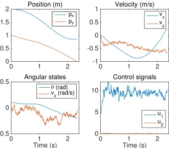
and SeALS (Algorithm 7). . . 64 5.2 State, input, and cost trajectories of a simple pendulum stabilization

using the controller from Algorithm 4 with scaling. . . 68 5.3 State trajectories of a VTOL aircraft using the controller from

Algo-rithm 6. . . 70 5.4 An example of an ill-conditioned matrixM in (3.21) for Example 5.1. 72 5.5 Computational results of using Algorithm 1 on Example 5.1 with and

without sequential solutions. . . 73 5.6 Computational results of using Algorithm 1 on Example 5.1 with and

without boundary condition rescaling. . . 75 5.7 Computational results of implementing sequential computation on

Example 5.1 with and without boundary condition rescaling. . . 76 5.8 Solution and basis functions in each dimension for Example 5.1. . . . 78 5.9 Residual kAF−Gk

q Îd

i=1ni

and normalization constantss_lF for Example 5.1. . . 79 5.10 Simulations of Example 5.1 using the controller from Algorithm 2

and SeALS (Algorithm 7). . . 79 5.11 Comparison of the state trajectories of Example 5.1 using the

con-trollers computed from SOS programs in Chapter 4 and tensor based Algorithm 2 with SeALS (Algorithm 7). . . 80 5.12 Comparison of the control input trajectories of Example 5.1 using the

controllers computed from SOS programs in Chapter 4 and tensor based Algorithm 2 with SeALS (Algorithm 7). . . 81 5.13 Comparison of the cost using the controllers computed from SOS

(12)

A.1 The desirability function and the basis functions in each dimension

and the normalization constantss_lF for Example A.3. 87 A.3 A simulation of Example A.3 using the controller from Algorithm 2

and SeALS (Algorithm 7). . . 87

and normalization constantss_lF for Example A.4. . . 89 A.6 A simulation of Example A.4 using the controller from Algorithm 2

and SeALS (Algorithm 7). . . 90 A.7 A simulation of Example A.5 using the controller from Algorithm 2

and SeALS (Algorithm 7). . . 91 A.8 The control signals for the simulation of Example A.5. . . 91 A.9 Seperation rank of the desirability function for Example A.2

com-puted from Algorithms 3 and 4. . . 93 A.10 Scaling constants of the desirability function for Example A.2

com-puted from Algorithms 3 and 4. . . 93 A.11 Basis functions and desirability function of Example A.2 computed

from Algorithm 3 at timet =0 seconds. . . 94 A.12 Basis functions and desirability function of Example A.2 computed

from Algorithm 3 at timet =2.5 seconds. . . 94 A.13 Basis functions and desirability function of Example A.2 for

Algo-rithms 3 and 4 at the final timet =5 seconds. . . 95 A.14 State, input, and cost trajectories of Example A.2 using the controller

from Algorithm 3. . . 95 A.15 Basis functions and desirability function of Example A.2 computed

from Algorithm 4 at timet =0 seconds. . . 96 A.16 Basis functions and desirability function of Example A.2 computed

from Algorithm 4 at timet =2.5 seconds. . . 97 A.17 State, input, and cost trajectories of Example A.2 using the controller

from Algorithm 4. . . 97 A.18 Convergence of eigenvalue of Example A.1. . . 99 A.19 State, input, and cost trajectories of Example A.1 using the controller

from Algorithm 6. . . 100 A.20 State, input, and cost trajectories of Example A.1 using the controller

(13)

A.21 Convergence of eigenvalue of Example A.2. . . 103 A.22 State, input, and cost trajectories of Example A.2 using the controller

from Algorithm 6. . . 104 A.23 State, input, and cost trajectories of Example A.2 using the controller

from LSOC. . . 105 A.24 Convergence of eigenvalue and error of Example A.4. . . 106 A.25 State and input trajectories of Example A.4 using the controller from

Algorithm 6. . . 107 7.1 An example of a regular property and corresponding paths given by

a winning strategy. . . 117 7.2 An example of a ω-regular property and the corresponding Büchi

automaton. . . 118 9.1 An illustration of a chain strategy and refinement. . . 131 9.2 Automaton that represents the regular objective for the two examples. 134 9.3 Simulated result ofOptCARand LQR for System (9.1). . . 135 9.4 A schematic of a two-tank system. . . 135 9.5 Partitions for the two-tank system. . . 136 9.6 State trajectory and control input generated by the controller from

OptCARfor System (9.2). . . 137

(14)

LIST OF TABLES

Number Page

(15)

ABBREVIATIONS

ALS. Alternating least squares.

CLF/SCLF. Control Lyapunov function/stochastic control Lyapunov function.

CP. CANDECOMP/PARAFAC.

HJB. Hamilton-Jacobi-Bellman.

LQG. Linear quadratic Gaussian regular.

LQR. Linear quadratic regular.

LSOC. Linear stochastic optimal control.

PDE. Partial differential equation.

SeALS. Sequential alternating least squares.

SOS. Sum-of-Squares.

(16)

LIST OF NOTATIONS

Notations commonly used throughout the thesis are listed here. Notations specific to a particular chapter are defined individually in the corresponding chapter.

Sets

Z All integers.

Z+ All positive integers (excluding zero).

N All natural numbers (including zero). R All real numbers.

R+ All nonnegative real numbers.

Rn Alln-dimensional real vectors. Rn×m Alln×mreal matrices.

Function Classes

Given a function classF, with abuse of notation, letF (x)denotes all real functions ofx ∈_Rn_and_{F (}_Ω₎_{denotes all real functions of} _x _∈_Ω _⊆

Rn.

R All real polynomial functions.

Rn×m _{All matrices of size}_n_×_m_{such that}_M

i,j ∈ R ∀i, j.

K All real continuous nondecreasing functionsµ: R+ → R+ such that µ(0)=0, µ(r)> 0 ifr > 0, and µ(r) ≥ µ(r0)ifr > r0.

Ck All realk-differentiable functions f.

Ck,k0 All real functions f such that f is k-differentiable with respect to the first argument and k0-differentiable with respect to the second argument.

L_p All realp-th integrable functions f, where ∫ |f|pdx

1

p < ∞.

SOS All real sum-of-squares polynomials f.

S All real separable functions f :Rn→Rsuch that f(x)=Ír_i₌₁siÎd_j₌₁ f_ji(xj), where f_ji ∈ C∞(xj)andxjis the j-th component ofx.

Sn×m _{All matrices of size}_n_×_m_{such that}_M

i,j ∈ S ∀i,j.

Sequences

[k] An integer sequence from 0,1, . . . ,k.

(17)

{xi}_in₌_m A sequencexm,xm+1, . . . ,xn−1,xn, wheren ≥ m.

{xi}i∈[n] A sequencex0,x1, . . . ,xn−1,xn.

Norms

Let x ∈_Rnbe a vector, M ∈_Rn×nbe a matrix, f ∈ C∞(Ω)be a function onΩ, and Fbe a CP tensor function.

kxk_∞ maxk∈[n]₊|xk|.

kxk₁ Í

k∈[n] |xk|.

kfk_∞ sup_x_∈_Ω|f(x)|if exists.

kMk_F Frobenius normqÍn_i₌₁Ín_j₌₁|Mi j|2_.

kMk_∞ max_i∈[n]₊Ín_j₌₁|Mi j|.

kFk phF,Fi.

Others

Let x ∈ _Rnbe a vector, M ∈ _Rn×nbe a matrix, f ∈ C∞(Ω)be a function onΩ, A

be a set, andFbe a CP tensor function.

|A | The total number of elements in the setA.

f(·) Abbreviation of a multivariate function f(x). A function f(x) may also be abbreviated as f if the context is clear.

Tr Matrix trace.

∇_x Gradient with respect tox.

∇_{x x} Hessian with respect tox.

∂k Partial derivative with respect tok.

1n A vector of all ones inRn. The sizenis abbreviated when the context is clear.

(18)

C h a p t e r 1

INTRODUCTION

Feedback control is a very old concept that has profound impact on the development of today’s technology [1]. An interesting history of feedback control can be found in [2] that traces the control of devices to the ancient past. Applications of feed-back control ranged from traditional engineering fields like chemical processes [3], aircrafts [4], spacecrafts [5], and robotics [6] to new areas like algorithm analysis [7], biology [8], [9], and neuroscience [10]–[12]. Typically, the goal of a controller is to ensure that the systems controlled is able to perform a task efficiently and reliably. This requirement translates to requiring the controller to be both optimal with respect to a metric and correct with respect to a given set of specifications, and perhaps robust against random disturbances.

Optimal controller synthesis for linear systems is a well studied area with many useful tools and techniques. An important milestones for optimal controller synthesis is the linear quadratic regular (LQR) introduced by Kalman, who showed that the optimal controller is a linear feedback of the state variables using the calculus of variation [13]. Despite initial successes in the 1970’s, the LQR controller and its sister, linear quadratic Gaussian regular (LQG), have poor robustness properties [14]. Thus, in the 1980’s, tools and techniques for robust control emerged including optimal H2/H∞controller synthesis that uses state-space formulation and the Ricatti equation

[15], [16]. More recently, the system level synthesis framework was developed in [17], [18] that enables distributed, localized, and scalable synthesis using convex optimization.

(19)

nonlinearity, many efficient techniques that are developed for linear systems are no longer applicable for the nonlinear systems.

A fundamental concept in optimal control synthesis for nonlinear system is the Hamilton-Jacobi-Bellman (HJB) equation, a novel view by Bellman and his col-leagues that extends the earlier works on optimal control based on calculus of variation. Bellman introduced the idea of dynamics programming for computing the optimal controller [19] based on the following simple idea: if an optimal path is found between two points, then for any other two points on the optimal path, the original optimal path between these two points is also the optimal path between these two points. Almost in parallel, the Pontraygin’s maximum principle [20], [21] was developed by Pontraygin and his colleagues for solving the optimal control problem. The maximum principle provides the necessary conditions for optimal control us-ing the concept of a Hamiltonian. This formulation transforms the optimal control problem into a nonlinear programming problem. However, unlike the dynamic pro-gramming approach, nonlinear propro-gramming that solves the Pontraygin’s maximum principle does not provide a feedback controller; instead it provides an open loop optimal control trajectory for the system.

These two main schools of thought have major influences on the development of nonlinear optimal control synthesis since the 1950’s. This thesis adopts Bellman’s view of optimal control because we seek to compute optimal feedback controllers for nonlinear systems such as robots and quadcopters. The major challenge with this view of optimal control is the curse of dimensionality [22]. As computers become more efficient with more memory, the curse of dimensionally is not as daunting as before. But solving nonlinear optimal control synthesis is still a challenging task for systems that have more than 2 or 3 dimensions. Yet many engineering systems have more dimensions than three. For example, a simple quadcopter model has 12 state dimensions [23], and a biped robot can easily have more than 30 state dimensions [6].

(20)

satisfy system specifications without considering optimality. Techniques for ensur-ing stability, the most common form of specifications for control, includes feedback linearization and differential geometry based methods [24], [25]. In essence, many of these synthesis techniques rely on finding control Lyapunov functions for the dynamical systems of interest. As a result, the techniques are generally not scal-able, and in many cases ad-hoc to the specific applications. More recently, the development of convex optimization, in particular sums-of-squares programming, helps automate the process of searching for control Lyapunov functions [26], [27]. Apart from stability, robotic systems can have many other specifications such as surveillance, obstacle avoidance, and reachability. For these more complex specifi-cations, the formal method emerges as the principled automatic synthesis technique that also formally verifies the correctness of the controlled system behaviors [28]– [31]. These formal techniques generally search for any feedback controller that is correct with respect to the specifications. Most of synthesis techniques mentioned in this paragraph focus on achieving correct system behaviors, but lack any form of optimality guarantees.

This thesis aims to close some of these gaps by proposing optimal controller syn-thesis techniques for nonlinear systems that are scalable and correct with respect to specifications. This thesis focuses on two general classes of nonlinear systems: linearly solvable nonlinear systems and hybrid nonlinear systems.

Part I Optimal Control Synthesis for Linearly Solvable Nonlinear Systems

As mentioned before, in nonlinear control theory, synthesizing any stabilizing con-troller is a huge challenge on its own. However, in many practical applications, where resources are limited, optimality is also important. Optimal controller syn-thesis is challenging because it involves solving the Hamilton-Jacobi-Bellman (HJB) equation that is typically a nonlinear partial differential equation. This part of the thesis aims to solve the HJB equation for the class of nonlinear affine stochastic systems that can be transformed into a linear PDE. This type of system is called a linearly solvable systemthroughout this thesis.

(21)

optimization based method, to solve the linear HJB equation. The resulting con-troller is guaranteed to be stabilizing and the trajectory cost of the controlled system is bounded. This method is among the first to explicitly consider both optimality and stability for stochastic nonlinear systems. The second method synthesizes the controller by solving the linear HJB equation using a low rank tensor decomposition based approach. This approach scales linearly with the dimensions, avoiding the curse of dimensionality suffered by the first method. The implementation of this technique is available online at [32].

The first part of the thesis includes the following chapters:

Chapter 2 provides a general overview of Part I and describes the main

contribu-tions.

Chapter 3 introduces background materials necessary for understanding the rest

of the chapters in this part, including stochastic control Lyapunov function, linear HJB equation, viscosity solutions, CANDECOMP/PARAFAC tensor, and spectral discretization scheme.

Chapter 4 presents optimal controller synthesis technique that uses Sum-of-Squares

program. This technique is the first to combine the optimality condition with the stability criteria in one framework using convex optimization. This tech-nique not only synthesizes a suboptimal controller, but it provides guarantees on trajectory cost and system stability. However, one major limitation of this technique is the curse of dimensionality, which is addressed by the next chapter.

Chapter 5 synthesizes controller for a high dimensional system using low rank

tensor decomposition. This technique scales linearly with dimensions and thus avoid the curse of dimensionality. The existing Alternating Least Square algorithm is improved with sequential computation. A MATLAB toolbox that implements algorithms presented in this chapter is developed.

Appendix A presents implementation of algorithms described in Chapter 5 for

multiple engineering examples. The algorithm is able to solve for a quadcopter controller that has 12 degrees of freedom on a laptop.

Part II Optimal Control Synthesis for Hybrid Systems with Qualitative and

Quantitative Objectives

(22)

a mobile robot has to perform surveillance while avoiding obstacles. The second part of the thesis describes methods to synthesize optimal controllers for hybrid nonlinear systems that have both quantitative and qualitative specifications.

Two classes of quantitative objectives are considered: regular and ω-regular. The former captures bounded time behavior of the systems, including reachability, and the latter captures long term behavior such as surveillance. The first method con-siders systems with regular objectives. An abstraction-refinement approach that preserves the cost is developed for synthesizing an optimal controller that is correct with respect to the regular objectives. The second method considers systems with ω-regular objectives. A similar cost preserving abstraction-refinement approach in conjunction with solving a two-player quantitative game (i.e., mean payoff parity game) is used to synthesize the controller. Both methods use an iterative abstraction-refinement approach that converges to the optimal controller if the systems are robust with respect to the initial states and the optimal inputs. The implementation of both techniques is available online at [33].

The second part of the thesis includes the following chapters:

Chapter 6 provides a general overview of the state-of-art of formal controller syn-thesis, and describes the main contributions of Part II in the context of the previous works.

Chapter 7 introduces the mathematical notations, presents the semantic model for

discrete time hybrid systems with cost (i.e.,weighted transition systems), and formalizes the optimal control problem.

Chapter 8 defines the preorder for optimal control that preserves the cost and

presents the abstraction refinement procedure for constructing finite state systems, which simulate a given transition system, termed the abstract system. The abstract system satisfies the condition that the cost of the optimal control on the abstract system provides an upper bound on the cost of the optimal control for the original system. Furthermore, each suboptimal controller yields trajectories that have the cost upper bounded by the cost of the optimal control on the corresponding abstract system.

Chapter 9 presents the abstraction-refinement method to synthesize control inputs

(23)

A sequence of suboptimal controllers is obtained by considering a sequence of uniformly refined partitions. In fact, the costs achieved by the sequence of suboptimal controllers converge to the optimal cost for a class of hybrid systems that has robust optimal input trajectories. Examples illustrate the feasibility of this approach to synthesize automatically suboptimal controllers with improving optimal costs.

Chapter 10 presents the abstraction-refinement based framework for optimal

con-troller synthesis of discrete-time hybrid systems with respect toω-regular ob-jectives. Similar to Chapter 9, it consists of first abstracting the discrete-time “concrete” system into a finite weighted transition system using a finite parti-tion of the state-space. Then, a two-player mean payoff parity game is solved on the product of the abstract system and the Büchi automaton correspond-ing to theω-regular objective, to obtain an optimal “abstract” controller that satisfies theω-regular objective. The abstract controller is guaranteed to be implementable in the concrete discrete-time system, with a sub-optimal cost. The abstraction is refined with finer partitions to reduce the sub-optimality. Under the assumption on the existence of certain robust controllers, the refine-ment procedure is guaranteed to find controllers whose costs are arbitrarily close to the optimal cost. An example is presented to illustrate the feasibility of the approach.

Appendices B–D contain the full proofs for results in Chapters 8–10, respectively.

(24)

Optimal Control Synthesis for

Linearly Solvable Nonlinear Systems

(25)

C h a p t e r 2

INTRODUCTION TO PART I

This part of the thesis presents techniques to solve for optimal controller for a class of stochastic nonlinear affine dynamical systems for three types of cost functionals: first exit, finite horizon, and infinite horizon. In particular, the methods presented seek to solve the Hamilton-Jacobi-Bellman (HJB) equations associated with the optimal control problems. In general, the HJB equation is a nonlinear partial differential equation (PDE), but for a class of systems, termed linearly solvable systems, the HJB equation can be transformed into a linear PDE. The methods described in this part of the thesis solve this linear PDE.

Two techniques are proposed: convex optimization based technique and low rank tensoder decomposition based technique. The former provides performance guar-antees with limited scalability, while the latter provides scalability with limited performance guarantees. Each of these methods and its related works are discussed in the individual chapters.

This part of the thesis includes the following chapters:

Chapter 3 introduces background materials necessary for understanding the rest

of the chapter in this part, including stochastic control Lyapunov function, linear HJB equation, viscosity solutions, CANDECOMP/PARAFAC tensor, and spectral discretization scheme.

Chapter 4 presents optimal controller synthesis technique that uses Sum-of-Squares

program. This technique is the first to combine the optimality condition with the stability criteria in one framework using convex optimization. This tech-nique not only synthesizes a suboptimal controller, but it provides guarantees on trajectory cost and system stability. However, one major limitation of this technique is the curse of dimensionality, which is addressed by the next chapter.

Chapter 5 synthesizes controller for a high dimensional system using low rank

(26)

developed.

Appendix A presents implementation of algorithms described in Chapter 5 for

multiple engineering examples. The algorithm is able to solve for a quadcopter controller that has 12 degrees of freedom on a laptop.

(27)

C h a p t e r 3

PRELIMINARIES

This chapter presents the notations and definitions, and describes several topics that are useful for understanding the following chapters of this part of the thesis.

3.1 Notations and Definitions

A compact domain in_Rnis denoted asΩ, whereΩ ⊂ _Rn, and its boundary is denoted as∂Ω. A domainΩis abasic closed semialgebraicset if there existsgi(x) ∈ R(x) fori =1,2, . . . ,msuch thatΩ = {x |gi(x) ≥0∀i= 1,2, . . . ,m}.

A point on a trajectory, x(t) ∈ _Rn, at timet is denoted x(t), while the segment of this trajectory over the interval[t,T]is denoted by x(t :T).

Given a function p(x), p(x) is positive on domain Ω if p(x) > 0 _∀x ∈ Ω, p(x)

is nonnegative on domain Ω if p(x) ≥ 0 _∀x ∈ Ω, and p(x) is positive definite on domainΩ, where 0∈Ω, if p(0)= 0 andp(x) >0 for all x ∈Ω\{0}.

3.2 Stochastic Affine Nonlinear Dynamical Systems

This part of the thesis will focus on the following stochastic affine nonlinear dynam-ical system

dx(t)=(f(x(t))+G(x(t))u(t))dt+B(x(t))dω(t), (3.1) where x(t) ∈ Ω is the state at timet in a domainΩ ⊆ _Rn_, _u

t ∈ Rm is the control input, and fi(x) ∈ C∞(Ω) ∀i ∈ [n]+, Gi,j(x) ∈ C∞(Ω) ∀i ∈ [n]+, j ∈ [m]+, and Bi,j(x) ∈ C∞(Ω)∀i ∈ [n]+, j ∈ [l]+ are smooth functions of the state variables x. The symbolω(t) ∈ _Rl is a vector consisting of Brownian motions with covariance

Σε,i.e.,ωthas independent increments withωt−ωs ∼ N (0,Σε(t−s)), forN µ, σ2 , a normal distribution. The constantsn,m, andlare the numbers of states, controller inputs, and noise inputs, respectively. Without loss of generality, let 0 ∈ Ω and x =0 be the equilibrium point, whereby f(0)= 0,G(0)=0, andB(0)=0.

The specific conditions on the functions f,G, and B and the domain Ω will be provided in following chapters, where the techniques to solve the problem are described.

(28)

3.3 Stochastic Control Lyapunov Functions (SCLF)

The study of system stability is a central theme of control engineering. A primary tool for such studies is Lyapunov theory, wherein an energy-like function is used to show that some measure of distance from a stability point decays over time. The practical machinery for construction of Lyapunov functions that certify system stability advanced considerably with the introduction of Sums of Squares (SOS) programming, which has allowed for Lyapunov functions to be synthesized for both polynomial systems [37] and more general vector fields [38].

To address the more challenging problem of stabilization, rather than the analysis of an existing closed loop system, it is possible to generalize Lyapunov functions to incorporate control inputs. The existence of a control Lyapunov function (CLF) (see [39]–[41]) is sufficient for the construction of a stabilizing controller. However, the synthesis of a CLF for general systems remains an open question. Unfortunately, the SOS-based methods cannot be naively extended to the generation of CLFs, due to the bilinearity between the Lyapunov function and control input.

Due to the lack of a general CLF synthesis technique, an alternative is the use of Receding Horizon Control (RHC), which allows for the incorporation of optimality criteria. Euler-Lagrange equations are used to construct a locally optimum trajectory [42], and stabilization is guaranteed by constraining the terminal cost in the RHC problem to be a CLF. Suboptimal CLFs have found extensive use with applications in legged locomotion [43] and distributed control [44]. Adding stochasticity to the governing dynamics compounds the difficulties of constructing Lyapunov functions [45], [46].

This section introduces the notion of stability for the stochastic affine nonlinear dynamical systems, and the stochastic control Lyapunov function (SCLF).

3.3.1 Stability

Two forms of stability are given, following the definitions in [47, Ch. 5].

Definition 3.1. Given (3.1), the equilibrium point at x = 0 is stable in probability fort ≥ 0 if for anys ≥ 0 andε >0,

lim x→0P

sup

t>s

|Xx,s(t)| > ε

= 0,

(29)

Intuitively, Definition 3.1 is similar to the notion of stability for deterministic sys-tems. The following is a stronger stability definition that is similar to the notion of asymptotic stability for deterministic systems.

Definition 3.2. Given (3.1), the equilibrium point at x =0 is asymptotically stable in probability if it is stable in probability and

lim x→0P

n lim t→∞|X

x,s₍_t_)| ₌ ₀o ₌ _1, whereXx,s is the trajectory of (3.1) fromxat time s.

3.3.2 Stochastic Control Lyapunov Functions

The notions of stability introduced earlier can be realized through the construction of stochastic control Lyapunov functions (SCLFs).

Definition 3.3. A stochastic control Lyapunov function for system (3.1) is a positive definite functionV ∈ C2,1on a domainO=Ω× {t > 0}such that

V(0,t)=0, V(x,t) ≥ µ(|x|) _∀t > 0 ∃u(x,t)s.t. L(V(x,t)) ≤ 0 _∀(x,t) ∈ O\{(0,t)},

where µ∈ K, and

L(V)= ∂_tV +∇_xVT(f +Gu)+ 1

2Tr((∇x xV)BΣεB

T₎_. _(3.2)

Theorem 3.1 ([47] Thm. 5.3). For system(3.1), assume that there exists a SCLF

and a controlu(x,t)satisfying Definition 3.3. Then the equilibrium point x = 0is stable in probability, and controlu(x,t)is a stabilizing controller.

To achieve the stronger condition of asymptotic stability in probability, we have the following result.

Theorem 3.2 ([47] Thm. 5.5 and Cor. 5.1). For system (3.1), suppose that in

addition to the existence of a SCLF and a controlu(x,t) satisfying Definition 3.3 that controlu(x,t)is time-invariant, and

V(x,t) ≤ µ0(|x|) _∀t > 0 L(V(x,t)) <0 _∀(x,t) ∈ O\{(0,t)},

(30)

3.4 Linearly Solvable Hamilton-Jacobi-Bellman (HJB) Equation

Given a stochastic dynamical system, an optimal control problem searches for a controller that minimizes a cost functional. The study of the Hamilton-Jacobi-Bellman (HJB) equation that governs the optimal control of a system is central to this problem [48]. Solving the HJB equation is nontrivial because the equation is a second order nonlinear PDE. Methods to calculate the solution to the HJB equation via semidefinite programming have been proposed previously by Lasserre et al.[49]. The method is quite general, applicable to any system with polynomial nonlinearities.

Since the late 1970s, Fleming [50], Holland [51] and other researchers thereafter [52], [53] have made connections between stochastic optimal control and reaction-diffusion equation through a logarithmic transformation. Recently, when studying stochastic control using the HJB equation, Kappen [54] and Todorov [55] discov-ered that particular assumptions on the structure of a dynamical system, given the namelinearly solvablesystems, allow a logarithmic transformation of the optimal control equation to a linear partial differential equation (PDE) form. The linearity of this class of problems has given rise to a growing body of research, with an overview available in [56]. Kappen’s work focused on calculating solutions viapath integraltechniques. Todorov began with the analysis of particular Markov decision processes, and showed the connection between the two paradigms. This work was built upon by Theodorou et al. [57] into the Path Integral framework in use with Dynamic Motion Primitives. These results have been developed in many different directions [56], [58]–[60].

The rest of this section presents the cost functionals, the associated nonlinear Hamilton-Jacobi-Bellman (HJB) equations, and the linearly solvable HJB equa-tions.

3.4.1 Classes of Cost Functionals

Given the dynamics (3.1), three classes of cost functions are considered: first exit, finite horizon, and infinite horizon.

First Exit

In the first exit problem, the cost functional is J(x,u)=_E_ω

φ(x(T))+

∫ T

0

q(x(t))+ 1

2u(t)

T_Ru₍_t₎_dt

(31)

whereφ ∈ C∞(Ω), φ :Ω → _R+ is the final state cost,q ∈ C∞(Ω), q : Ω → _R₊ is a state dependent cost, and R∈_Rm×m _{is a positive definite matrix. The expectation} Eωis taken over all realizations of the noiseωin (3.1). The end timeT, unknown a priori, is the time when the state reaches the boundary ofΩ.

Finite Horizon

In finite horizon problem, the cost functional is

J(x,u)=_E_ω end time, and the other variables are defined similarly to (3.3).

Infinite Horizon

For infinite horizon, this work considers the average cost functional

J(x,u)= lim

where the variables are defined similarly to (3.3). An infinite horizon cost functional is typically used in problems of stabilization. Without lost of generality, we consider stabilization to the origin. Thus, q(·) and φ(·) are chosen to be positive definite functions.

3.4.2 Hamilton-Jacobi-Bellman Equation

The solution to the minimization problem given (3.1) and a cost functional is known as the value function, V : Ω → _R₊, where beginning from an initial point x(t) at timet

V(x(t))= min u(t:T)J

(x(t :T),u(t :T)).

(32)

partial differential equations (PDE):

First exit: 0 =NL(V) (3.6a)

Finite horizon: −∂_tV =NL(V) (3.6b) Infinite horizon: c =NL(V), (3.6c) where

NL(V) _, q +(∇_xV)T f − 1

2(∇xV)

T_GR−1_GT_(∇ xV)+

1 2Tr

(∇_{x x}V)BΣεBT

,

and the variablecis the optimal average cost that does not depend on the states x. For all three problems, the optimal control effort,u∗, is given by

u∗ = −R−1GT∇_xV. (3.7)

3.4.3 Linear Hamilton-Jacobi-Bellman Equation

Solving (3.6) is difficult due to its nonlinearity. But, when this equality holds λG(xt)R−1G(xt)T = B(xt)ΣεB(xt)T , Σ(xt), Σt (3.8) for aλ >0, the nonlinear PDE can be transformed into a linear PDE [55], [62], [63] using this logarithmic transformation

V =−λlogΨ. (3.9)

Remark. Systems of the formdx(t) = f(x(t)) dt +G(x(t)) (u(t)dt +dω(t)) that are common in the adaptive control literature [64] will trivially satisfy (3.8). This constraint restricts the design of the control penalty R, such that control effort is highly penalized in subspaces with little noise, and lightly penalized in those with high noise. Additional discussion is given in [55, SI Sec. 2.2].

After substituting (3.8) and (3.9) into (3.6), and simplifying, the HJB equations become

First exit: 0 =L(Ψ) (3.10a)

Finite horizon: −∂_tΨ=L(Ψ) (3.10b) Infinite horizon: −cΨ =L(Ψ), (3.10c) where

L(Ψ) _, −1

λqΨ+ fT(∇xΨ)+ 1

(33)

The functionΨis called thedesirabilityfunction [55].

The equations in (3.10) are not well-posed PDE problems without specifying the boundary conditions [65]. The boundary conditions are defined as follows:

First exit: Ψ(x)=exp Henceforth, we write Ψ(·) = ψ(·)as a shorthand for the boundary conditions, and the specific definition ofψ(·)depends on the class of cost functions, which should be clear from the context. For infinite horizon problem, the domain is chosen to be large enough such thatV(x)is a large number at the boundary, and thus Ψ(x)

is close to zero at the boundary. The boundary conditions currently defined are called Dirichlet boundary conditions. However, other types of boundary conditions can also be imposed, including the periodic boundary condition for the dimension corresponding to the angle [65].

3.5 Viscosity Solutions of Partial Differential Equations (PDE)

If the linear HJB (3.10) is not uniformly elliptic/parabolic [66], a classical solution may not exist. The notion of viscosity solutions is developed to generalize the classical solution. Refer to [66] for a general discussion on viscosity solutions and [61] for a discussion on viscosity solutions related to Markov diffusion processes. The first definition applies to elliptic PDE.

(34)

Similarly, aviscosity supersolutionof (3.12) on Ωis a functionu ∈ LSC(Ω)such that

F(x,u,p,X) ≥0 _∀x ∈Ω,(p,X) ∈ J_Ω2,−u(x).

Finally,uis aviscosity solutionof (3.12) onΩif it is both a viscosity subsolution and a viscosity supersolution inΩ.

The notationsUSC(Ω)andLSC(Ω)represent the sets of upper and lower semicon-tinuous functions on domainΩ, respectively, and J_Ω2,+u(x) and J_Ω2,−u(x)represents the second order “superjets” and “subjets” ofuatx, respectively. These “semi-jets” are approximations of the derivatives when solution is not differentiable. A more formal definition is available in [66].

The next definition applies to parabolic PDEs.

Definition 3.5([66] Sec. 8). LetO= (0,T) ×Ω, whereΩ ⊂ _RN_{. Given a parabolic} partial differential equation

∂tu+F(t,x,u,∇xu,∇x xu)=0, (3.13) where F : [0,T] ×_RN ×_R×_RN × S(N) → _R, S(N) is the set of real symmetric N×N matrices, andF satisfies

F(t,x,r,p,X) ≤ F(t,x,s,p,Y)

whenever r ≤ s andY ≤ X for each t ∈ [0,T), then a viscosity subsolution of (3.13) onOis a functionu∈USC(O)such that

a+F(t,x,u,p,X) ≤0_∀(t,x) ∈ O,(a,p,X) ∈ P2_O,+u(t,x).

Similarly, aviscosity supersolutionof (3.13) onOis a functionu ∈ LSC(O)such that

a+F(t,x,u,p,X) ≥0_∀(t,x) ∈ O,(a,p,X) ∈ P2_O,−u(t,x).

Finally,uis aviscosity solutionof (3.13) onOif it is both a viscosity subsolution and a viscosity supersolution inO.

(35)

3.6 Sums-of-Squares (SOS) Programming

Sum-of-Squares (SOS) programming is a convex optimization technique that is widely used when the problem involves positivity of polynomials. One popular application of the SOS programming in control is for Lyapunov stability analysis [67]. A complete introduction to SOS programming is available in [37].

3.6.1 Brief Introduction

This section reviews the basic definition of SOS that is used throughout the thesis.

Definition 3.6. A multivariate polynomial f(x)is a SOS polynomial if there exist polynomials f0(x), . . . , fm(x)such that

Accordingly, a sufficient condition for nonnegativity of a polynomial f(x) is that f(x) ∈ SOS(x). Membership in the setSOS(x)may be tested as a convex problem [37].

Theorem 3.3 ([37] Thm. 3.3). The existence of a SOS decomposition of a

poly-nomial in nvariables of degree 2d can be decided by solving a semidefinite pro-gramming (SDP) feasibility problem. If the polynomial is dense (no sparsity), the dimension of the matrix inequality in the SDP is equal to n+d

d

Therefore, by restricting the set of all positive polynomials to be SOS, testing nonnegativity of a polynomial becomes a tractable SDP. The converse question “is a nonnegative polynomial necessarily a SOS” is unfortunately false, indicating that this test is conservative [37]. Theorem 3.3 guarantees a tractable procedure to determine whether a particular polynomial, possibly parameterized, is a SOS polynomial.

Multiple polynomial constraints can be combined into an optimization formulation. To do so, define the following polynomial sets.

(36)

The following proposition is trivial, but it is useful to incorporate the domainΩin optimization formulation.

Proposition 3.1. Given f(x) ∈ R(x)and the domain

Ω= {x |gi(x) ∈R(x),gi(x) ≥0,i ∈ [m]+},

if f(x) ∈ P(g1, . . . ,gm), then f(x) is nonnegative on Ω. If there exists another polynomial f0(x)such that f0(x) ≥ f(x)_∀x ∈Ω, then f0(x)is also nonnegative on

Ω.

Proof. Becauseg_i(x)andsi(x)are nonnegative, all functions inP(·)are nonnegative. The second statement is trivially true given the first statement.

Example. To illustrate an application of Proposition 3.1, consider a polynomial

f(x)defined on the domain x ∈ [−1,1]. The bounded domain can be equivalently defined by polynomials withg1(x)=1+xandg2(x)=1−x. To certify that f(x) ≥0 on the specified domain, construct a function h(x)= s1(x)(1+ x)+s2(x)(1− x)+ s3(x)(1+ x)(1− x), where si ∈ SOS(x)and certify that f(x) −h(x) ≥ 0. Notice thath(x) ∈ P(1+ x,1− x), so h(x) ≥0. If f(x) −h(x) ≥0, then f(x) ≥ h(x) ≥ 0. Proposition 3.1 is applied here. Finding the correct si(x)is not trivial in general. Nonetheless, as mentioned earlier, if we further impose that f(x) −h(x) ∈ SOS(x), then the process of checking if there exists si(x)such that f(x) −h(x) ∈ SOS(x) becomes a SDP as given by Theorem 3.3.

To simplify notation in the remainder of this thesis, given a domainΩ= {x | gi(x) ∈

R(x),gi(x) ≥ 0,i ∈ {1,2, . . . ,m}}, we set the notationP(Ω)= P(g1, . . . ,gm).

Remark. Depending on the computational resources available, one may choose a

subset of P(Ω) to reduce the size of the resulting SDP. However, the chances of finding a certificate are reduced as a consequent. This polynomial set is often used in the discussions of Schmüdgen’s Positivstellensatz, which states that if f(x) is positive on a compact domainΩ, then f(x) ∈ P(Ω)[37], [49].

3.6.2 Hierarchy of Sums-of-Squares (SOS) Programming

(37)

program typically has the following form: min

ε,{fi(x)}_i∈[k]

cTε _(3.15)

s.t. εi− fi(x) ∈ SOS(x)∀i ∈ [k]

gj =0∀j ∈ [l],

wherec, ε ∈_Rk is a vector, fi ∈ R(x)are real polynomials in x, andgj are a linear functions of the coefficients of fi.

When the polynomial degrees for fi are fixed, this optimization problem is con-vex and solvable using a SDP via Theorem 3.3. To systematically solve for the polynomials, a hierarchy of SOS programs with increasing polynomial degree is formed.

Let d be the maximum degree of fi for all i ∈ [k], and denote (εd,{f_id}i∈[k]) as

a solution to (3.15) when the maximum polynomial degree is fixed at d. The hierarchy of SOS programs with increasing polynomial degree produces a sequence of (possibly empty) solutions(εd_,_{_fd

i }i∈[k])d∈I, whereI ⊂Z+.

If solutions exist fordandd0such thatd > d0, thenεd ≤ εd0because the set of lower degree polynomials is a subset of the set of higher degree polynomials. Therefore, one could keep increasing the degree of polynomials in order to achieve tighter solutions. The use of such hierarchies is commonplace in polynomial optimization [37], [68]. If at certain degree,εd =0, the optimal solutions {fi}i∈[k]are found.

3.7 Spatial and Time Discretization

This section describes the state space and the time discretization scheme employed in later chapters beginning with the spatial discretization.

3.7.1 Spatial Discretization

The spatial discretization can be performed in many ways. This section will de-scribes two of those: uniform finite difference scheme and spectral discretization scheme.

Uniform Finite Difference Discretization

(38)

For each dimension of the continuous spaceΩ, a function is approximated at uniform nodes as such,

Xi(k)= ai+

bi−ai Ni−1 k

for k = 0,1, . . . ,Mi −1, where Xi(k)is the k-th point in thei-th dimension of the domain,Niis the total number of points in thei-th dimension, andaiandbi are the lower and upper bound of the domain in thei-th dimension, respectively.

As a result, a function f(x) on a domain x ∈ Ω ⊂ _Rn is discretized in space to form an-dimensional tensor T of sizeN1× N2×. . .×Nn, where T (k1, . . . ,kn) = f(X1(k1),X2(k2), . . . ,Xn(kn)). Note that the size of the tensor scales exponentially with the number of dimensions. Thus, a naive discretization suffers from the curse of dimensionally. However, for a separable function, the tensor is naturally decomposable into a CP tensor as defined in Definition 3.8 avoiding the curse of dimensionality. As the number of points per dimension increases, the approximation becomes more accurate, but the computation cost also increases.

Given this discretization scheme, a derivative of a function can be performed nu-merically via the finite difference differentiation matrix [71].

Spectral Discretization

Spectral discretization is typically used for its superior accuracy and convergence. The spectral methods converges exponentially instead of algebraic convergence rates for finite difference and finite element methods. Therefore, good accuracy can be obtained with coarse discretization. However, the spectral method has tighter stability restrictions, and the matrices are dense. For more details, refer to [72] and references therein.

For each dimension of the continuous space Ω, a function is approximated at the Chebyshev-Gauss-Lobatto nodes [73] as such,

Xi(k)=

ai+bi

2 +

bi−ai 2 cos

kπ Ni−1

for k = 0,1, . . . ,Ni−1, where Xi(k)is the k-th point on thei-th dimension of the domain,Niis the total number of points in thei-th dimension, andaiandbi are the lower and upper bound of the domain in thei-th dimension, respectively.

(39)

Chebyshev-Gauss-Lobatto nodes, the function is approximated at the Fourier nodes [73] as such,

Xi(k)= ai+(bi−ai) k Ni

fork =0,1, . . . ,Ni−1, whereXi(k)is thek-th point for thei-th dimension,Niis the total number of points in thei-th dimension, andai andbi are the lower and upper bound of the domain in thei-th dimension, respectively.

Similarly, a function f(x) on a domain x ∈ Ω ⊂ _Rn _{is discretized in space to} form an-dimensional tensor T of sizeN1× N2×. . .×Nn, where T (k1, . . . ,kn) =

f(X1(k1),X2(k2), . . . ,Xn(kn)).

For both the Chebyshev-Gauss-Lobatto nodes and the Fourier nodes, the associated differentiation matrices are dense, unlike the finite difference differentiation matrix, which is sparse. The details of the differentiation matrices including their actual forms can be found in [73].

3.7.2 Time Discretization

Time stepping is necessary for solving the non-stationary HJB equation [74]. For-ward and backFor-ward Euler methods are implemented in this thesis. ForFor-ward Euler is one the simplest form of explicit methods for time integration. Given a PDE ∂tu(x,t)= f(u(x,t)), where f is a linear operator, an initial valueu0(x), and bound-ary conditions, the forward Euler method solves for the solution at the next time step based on

¯

uk+1=(I+F h)u¯k, (3.16) where ¯uk is the discretization of u(x,t) at time t = k h, F is the discretization of f, I is an identity operator with the appropriate size, andh is the time increment. Depending on the boundary conditions, (3.16) may have slightly different forms [74].

On the other hand, backward Euler is an implicit method with better numerical stability, but with higher computation cost than forward Euler and other explicit methods. More concretely, given a PDE ∂tu(x,t) = f(u(x,t)), where f is a linear operator, an initial valueu0(x), and boundary conditions, the backward Euler method solves for the solution at the next time step based on

(40)

Other choices of time discretization [74] such as leapfrog integration and Runge-Kutta can also be implemented in the framework discussed in this thesis. Refer to [74] for a more detailed discussion on spatial and time discretization.

3.8 Low Rank Tensor Decomposition

Low rank tensor decomposition is a technique to approximate a high-dimensional tensor that may not be low rank with a low rank tensor [75]. Multiple represen-tation of low rank tensors are developed over the past years including CANDE-COMP/PARAFAC (CP) tensor [76], [77], Tucker tensor [78], tensor train [79], and function train [80]. This thesis uses the CP tensor as a framework to approximate high dimensional functions in order to avoid the curse of dimensionality.

3.8.1 CANDECOMP/PARAFAC Tensor

The CANDECOMP/PARAFAC (CP) tensor is used to represent separable functions and operators that are discretized in space [75]–[77], [81].

The tensor product of two vectorsuandvis written asuËv _, w, wherewi j =uivj. The inner product of two vectorsuandvis written ashu,vi, wherehu,vi =Í

iuivi.

Definition 3.8. Given a separable continuous function f(x) = Ír_l₌₁siÎd_i₌₁ f_il(xi), wherex ∈_Rd, the discretized functionF is a CP tensor that is defined as

F = r Õ

l=1 sl

d Ì

i=1 F_il,

whereF_il ∈_Rni is a unit vector that represents the function f_il(x)atnidiscretization points in thei-th dimension, sl is a normalizing constant,r is the separation rank, anddis the dimension of the tensor. EachF_ilis called abasis functionin dimension i, and each summands_lFË_id₌₁F_ilis called atensor term.

By approximating the function f with a tensor functionF, the number of points for storage increases linearly with dimension d for a givenr, and linearly withr for a givend. Dimensiondis usually determined by applications. As such, obtaining low rank approximations (smallr) is vital for feasible computations. Nonetheless, a rank that is too low results in inaccurate approximations. Therefore, a balance between feasible computations and accurate approximations is a necessary consideration when determining suitable ranks.

(41)

Definition 3.9. Given a separable linear operator A(f) = Ír

l=1siÎ_id₌₁A_il(f), where f ∈ _R(Ω) is a real function that A acts on and Ω ⊆ _Rd_{, the discretized} operator_Ais a CP tensor that is defined as

A=

where Al_i ∈ _Rni×ni is a normalized matrix (with respect to Frobenius norm) that represents the operator Al

i(f) for ni discretization points in thei-th dimension, sl is a normalizing constant, r is the separation rank, and d is the dimension of the tensor.

We refer to the function in tensor form as tensor function, and the operator in tensor form as tensor operator. This representation needsO(nr d)in space, and most algebraic computations scale linearly with dimensions [81].

The tensor operator and tensor function multiplication operation is

AF =

where the computation cost is O(rArFdn2) assuming the number of points per dimensionni =nfor alli. The inner product of two tensorsF andGis given by

hG,Fi =

where the computation cost isO(rGrFdn). Given the inner product, the norm of a tensor function F is defined as kFk = phF,Fi. A more detailed descriptions are available in [81].

For most linear algebra operations, the separation rank of the result often increases. For example, (3.18) increases the rank fromrF torArF. Therefore, after performing an operation, a low rank approximation of the resulting tensor is vital for feasible computations. Next, the algorithm used to produce low rank approximation, the ALS algorithm, is discussed.

(42)

3.8.2 Alternating Least Squares (ALS) Algorithm

This section describes the Alternating Least Squares (ALS) algorithm [81] that solves the linear equation in which the operator and the function are in tensor form. When the operator is an identity operator, this algorithm reduces the separation rank.

Formally, given a tensor functionGand a tensor operator_A, ALS solves forFin

AF = G (3.20)

The minimum of the residual is achieved when the gradient of the residual with respect toFis zero, that is∇_Fk_AF−Gk = 0 for the minimumF, where∇_Fdenotes the gradient with respect to all elements in F_il for i = 1, . . . ,d and l = 1, . . . ,rF. The gradient is not linear with respect to the terms in F. Thus, the algorithm first fixed a particular dimension k and solves forF_kl assuming all otherF_il are fixed for i _, k, then it cycles through all the dimensions. As a result, for each dimensionk, the following simple linear equation, called the normal equation, is solved.

(43)

andMi,j andNiare given by

The ALS algorithm can be ill-conditioned in general. Thus, the termαin the normal equation acts as a regularizer [81]. Furthermore, references [35], [84] also proposed techniques to prevent ill-conditioned computation.

The vanilla ALS algorithm is summarized by Algorithm 1. First, the function RandomTensor creates a normalized random tensor of rank r0. In other words, RandomTensor generates unit norm random vectors F_jl ∈ _RNj _for _j _{∈ [}_d_]

+ and

l ∈ [r0]+, then sets F = Ír_l₌0₁ Ëd

j=1Fjl. The function ComputeResidualcomputes the residual of the current solution by

res = k_qAF−Gk Îd

i=1ni .

If the residual is smaller than a pre-specified toleranceε0, the algorithm terminates and return the solution F. Otherwise, theF will be updated. For each dimension k,SolveNormalsolves (3.21) for the vectorF_k and updateF. It also returnslk that indicates if (3.21) is ill-conditioned. Iflkis true for any k, the algorithm terminates without finding aF that satisfies the accuracy tolerance. Otherwise, the algorithm continues. If the difference between the residual from the previous iteration and the residual from the current iteration is smaller than the accuracy tolerance ε, a new rank-one random tensor function Fr is created. The random tensor function Fr is pre-conditioned by iteratingSolveNormalfor_A(F +Fr) = Gwith fixedF (i.e., by computing SolveNormal(_A,Fr,G −_AF) for each dimension) to prevent Fr from dominating the approximate solution F. For more details on the ALS algorithm, refer to [81]. For the rest of the thesis, an iteration of Algorithm 1 refers to one iteration of the for-loop (line 5-7).

(44)

Algorithm 1ALSAlgorithm

Input: Tensor operator_A, tensor functionG, accuracy toleranceε, initial rankr0

Output: Tensor functionF

1: F :=RandomTensor(r0)

2: res :=ComputeResidual(_A,F,G)

3: whileres > εdo

4: res0:= res

5: for k = 1,2, . . . ,ddo

6: F,lk := SolveNormal(A,F,G)

7: end for

8: res :=ComputeResidual(_A,F,G)

9: if lk is True for any k ∈ [d]+ then

10: Terminate the algorithm and indicate thatFis not solved successfully

11: else if |res−res0|< εthen

12: Fr :=PreRandomTensor(1)

13: F := F+Fr

14: end if

(45)

C h a p t e r 4

OPTIMAL CONTROLLER SYNTHESIS USING

SUM-OF-SQUARES

This chapter proposes an optimal controller synthesis technique based on convex optimization for the approximate solution to the linear HJB equation. This tech-nique combines previously disparate fields of linearly solvable optimal control and Lyapunov theory, and provides a systematic way to construct stabilizing controllers with guaranteed performance. The result is a hierarchy of SOS programs that gen-erate SCLFs for arbitrary linearly solvable systems. Such an approach has many benefits. First and foremost, this approach generates stabilizing controllers for an important class of nonlinear, stochastic systems even when the optimal controller is not found. We prove that the approximate solutions generated by the SOS programs are pointwise upper and lower bounds to the true solutions. In fact, the upper bound solutions are SCLFs, which can be used to construct stabilizing controllers, and they bound the performance of the system when they are used to construct subop-timal controllers. Existing methods for the generation of SCLFs do not have such performance guarantees. Additionally, we demonstrate that, although the technique is based on linear solvability, it may be readily extended to more general systems, including deterministic systems, while inheriting the same performance guarantees. A preliminary version of this work appeared in [85] and [86], where the use of SOS programming for solving the HJB were first considered. This paper builds on this recent body of research, studying the stabilization and optimality properties of the resulting solutions. These previous works focused on path planning, rather than stabilization, and did not include the stability analysis or suboptimality guarantees presented in this chapter. Furthermore, the analysis and results are extended to the finite horizon problem that involves time evolving linear HJB equation. Some content of this work appeared in [34], [36].

(46)

relaxed solutions are SCLFs, and that the resulting controller is stabilizing. The upper bound solution is also shown to bound the performance when using the sub-optimal controller. Section 4.4 presents the controller synthesis procedure for finite horizon problem, and Section 4.5 discusses the properties of the controller that is synthesized. Section 4.6 summarizes the extension of the method to determinis-tic systems and Section 4.7 considers the extension to the robust optimal control problems. Two examples are presented in Section 4.8 to illustrate the optimization technique and its performance. Section 4.9 summarizes the findings of this work and discusses future research directions.

4.1 Problem Formulation

This chapter considers synthesizing an optimal controller for system (3.1) with respect to first exit cost functional and finite horizon cost functional described in Section 3.4.1. The systems dynamics and the cost functionals are assumed to be governed by polynomial functions.

Assumption 4.1. System (3.1) and the cost functionals are described by

polynomi-als. In other words, f,G, B, φ, andqconsist of polynomials.

Although the system dynamics are limited to polynomials, the non-polynomial nonlinearities can be incorporated by projecting the non-polynomial functions to a polynomial basis. As polynomials are universal approximators inL₂by the Stone-Weierstrass Theorem [87], this approximation can be made to arbitrary accuracy if the functions are continuous and the domain is bounded. A limited basis may introduce modeling error, but this may be dealt with via the robust optimization techniques outlined in Section 4.7.

For stabilization to the origin, the following assumption is imposed.

Assumption 4.2. The functionsqandφin the cost functionals are positive definite functions.

Lastly, the following assumption on the domain of (3.1) is necessary in moment and SOS-based methods [37], [49].

Assumption 4.3. System (3.1) evolves on a compact domainΩ ⊂ _Rn, and Ω is a

basic closed semialgebraic set such thatΩ= {x |gi(x) ∈ R(x),gi(x) ≥ 0,i ∈ [k]+} for some k ≥ 1. Then, the boundary ∂Ω is polynomial representable: ∂Ω = {x |

hi(x) ∈ R(x),Îk 0

(47)

The following definitions formalize several operators that are useful in the sequel, in particular, when constructing the relevant sets for using Definition 3.7 and Propo-sition 3.1.

Definition 4.1. Given a basic closed semialgebraic set Ω = {x | gi(x) ∈ R(x), gi(x) ≥ 0,i ∈ [k]+} and a set of SOS polynomials,

S= {sν(x) | sν(x) ∈ SOS(x), ν ∈ {0,1}k},

define the operatorD as

D(Ω,S)= Õ

ν∈{0,1}k

sν(x)g1(x)ν1· · ·gk(x)νk,

whereD(Ω,S) ∈ P(Ω).

Definition 4.2. Given a polynomial inequality,p(x) ≥ 0 defined onΩ, the boundary of a compact set∂Ω= {x | hi(x) ∈ R(x),Îk

0

i=1hi(x)=0}and a set of polynomials, T = {ti(x) | ti(x) ∈ R(x),i ∈ [k0]+},

define the operatorBas

B(p(x), ∂Ω,T)= {p(x) −ti(x)hi(x) |i ∈ [k0]+}, whereBreturns a set of polynomials that is nonnegative on∂Ω.

For the remainder of this chapter, we assume a unique nontrivial viscosity solution to (3.6) and (3.10) exists (see [61], Chapter V) and denote them as V∗ and Ψ∗

respectively.

4.2 Controller Synthesis for First Exit Problem

Given the problem formulation described earlier, we can obtain the linear HJB equations (3.10), where the components inL(·)are real polynomial functions. The definition of the functionL(·)is reproduced here for convenience:

L(Ψ) _, −1

λqΨ+ fT(∇xΨ)+ 1

2Tr((∇x xΨ)Σt).

(48)

4.2.1 Relaxation of the First Exit HJB Equation

The equality constraints of (3.10a) and its boundary condition (3.11a) may be relaxed as follows:

−L(Ψ) ≤ 0 x ∈Ω (4.1a)

Ψ(x) ≤ ψ(x) x ∈ ∂Ω

and

−L(Ψ) ≥ 0 x ∈Ω (4.1b)

Ψ(x) ≥ ψ(x) x ∈∂Ω.

Such a relaxation provides a point-wise bound to the solutionΨ∗, and this relaxation may be enforced via SOS programming. In particular, a solution to (4.1a), denoted as Ψ_l, is a lower bound on the solution Ψ∗ over the entire problem domain, and a solution to (4.1b), denoted as Ψ_u, is an upper bound on the solution Ψ∗ over the entire problem domain.

Theorem 4.1. The following statements are true:

1. Given a smooth functionΨ_l that satisfies(4.1a), thenΨ_lis a viscosity subso-lution andΨ_l ≤ Ψ∗for all x ∈Ω.

2. Given a smooth functionΨuthat satisfies(4.1b), thenΨuis a viscosity super-solution andΨu ≥ Ψ∗ for allx ∈Ω.

Proof. By Definition 3.4, the solution Ψ_l is a viscosity subsolution, where F in (3.12) is given by (4.1a). Note thatΨ∗is both a viscosity subsolution and a viscosity supersolution, andΨ_l ≤ Ψ∗on the boundary∂Ω. Thus, by the maximum principle [66, Thm. 3.3],Ψ_l ≤ Ψ∗ for allx ∈Ω. The proof is identical forΨ_u. Because the logarithmic transform (3.9) is monotonic, one can relate these bounds on the desirability function to bounds on the value function as follows:

Corollary 4.1. If the solution to (3.6) isV∗, given solutions Vu = −λlogΨl and Vl = −λlogΨufrom(4.1), thenVu ≥ V∗ andVl ≤V∗.

Proof. Recall thatV∗ = −λlogΨ∗. By monotonicity of the logarithmic function

and Theorem 4.1,Vu ≥V∗andVl ≤V∗.

(49)

4.2.2 SOS Program

Given that relaxation (4.1) results in a point-wise upper and lower bound to the exact solution of (3.10a), we construct the following optimization problem that provides a suboptimal controller with bounded residual error:

min

Ψl,Ψu

ε (4.2)

s.t. −L(Ψl) ≤ 0 x ∈Ω 0≤ −L(Ψ_u) x ∈Ω Ψ_u−Ψ_l ≤ ε x ∈Ω

0≤ Ψl ≤ ψ ≤ Ψu x ∈∂Ω ∂_xiΨ_l ≤ 0 xi ≥ 0 ∂_xiΨ_l ≥ 0 xi ≤ 0

Ψ_l(0)=1,

wherexiis thei-th component of