Matroids in Algebraic Statistics.

(1)

ABSTRACT

BERNSTEIN, DANIEL IRVING. Matroids in Algebraic Statistics. (Under the direction of Seth Sullivant.)

Algebraic statistics is a relatively new field of research, broadly concerned with con-nections between algebraic geometry and statistics. This dissertation addresses problems in three subfields of this emerging area: low-rank matrix completion, phylogenetics, and discrete hierarchical models. The unifying theme among the problems addressed is that the behavior we aim to understand is governed by a matroid.

In a low-rank matrix completion problem, one observes a subset of entries of a matrix and wishes to reconstruct the missing entries such that the rank of the completed matrix is minimized, or equal to some fixed number. In Chapter 2, we lay some theoretical groundwork for using algebraic geometry to solve these types of problems. In particular, we characterize the algebraic matroid underlying the variety of m×n matrices of rank at most two. This characterization is a consequence of a characterization we provide of the algebraic matroid underlying the variety of n×n skew-symmetric matrices of rank at most two. To obtain this skew-symmetric characterization, we use tropical geometry to reduce the problem to a question about tree metrics which we then solve.

A fundamental problem of phylogenetics is to infer the evolutionary history among a set of species. In the distance-based approach to this problem, the data consists of some measure of distance between each pair of species and the outputted evolutionary history may be the tree metric or ultrametric nearest to the dataset according to some norm. Due to the tropical structure of the sets of tree metrics and ultrametics, the l∞ -norm is a natural choice. However, there can be multiple tree metrics and ultrametrics l∞-nearest to a given dataset. We study this phenomenon in Chapter 3. Non-uniqueness of l∞-nearest tree metrics and ultrametrics is partially due to the fact that the point in a linear subspace L ⊆ _Rn _{which is} _l∞_{-nearest to a given} _x _∈

Rn is not always unique.

Hence we demonstrate how the oriented matroid underlying a linear subspace L ⊆ _Rn

can be used to compute the dimension of the subset ofL consisting of pointsl∞-nearest to a given x∈ _Rn_{. A consequence is that the point in} _L _⊆

Rn which is l∞-nearest to a

given x∈_Rn _{is unique for all such}_x _{if and only if the matroid underlying} _L _{is uniform.}

(2)

we classify the (C,d) whose corresponding hierarchical model is unimodular. We begin by classifying the unimodular simplicial complexes, which are the simplicial complexes C such that the hierarchical model corresponding to (C,(2, . . . ,2)) is unimodular.

(3)

(4)

Matroids in Algebraic Statistics

by

Daniel Irving Bernstein

A dissertation submitted to the Graduate Faculty of North Carolina State University

in partial fulfillment of the requirements for the Degree of

Doctor of Philosophy

Mathematics

Raleigh, North Carolina 2018

APPROVED BY:

D´avid Papp Agnes Szanto

Cynthia Vinzant Seth Sullivant

(5)

DEDICATION

(6)

BIOGRAPHY

(7)

ACKNOWLEDGEMENTS

I have so many people to thank for helping me reach this point. First and foremost is my advisor, Seth Sullivant. His high expectations, detailed feedback, and generosity with his time, attention, and resources have driven me to produce far more results and of a much higher quality than the me of five years ago thought I was capable of.

The applied algebraic geometry community is extremely welcoming to its new mem-bers. I was fortunate enough to enjoy this generosity of spirit early on, not just from Seth, but from the postdocs and older graduate students in Seth’s group. I would especially like to thank Ruth Davidson, Elizabeth Gross, Colby Long, and Nikki Meshkat for all the conversations we had about the unique stresses associated with beginning a career in academia. Other mathematicians whose mentoring has been particularly helpful are Louis Theran, who introduced me to low-rank matrix completion, and Cynthia Vinzant, who provided me with valuable feedback on my teaching. I am also greatly indebted to my letter-writers - Greg Blekherman, Jesus De Loera, Seth Sullivant, Louis Theran, Cynthia Vinzant, and Josephine Yu - and my committee, D´avid Papp, Seth Sullivant, Agnes Szanto, and Cynthia Vinzant.

My coauthors have played no small role in my mathematical development. They have introduced me to new problems, taught me clever mathematical tricks, and provided me with the inspiration necessary to finish our projects. I would especially like to thank Greg Blekherman, Colby Long, Christopher O’Neill, Rainer Sinn, Katherine St. John, and Seth Sullivant.

Without the mentoring I received from the mathematics department at Davidson College, it is possible that I would not have decided to go to graduate school. I owe a particular debt of gratitude to Timothy Chartier, Richard Neidinger, and Carl Yerger, who each mentored me on an undergraduate research project.

Of the friends I made while in graduate school, I owe a particularly big thanks to my former officemate and lifting buddy Alan Liddell and his wife Jency. They helped ease the growing pains of early adulthood I experienced after first moving to Raleigh, a city where I knew nobody.

(8)

where he traveled the country playing in rock bands, has always been a source of inspira-tion for me. His highly successful and happy, yet non-tradiinspira-tional, path in life has served as a reminder not to compare my life’s trajectory to others. My mother is a source of spot-on life advice in almost every area. It was she who convinced me to approach Seth to talk about research during my first semester of graduate school, which was perhaps the best decision of my career. My younger brother, Peter, has always been my most loyal and dependable friend.

(9)

LIST OF FIGURES

Figure 1.1 An edge-weighted tree with positive internal edge weights whose leaves are labeled by {1,2,3,4}showing thatd = (d12, d13, d14, d23, d24, d34) =

(0,3,−2,5,0,−1) is a tree metric. . . 24

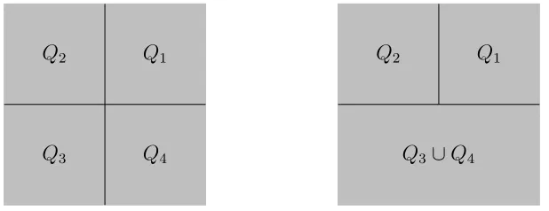
Figure 1.2 The figure on the left shows C, which is a polyhedral complex. The figure on the right shows D, which fails to be a polyhedral complex because Q1 and Q3∪Q4 intersect along a non-face of Q3∪Q4. . . 26

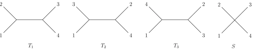
Figure 1.3 Possible tree topologies for a tree metric on four leaves. . . 27

Figure 2.1 The tree on the left has cherries 12 and 56 hence it is a caterpillar. The tree on the right has cherries 12, 34 and 56 and is therefore not a caterpillar. . . 45

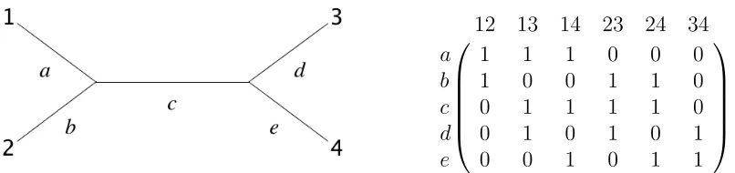
Figure 2.2 Let T be the tree on the left with leaves {1,2,3,4} and edges labels {a, b, c, d, e}. The matrix on the right is AT. Its columns are theλT(ij)’s. 46 Figure 2.3 Breaking T into subtrees. . . 47

Figure 2.4 The caterpillar Cat(n). . . 48

Figure 2.5 K3,3, a Laman graph that is not a basis of M(S2n). . . 51

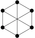
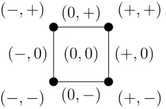
Figure 3.1 Sign vectors corresponding to faces of a square. . . 56

Figure 3.2 Types of x and y with respect toL1 and L2. . . 57

Figure 3.3 L and cubes around (0,0,−1) and (6,4,0). . . 60

Figure 3.4 Two different representations of u= (5,7,9,7,9,9). . . 64

Figure 3.5 Three ultrametrics in C(δ, U4) for δ= (2,4,6,8,10,12). . . 65

Figure 3.6 A 2-dimensional representation of the polyhedral subdivision of _R3 according to district. . . 68

Figure 4.1 AC,d for the HM pair (C,d) in Example 4.1.3. . . 74

Figure 4.2 The complexes P4 (top), J1 (center),J1∗ (left), andJ2 (right). . . 84

Figure 4.3 The complement graphs of P3tK2 and K2tK2tK2. . . 89

(12)

Chapter 1 Introduction

Algebraic statistics is the research area concerned with identifying and exploiting connec-tions between algebraic geometry and statistics. This is a relatively new research area, with its first paper [24] being published in 1998. Since its inception, algebraic statistics has lead not only to new algorithms and research directions in statistics, but in algebraic geometry and and related areas of mathematics as well. For a current sampling of the algebraic statistics landscape, see the textbook-in-press [60].

This thesis solves problems coming from low-rank matrix completion, distance-based phylogenetic reconstruction, and discrete log-linear models. While these applications may seem disjointed, the problems solved therein are unified by the fact that some important underlying structure is a matroid.

Low-rank matrix completion

Chapter 2 concerns the low-rank matrix completion problem. The content of this chapter was published in Linear Algebra and its Applications [6].

(13)

“incoher-ence,” then with high probability, one can use semidefinite programming to recover M from just Θ(n1.25_r_log_{n) entries chosen uniformly at random [17, 18]. These assumptions}

are valid in many applications but another approach is needed for when they are not valid. This motivated Kir´aly, Theran, and Tomioka to develop a new approach using methods of algebraic geometry and matroid theory in 2015 [41], building on a connec-tion with rigidity theory noted by Singer and Cucuringu in 2010 [55]. Improving their approach requires solutions to a slew of interesting mathematical problems, the most basic of which is to characterize the algebraic matroids underlying certain determinan-tal varieties. Chapter 2 gives such a characterization for the case of non-symmetric and skew-symmetric matrices of rank two (Theorems 2.3.2 and 2.3.4). This characterization is obtained by using tropical geometry to translate our question about characterizing this algebraic matroid into a question about phylogenetic trees.

Phylogenetics and linear spaces

Chapter 3 concerns distance-based phylogenetic reconstruction in the l∞-norm and a related problem about linear spaces. The content of this chapter was joint work with Colby Long and it was published in SIAM Journal on Discrete Mathematics [8].

Distance-based methods for phylogenetic reconstruction aim to infer the evolutionary relationships among a set of species from the set of all observed “distances” between each pair. Certain cases admit a geometric interpretation wherein one views their dataset of observed distances as a point in some high-dimensional space and wishes to find the “closest” point that lies within a certain polyhedral complex. Of course, one can choose any metric in which to find this “closest” point. Connections between phylogenetics and tropical geometry [4, 5, 56] suggest that one should investigate the l∞-metric in this context. However, a peculiarity that arises here is that the closest point within this polyhedral complex often fails to be unique. Chapter 3 investigates this failure of uniqueness with the aim of quantifying what is possible.

To begin this investigation, we consider a simpler mathematical question. Namely, given a linear subspace L⊆_Rn _{and a point} _x_∈

Rn, what is the dimension of the subset

ofL consisting of pointsl∞-nearest to x? We then use the (oriented) matroid underlying L to give a polyhedral decomposition of _Rn _{such that any two points in the same cell}

(14)

L if and only if the matroid underlying Lis uniform (Theorem 3.1.9).

Unimodular hierarchical models

Chapter 4 concerns the classification of the unimodular hierarchical models. Part of the content of this chapter was joint work with Seth Sullivant, published in Journal of Combinatorial Theory, Series B [12] and the rest was joint work with Chris O’Neill, published in Journal of Algebraic Statistics [10].

The hierarchical models form a family of discrete log-linear models that are useful for categorical data analysis. In particular, they include the family of discrete graphical models [63]. Such models are naturally indexed by pairs (C,d) where C is a simplicial complex whose ground set is in bijection with the random variables in the model, and

d is a vector giving the number of states of each random variable. One can ask: what useful properties of a hierarchical model can be inferred from the combinatorics of the pair (C,d)?

Chapter 4 investigates one particular property that such a model may satisfy: unimod-ularity. The main result here is a complete classification of all unimodular hierarchical models in terms of the combinatorics of the pairs (C,d) (Theorem 4.9.1). This classifica-tion enables us to give a combinatorial descripclassifica-tion of the Graver basis of any unimodular hierarchical model (Remark 4.10.4). For unimodular hierarchical models, a description of the Graver basis is equivalent to a description of the oriented matroid underlying a particular matrix associated to such a model.

Outline

The remaining sections in this chapter provide the elementary background on a number of concepts that play a prominent role in this thesis. Readers familiar with any of the concepts therein should feel comfortable skipping the corresponding section.

(15)

Section 1.4 and used in Chapters 2 and 3. Tropical geometry is introduced in Section 1.5 and used in Chapter 2. Toric ideals are introduced in Section 1.6 and used in Chapter 4.

1.1 Ideals and varieties

This section gives the required background on algebraic geometry. We expect that the reader has seen most, if not all, of the concepts described here so we proceed rather quickly. All rings in this thesis are assumed to be commutative and unitial. Let _K be a field and let _K[x1, . . . , xn] denote the polynomial ring over K in n indeterminates.

We will use the shorthand xu _:= _xu1

1 · · ·xunn to denote monomials in K[x1, . . . , xn] and K[x] := K[x1, . . . , xn] for the ring itself. Each polynomial f ∈ K[x] defines a function

f :_Kn →_K, sending a:= (a1, . . . , an)∈Kn tof(a) :=f(a1, . . . , an).

Definition 1.1.1. Given a polynomial f ∈_K[x1, . . . , xn], the hypersurface defined by f,

denoted V(f), is defined to be the subset of _Knconsisting of points that evaluate to zero when plugged in to f. That is,

V(f) :={a ∈_Kn :f(a) = 0}.

An affine variety is a (possibly empty) intersection of sets of the formV(f).

We will often drop the qualifier “affine” as all varieties considered will be assumed so unless otherwise stated. We use the shorthandV(f1, . . . , fr) to denoteV(f1)∩· · ·∩V(fr).

Moreover, in cases of a small number of variables, we may substitute different letters for x1, . . . , xn. For example for n= 3, we may write K[x, y, z] instead of K[x1, x2, x3].

Definition 1.1.2. Anideal in a ring R is a subset I ⊆R such that 1. if f, g∈I than f +g ∈I, and

2. if f ∈I and h∈R, then hf ∈I.

Given a subset F of a ring R, we denote byhFi the ideal generated byF. That is, hFi:={g1f1+· · ·+grfr :f1, . . . , fr∈F, g1, . . . , gr ∈R}.

When F ={f1, . . . , fr} is a finite set, we may write hf1, . . . , fri:=hFi. For a fixed ideal

(16)

The following theorem says that every idealI ⊆_K[x] has a finite generating set. A proof can be found in e.g. [32].

Theorem 1.1.3 (Hilbert Basis Theorem). Every idealI ⊆_K[x1, . . . , xn]can be expressed

I =hf1, . . . , fri for somef1, . . . , fr ∈I.

Given a subset S ⊆ _Kn_{, the} _{vanishing ideal of} _{S, denoted} _{I(S), is the set of}

polyno-mials vanishing on S. That is,

I(S) := {f ∈_K[x1, . . . , xn] :f(a) = 0 for all a∈S}.

It is not difficult to see that I(S) is always an ideal. An idealI in a ring R is said to be prime if whenever f g∈I, then either f ∈I or g ∈I.

Example 1.1.4. The ideal hx2_{+ 1i} _{is prime as an ideal in}

R[x]. To see this, note that

x2+ 1 is irreducible as a polynomial in _R[x] and so if f g ∈ hx2_{+ 1i, then either} _f _or _g

must be a multiple ofx2+ 1. In other words, eitherf ∈ hx2_{+ 1i}_or_g _{∈ hx}2_{+ 1i. However,}

hx2 _{+ 1i} _{is not prime as an ideal in}

C[x] since x2+ 1 = (x+i)(x−i) ∈ hx2 + 1i but

neither x+i nor x−i is a member of hx2 _{+ 1i.}

A variety V ⊆ _Kn _{is said to be} _irreducible _if _V _{cannot be expressed as a nontrivial}

union of subvarieties. That is, whenever V = V1∪V2, either V1 =V or V2 =V. If V is

reducible (i.e. not irreducible) then we can expressV =V1∪ · · · ∪Vk where where eachVi

is irreducible. Up to reindexing, this representation is unique and the irreducible varieties V1, . . . , Vk are called the irreducible components of V.

It is not hard to see that V is irreducible if and only if I(V) is prime. Moreover, if V = V1∪V2, then I(V) = I(V1)∩I(V2) and so if the irreducible components of V are

V1, . . . , Vk, thenI(V) = T_kVk.

Example 1.1.5. We consider the geometric side of Example 1.1.4. Note thatV(x2₊₁₎_⊆

C1is a reducible variety sinceV(x2+1) ={−i, i}=V(x+i)∪V(x−i). Moreover,{−i}and

{i}are the irreducible components ofV(x2_{+ 1). Also note that}_hx2_{+ 1i}₌_hx₊_{ii ∩ hx}₋_ii

and that I({−i}) = hx+ii and I({i}) = hx−ii, both of which are prime. Over the reals however, V(x2_{+ 1)}_⊆

R1 is irreducible sinceV(x2+ 1) =∅which clearly cannot be

(17)

Many sets whose geometry we wish to study are not varieties. However, one can still gain insight into such a set by considering its Zariski closure, the smallest variety that contains it. The precise definition is below.

Definition 1.1.6. LetS ⊆_Kn_{be a set. Then the}_{Zariski closure of} _S_{is the set} _V_(I(S)).

Given a variety V ⊆ _Cn _{and a subset} _S _⊆ _V_{, if} _V_{(I(S)) =} _V_{, then we say that} _S _is

Zariski dense in V.

1.1.1 Tangent space and dimension

In this subsection, any unspecified field _K will be assumed to be either _R or _C. Given a point a ∈ _Kn _and _f _∈

K[x1, . . . , xn] we define Da(f) ∈ K[x1, . . . , xn] to be the linear

form given as

Da(f)(x1, . . . , xn) := n

X

i=1

∂f ∂xi

(a)xi.

The affine function La(x1, . . . , xn) :=f(a) +Da(f)(x1−a1, . . . , xn−an) is often known

as the first Taylor approximation to f at a or thelinearization of f at a.

Definition 1.1.7. Given an irreducible variety V ⊆_Kn _{and a point} _a_∈_V_{, the} _tangent

space to V at a is the variety TaV defined as follows

TaV :=V({Da(f) :f ∈I(V)}).

Recall thatV =I(f1, . . . , fr) for somef1, . . . , fr ∈K[x1, . . . , xn] and so eachf ∈I(V)

can be expressed as f = P

igifi. It follows from this, linearity of the partial derivative

operator, the product rule, and fi(a) = 0 for a∈V that

TaV = r

\

i=1

V(Da(fi)).

Since eachV(Da(fi)) is a hyperplane, TaV is a vector subspace of Kn.

Definition 1.1.8. Let _K be either _C or _R and let V ⊆ _Kn _{be an irreducible variety.}

Then the dimension of V, denoted dim(V), to be the smallest dimension of a tangent space of V as a vector subspace of _Kn. That is,

dim(V) := min

(18)

where dim(TaV) is the dimension ofTaV as a vector subspace ofKn. WhenV is reducible,

we define the dimension ofV to be the maximum among the dimensions of the irreducible components of V. That is, if V =V1∪ · · · ∪Vk with eachVi irreducible, then

dimV := max

i dimVi.

The dimension of a variety is more commonly defined as the Krull dimension of its ring of regular functions. This turns out to be equivalent to Definition 1.1.8 - see [28, Chapters 10 and 16].

Example 1.1.9. We now discuss the intuition behind this definition of the dimension of an irreducible variety using V := V(x3 ₋_y2₎ _⊆

C2 as an example (note that it is

irreducible). Let at := (t2, t3) be a point on V and denote f :=x3 −y2. Then Dat(f) is

the linear form on _C2 corresponding to the following row vector

3t2 _2t3_.

ThereforeTatV is defined by the vanishing of this linear form. Whent6= 0, the vanishing

of Dat(V) defines a 1-dimensional subspace of C

2 _{and when} _t _{= 0, the vanishing defines}

the 2-dimensional subspace. Since 1 < 2, V has dimension one. This of course matches our intuition about what the dimension of a curve, such as V, should be.

In Example 1.1.13, we will see why in general it is appropriate to define the dimension of an irreducible variety to be the minimum dimension of any tangent space.

1.1.2 Genericity

In this section, we make repeated use of the following basic fact from linear algebra.

Proposition 1.1.10. Given a matrix A ∈ _Km×n_{, the rank of} _A _is _r _{if and only if all}

(r+ 1)×(r+ 1) subdeterminants ofA vanish and some r×r subdeterminant is nonzero.

Definition 1.1.11. Given an irreducible variety V ⊆ _Kn_{, a property} _P _{is said to hold}

(19)

Example 1.1.12. LetV ⊆_K2×2 _{be the variety defined by the vanishing of the}

determi-nant. That is,

V :=

(

x11 x12

x21 x22

!

:x11x22−x12x21 = 0

)

⊆_K2×2.

Given a matrix A∈V, the rank of A is either 0 or 1. The rank is 0 if and only if A lies in the subvariety U defined by the four additional equations x11 =x12 =x21=x22 = 0.

Hence any matrix inV \U has rank 1 and so we say that a generic point in V is a matrix of rank 1.

More generally, let V ⊆_Km×n _{be the variety defined by the vanishing of all (r}_{+ 1)}_×

(r+ 1) subdeterminants of an m×n matrix of variables. Then the elements ofV are the m×n matrices of rankror less. A generic point of V is a matrix of rankr since in order for a point A ∈ V to have rank r−1 or less, A must lie in the subvariety of V defined by the vanishing of all r×r subdeterminants of an m×n matrix of variables.

Example 1.1.13. When invoking genericity, one is not usually explicit about the par-ticular subvariety they are excluding. For example, consider the following statement:

For generic a ∈V, dimTaV = dimV.

Typically when such a statement is made, the intended audience can easily see that it is true within the complement of some variety. We walk through the above statement to illustrate this. Our definition of the dimension of a variety requires that for any a ∈ V, dimTaV ≥ dimV. Moreover, we established that if V = V(f1, . . . , fr) then TaV can

be computed by intersecting the hypersurfaces defined by the vanishing of the linear formsDa(fi). In other words, if Da(f1, . . . , fr) denotes the r×n matrix whose ij entry is

given by the coefficient of xj in Da(fi), then TaV is simply the kernel of Da(f1, . . . , fn).

Denoting d:= dimV, we can see that the maximum possible rank of rankDa(f1, . . . , fr)

isn−d and that this upper bound is achieved for somea ∈V. Moreover, for any a∈V satisfying dimTaV >dimV, we must have rankDa(f1, . . . , fr)< n−d. In other words,

dimTaV >dimV if and only if a lies in the subvariety of V defined by the vanishing of

(20)

1.2 Matroids

Every chapter in this thesis involves some sort of system that depends on several variables that are intertwined in some way. We will often seek a concise way to describe which subsets of variables constrain each other and which subsets are free. The mathematical object most well-suited for our needs here is thematroid.

Before defining matroids, we give an example demonstrating the type of structure a matroid captures. Consider the matrices A and B shown below, each with columns labeled a, b, c, d

A:=

a b c d

1 2 1 −1

0 0 −1 1

!

B :=

a b c d

2 4 2 4

−1 −2 3 6

!

.

Not only are these matrices different, their rows span different linear subspaces of _R4_.

However, they have the same combinatorial structure in the following sense: no columns are zero and the pairs of column labels corresponding to spanning sets of_R2 _are_{ac, ad, bc,}

and bd. Equivalently, in the subspace of _R4 _{spanned by the rows of each, the pairs of}

coordinates that satisfy a nontrivial linear constraint are those corresponding to the label pairs ab and cd. This underlying combinatorial structure that these two matrices share is what is known as a matroid.

Definition 1.2.1. Let E be a finite set and let I be a set of subsets of E. The pair M:= (E,I) is called a matroid if the following three conditions are satisfied:

1. ∅ ∈ I

2. if J ⊂I and I ∈ I, thenJ ∈ I

3. ifI, J ∈ I with |I|=|J|+ 1, then there exists somee∈I\J such thatJ∪ {e} ∈ I. In this case E is called the ground set of M and the elements of I are called the independent sets of M. Perhaps the simplest matroids are uniform matroids, described below.

Example 1.2.2. Let Ud,n := (E, I) where E is some finite set and I is the set of all

subsets ofE of sizedor less. Then Ud,nis a matroid. Matroids of the formUd,n are called

(21)

Every matrix, graph, and irreducible variety has an underlying matroid. This is some-thing we now explore in detail.

Proposition 1.2.3. Let A ∈ _Km×n _{be a matrix with entries in a field}

K. Let E =

{a1, . . . ,an} be the set of columns of A and let I be the subsets of E that are linearly

independent. Then (E,I) is a matroid.

Proof. It is clear that (E,I) satisfies the first two requirements to be a matroid so we now show that it satisfies the third. Let I, J ⊆ E be linearly independent sets with |I|=|J|+ 1. Let L, M be the linear subspaces of_Km with bases given byI and J. For a given e∈I\J, the setJ∪ {e} is dependent if and only ife lies inM. But if every e∈I lies in M, thenL⊆M which cannot happen because dim(L) = dim(M) + 1.

Definition 1.2.4. For a given matrixA, the matroid that arises as in Proposition 1.2.3 is called the(linear) matroid underlyingA, denotedMA. A matroidMsatisfyingM=MA

for some _K-matrix A is called_K-representable, or representable over _K.

There do exist matroids that are not representable over any field _K (see e.g. [49, Proposition 2.2.26]) but we will not be concerned with such matroids in this thesis.

Example 1.2.5. Every uniform matroid Ud,n is Q-representable. In particular, if A ∈ Qd×n is a d×n matrix such that no d×d sub-determinant vanishes, then MA = Ud,n.

However, a givenUd,n may not beK-representable for certain finite fieldsK. For example,

U2,4 is notF2-representable. If it were, then suppose A∈F2d×4 had MA=U2,4. Then we

could assume d= 2 since the rank of A must be 2. But there are exactly four vectors in

F22, so either a column ofAgets repeated, or (0,0) is a column. Either way, the underlying

matroid will not be uniform.

Proposition 1.2.6. Let G = (V, E) be a graph with edge set E. Let I be the subsets of E that do not have any cycle. Then (E,I) is a matroid.

Proof. Fix a total ordering≺ on the vertex setV. LetA≺_G be the matrix whose rows are indexed byV, whose columns are indexed byE, and whose (v, e) entry is 0 ifeis a loop, 1 if v is the ≺-minimal vertex of e, −1 is the ≺-maximal vertex of v, and 0 otherwise. We now show thatI is the set of independent sets in M_A≺

G.

Given S ⊆E, let AS denote the submatrix of A≺G consisting of the columns indexed

(22)

of AS that has exactly one non-zero entry corresponding to a vertex s of degree one in

the graph (V, S). This implies that any vector x giving linear dependenceASx= 0 must

satisfy xs = 0. Therefore the columns of AS are linearly dependent if and only if the

columns of AS\{s} are too. However, the columns of AS\{s} are linearly independent by induction.

It now remains to show that if S ⊆ E has a cycle, then AS has linearly dependent

columns. So assume S contains a cycle C = v1, v2, . . . , vk, v1. Define x ∈ KS so that

xe = 0 ife does not appear in the cycle, xe= 1 if e={vi, vj} withi < j and vi ≺vj and

xe =−1 if e={vi, vj} with i < j but vi vj. Then ASx= 0.

Definition 1.2.7. For a given graph G, the matroid that arises as in Proposition 1.2.6 is called the (polygon) matroid underlying G, denoted MG. A matroid M satisfying

M=MG for some graph Gis called graphic.

It is clear from the proof of Proposition 1.2.6 that each graphic matroid is repre-sentable over any field _K. However, there do exist matroids that are representable, but not graphic. For example,U2,4 is not graphic and this follows from the fact that it is not

F2-representable.

Example 1.2.8. LetGbe the graph shown below and let≺order the vertices according to their integer labels. then the independent sets ofMGare all proper subsets of{b, c, d}.

One can check that these are also the independent sets of M_A≺

G.

1 2

3

b c

d a

A≺_G=



 

a b c d

1 0 1 0 1

2 0 0 1 −1

3 0 −1 −1 0



 .

The last class of matroids we will encounter come from irreducible varieties. In the following proposition we use the notation _KE _{to denote the}

K-vector space whose

coor-dinates are in some natural bijection withE, which will be a finite set.

Proposition 1.2.9. Let _K be _R or _C and let E be a finite set. Let V ⊆ _KE _{be an}

(23)

Proof. For a givenx∈V, let TxV denote the tangent space ofV atx. For genericx∈V,

the projection of V onto_KS _{is full-dimensional if and only if the projection of} _T

xV onto KS is full-dimensional. Therefore it suffices to prove the proposition in the case that V

is a linear space. Now let V be the row span of some matrix A∈_Kn×|E| _{whose columns} are indexed by E. Then the projection of V onto _KS _{is full-dimensional if and only if}

the columns of A corresponding to the elements of S are linearly independent. It then follows from Proposition 1.2.3 that (E,I) is a matroid.

Definition 1.2.10. For a given irreducible varietyV in_Rnor_Cn, the matroid that arises as in Proposition 1.2.9 is called the (algebraic) matroid underlying V, denoted MV.

In the proof of Proposition 1.2.9, we saw that the algebraic matroid underlying a real or complex irreducible variety is the same as the algebraic matroid underlying a generic tangent space. Moreover, the algebraic matroid underlying a linear space is simply the column matroid of a certain matrix. HenceM=MV for some irreducible real or complex

variety V if and only if Mis _R- or _C-representable, respectively.

Example 1.2.11. Let E ={a, b, c, d}. If V is the variety in the space with coordinates labeled byE defined by the two polynomials below, thenMV is the same as the matroid

MG from Example 1.2.8

a−1 = 0 b2+ 3c3−d+ 1 = 0.

The algebraic matroid underlying a variety is usually formulated in terms of algebraic independence in the corresponding function field (see e.g. Section 6.7 in [49]). For varieties defined over _R or _C, either definition leads to the same class of matroids, which as we already remarked, are simply the _R- or _C-representable matroids. However, in order to define the algebraic matroid underlying a variety over a finite field, one must use this definition in terms of algebraic independence in the function field. For finite fields, this actually leads to a larger class of matroids, but we chose to present the algebraic matroid in terms of projections because it is more geometrically intuitive, and we will only be considering _R and _C as base fields anyway.

(24)

Definition 1.2.12. Let M = (E,I) be a matroid. A circuit of M is a subset C ⊆ E such that C is not independent in M, but every proper subset is.

Example 1.2.13. LetG= (V, E) be a graph. The circuits in the matroidMGunderlying

G are precisely the subsets of E that support a cycle.

By definition, the independent sets of a matroid determine the circuits. The converse is also true. Namely, given the ground set E of a matroidMand its setC of circuits, the independent sets are simply the subsets of E that do not contain a circuit. In this way, the circuits and the independent sets of a matroid carry the same structure. In fact, due to the following proposition, one can even axiomatize matroid theory in terms of circuits instead of independent sets.

Proposition 1.2.14. Let E be a finite set and letC ⊆ 2E be a set of subsets of E. Then C is the set of circuits of a matroid on ground set E if and only if

1. ∅∈ C/

2. if C1 ⊆C2 then C1 =C2

3. if C1 6=C2, then for any e∈C1∩C2, there exists C3 ∈ C such that

C3 ⊆(C1∪C2)\ {e}.

For a proof of Proposition 1.2.14, see [49, Chapter 1.1]. We end this section by noting several other structures one often associates with a matroid. A basis of M is an inde-pendent set of maximum cardinality. Therank function of Mis the functionρ: 2E →_N that sends a given S ⊆ E to the cardinality of the largest independent set contained in S. For a given S ⊆E, we often refer to ρ(S) as the rank of S. The rank of M is simply ρ(E), the rank of the ground set. A spanning set of Mis a superset of a basis.

Example 1.2.15. LetMbe the matroid shown in Examples 1.2.8 and 1.2.11. The bases of Mare {b, c},{b, d}and {c, d}, and the circuits are {a} and {b, c, d}. The sets of rank zero are ∅and {a}. The sets of rank one are {b},{c},{d},{a, b},{a, c},{a, d}. The other nine subsets of {a, b, c, d} have rank 2 and are spanning sets.

(25)

1.3 Oriented matroids

Given a matroid coming from a matrix with entries in an ordered field (usually _R) or a graph with directed edges, there is some extra structure that one can add on to the underlying matroid. A matroid equipped with this extra structure is called an oriented matroid. We begin with some examples. Consider the two following real matrices

a b c

1 1 −1

1 −1 0

!

and

a b c

1 1 1

1 −1 0

!

.

Both have the same underlying matroid; in particular, {a, b, c} is the unique circuit of both. Any linear dependence corresponding to this circuit in the first matrix is in the subspace spanned by (1,1,2), while such a dependence for the second is in that of (1,1,−2). In particular, any linear dependence of the first matrix has sign pattern (+,+,+) or (−,−,−) whereas any linear dependence of the second matrix has sign pattern (+,+,−) or (−,−,+). The oriented matroids associated to each of these matrices is what captures this difference.

One can also define an oriented matroid corresponding to a directed graph which cap-tures information that the underlying matroid misses. For example, consider the following two directed graphs.

a

c b

a

c b

(26)

We now introduce the formal definitions needed to define an oriented matroid. Let E be a finite set. A sign vector is an element of the set {0,+,−}E_{; that is, an assignment}

of either 0,+ or − to each element of E. Given u∈_RE_{, sign(u) denotes the sign vector}

obtained by replacing each entry of u with its sign. We will often assume an ordering on the elements of E, in which case can write a sign vector as (s1, . . . , s|E|). Given a

sign vector σ = (σ1, . . . , σ|E|), we define −σ := (−σ1, . . . ,−σ|E|) according to the rules

−− = +, −+ =−, and −0 = 0. The composition of two sign vectors σ and τ, denoted σ◦t is defined by

(σ◦τ)e=







σe if σe 6= 0

τe otherwise

.

Note that foru, v ∈_Rn_{, sign(u}₊_{εv) = sign(u)}_◦_{sign(v) when} _ε_{is sufficiently small. The}

separation set for sign vectorsσ, τ is defined by

S(σ, τ) := {e∈E :σe=−τe 6= 0}.

Forf ∈S(σ, τ), we say that ρeliminates f between σ and τ if

ρf = 0 and ρe= (σ◦τ)e for all e /∈S(σ, τ).

Note that for u, v ∈ _RE _satisfying _u

e = 1 and ve = −1, sign(u+v) eliminates i across

sign(u) and sign(v).

Definition 1.3.1. Let V be a set of sign vectors for E. Then the pair O := (E,V) is said to be an oriented matroid if the following four conditions are satisfied:

1. (0, . . . ,0)∈ V

2. if σ ∈ V then −σ∈ V 3. if σ, τ ∈ V then σ◦τ ∈ V

4. if σ, τ ∈ V with f ∈S(σ, τ), there exists ρ∈ V that eliminates f between σ and τ. In this case, the set V of sign vectors is called the vectors of O and E is called the ground set. These four conditions are often called the (co)vector axioms of an oriented matroid. We will often abuse notation and terminology, identifying the set of vectors of

(27)

the same ground set, we may similarly write O ⊆ P to mean that every vector of the oriented matroid O is also a vector of the oriented matroidP.

We now detail how one can obtain an oriented matroid from any linear subspace of _Rn_{. For any real number} _r _∈

R, sign(r) ∈ {+,−,0} is the sign of r. For a linear

functionalc∈(_Rm₎∗_{, sign(c)}_{∈ {+,}_−,_0}m _{is defined by sign(c)}

i = sign(ci). Given a sign

vector σ∈ {+,−,0}m_{, we define} _|σ|_:=_|supp(σ)|.

Proposition 1.3.2. Let L ⊆ _Rm _{be a linear subspace. Let} _V _{be the set of sign vectors}

σ ∈ {+,−,0}m _{such that} _σ_{= sign(c)} _{for some linear functional} _c_∈₍

Rm)∗ vanishing on

L. Then ([m],V) is an oriented matroid.

Proof. It is clear that the first two vector axioms are satisfied. Let cσ and cτ be linear functionals vanishing on L such that sign(cσ) = σ and sign(cτ) = τ. For small enough ε > 0, sign(cσ ₊_εcτ_{) =} _σ _◦ _τ _{thus showing that the third vector axiom is satisfied.}

Choosee∈S(σ, τ). By scaling appropriately, we can choosecσ

e =−cτe. Then sign(cσ+cτ)

eliminates e betweenσ and τ thus showing that the fourth vector axiom is satisfied. For a linear space L ⊆ _Rm _{we refer to the oriented matroid of Proposition 1.3.2 as}

the oriented matroid associated to L, denoted OL. LetA ∈Rm×n be a matrix. Then we

may refer to OrowA, the oriented matroid underlying the row-span of A, as the oriented

matroid underlying the columns of A. This is reasonable because it consists of all sign patterns of dependencies among the columns ofA. WhenO =OLfor someL, we simplify

notation and write ML instead of MOL. Note that this is consistent with our notation

for the algebraic matroid underlying an irreducible variety (linear spaces are irreducible varieties).

Example 1.3.3. LetA =1 1 0

and letL= rowA⊆_R3_{. Denote the coordinates of}

the underlying space_R3 _as_{x, y} _and _{z. Linear functionals that vanish on} _L_include_x₋_y,

3z, and 2x−2y−z. It is not hard to see that the vectors in O, the oriented matroid underlying L (equivalently, the oriented matroid underlying the columns of A), are the following

(28)

Let ≺∗ _{be the partial order on}_{+,_−,_0}_{given by 0} _≺∗ _{+ and 0}_≺∗ ₋ _{with + and} ₋ incomparable. Then ≺ is the partial order on {+,−,0}m _{that is the Cartesian product}

of ≺∗ _m _{times. The} _{(signed) circuits} _{of an oriented matroid} _O _{are the nonzero vectors} of O that are minimal with respect to ≺. A consequence of the following proposition is that in order to completely specify an oriented matroid, it suffices to specify its set of circuits.

Proposition 1.3.4. Let O be an oriented matroid. Given σ ∈ O, there exist signed circuits τ1, . . . , τk such that σ=τ1◦ · · · ◦τk.

Proof. Let {τ1_{, . . . , τ}k_} _{be the set of all signed circuits satisfying} _τ _≺ _{σ. For each} _i ₌

1, . . . , k and each e ∈ E, either τ_ei = σe or τei = 0. Therefore τ1 ◦ · · · ◦τk ≺ σ. It now

suffices to show that for each e ∈ supp(σ), there exists some circuit τ ≺ σ satisfying τe = σe. Let τ ∈ O be the support-minimal vector such that τ ≺ σ and τe =σe. If τ is

not a circuit, then there exists some circuitρ≺τ withρe = 0. Then letηbe a vector that

eliminates some f ∈ S(τ,−ρ) between τ and −ρ. Then ρ◦η contradicts the minimality of τ; note that (ρ◦η)e =ηe 6= 0, ρ◦η≺τ and ρ◦η6=τ since (ρ◦η)f = 0 6=τf.

Example 1.3.5. The oriented matroid OL from Example 1.3.3 has four circuits which

are (0,0,+),(+,−,0), and their negatives. Note that we can represent any zero non-circuit as a composition of two non-circuits. For example, (+,−,+) = (+,−,0)◦(0,0,+).

The support of a sign vector σ, denoted supp(σ), is defined to be the set {e ∈ E : σe 6= 0}. Lemma 1.3.6 below will be used to prove Proposition 1.3.7, which justifies the

name “oriented matroid.”

Lemma 1.3.6. Given a sign vector τ ∈ {+,−,0}E_{, if there exists some} _σ _{∈ O} _with

σ 6=±τ and supp(σ)⊆supp(τ), then τ is not a signed circuit.

Proof. If τ /∈ O, then τ is trivially not a signed circuit, so assume τ ∈ O. We proceed by induction on min|S(±σ, τ)|, which we assume without loss of generality is |S(σ, τ)|. For the base case, note that since supp(σ) ⊆ supp(τ), S(σ, τ) = ∅ implies that σ ≺ τ, thus showing that τ is not a circuit. So assume there exists e ∈ S(σ, τ) and let ρ ∈ O eliminate e between σ and τ. Then ρ satisfies supp(ρ)⊆ supp(τ) and S(ρ, τ)₍S(σ, τ). So by induction on min|S(±σ, τ)|, τ is not a circuit.

(29)

Proof. We proceed by showing that {supp(σ) : σ ∈ C} satisfies the conditions given in Proposition 1.2.14. That {supp(σ) : σ ∈ C} satisfies the first condition follows from the fact that circuits are defined to be nonzero. That they satisfy the second condition follows from Lemma 1.3.6.

We now show the third condition. Let C1 = supp(σ) and C2 = supp(t) and assume

C1 6=C2 with e ∈ C1∩C2. Since supp(σ) = supp(−σ), we may assume that σe = −τe.

Then the fourth axiom of oriented matroids implies that there exists some ρ ∈ V that eliminates between e between σ and τ. Let η ρ be a signed circuit. Then supp(η) ⊆ (C1∪C2)\ {e} and so we can take C3 = supp(η).

We call the matroid of Proposition 1.3.7 the matroid underlying O. The rank of any sign vector σ with respect to O, is the rank of supp(σ) in MO. Note that this is well defined for any sign vector, not just those in O.

Example 1.3.8. We return once again to the oriented matroid from Example 1.3.3. The matroid underlyingOL has three independent sets, which are ∅,{1} and{2}. The ranks

of the three sign vectors in the bottom row of the table in Example 1.3.3 are all zero, and the ranks of the other six are all one.

We now describe how one can obtain an oriented matroid from a directed graph. Let G= (V, A) be a directed graph with vertex setV and arc setA. Let C be a cycle in the undirected graph underlying G. We will now show how C gives rise to two sign vectors σC and τC. For each arc a ∈A whose corresponding undirected edge does not lie in C, set σa = τa = 0. There are exactly two cyclic orientations of C which we denote C+

and C−. For each arc a ∈A whose corresponding edgee lies in C, set σa = −τa = + if

the orientation C+ _{imposes on} _e _{agrees with} _{a, and set}_σ

a =−τa =−otherwise. Define

CG :=S_C{σC, τC}.

Proposition 1.3.9. For a directed graph G= (V, A), the set CG is the set of circuits of

an oriented matroid OG.

Proof. LetMG be the matrix whose rows are indexed by V, whose columns are indexed

by A, and whose entry corresponding to a pair (v, a) is 1 if a emanates from v, −1 if a points towards v, and 0 otherwise. Then note that the set of signed circuits of the oriented matroid underlying the row-span ofMG isCG. ThereforeCG is the set of circuits

(30)

For a directed graph G, we refer to the oriented matroid OG from Proposition 1.3.9

as the oriented matroid underlying G.

Example 1.3.10. Consider the directed graphG shown below a

b

c

d e

Ordering the arcs as (a, b, c, d, e), one can check that the circuits ofOG are the following

sign vectors and their negatives:

(+,+,0,0,+) (+,+,+,−,0) (0,0,+,−,−).

1.3.1 Oriented matroid duality

Definition 1.3.11. Let E be a finite set. Given two sign vectors σ, τ ∈ {+,−,0}E_{, we}

say thatσ, τ are orthogonal and write σ·τ = 0 if one of the following holds 1. for each e∈E, σe = 0 orτe = 0, or

2. there exist e, f ∈E such thatσe =τe 6= 0 andσf =−τf 6= 0.

Given a set of sign vectors S ⊆ {+,−,0}E_{, we define the} _{orthogonal complement of} _S _as

S⊥ :={τ ∈ {+,−,0}E :σ·τ = 0 for allσ ∈S}.

Example 1.3.12. Consider the following two examples

(+,0,0,−)·(+,0,−,+) = 0 but (+,0,0,+)·(+,0,−,+) 6= 0.

For the first case, note that if x = (1,0,0,−1) and y = (1,0,−1,1), then x·y = 0, sign(x) = (+,0,0,−), and sign(y) = (+,0,−,+). However, for the second case, note that if x, y satisfy sign(x) = (+,0,0,+) and sign(y) = (+,0,−,+), thenx·y > 0. More generally, one can see that two sign vectorsσ, τ ∈ {+,−,0}E _satisfy _σ_·_τ _{= 0 if and only}

if there exist x, y ∈_RE _satisfying _x_·_y_{= 0, sign(x) =}_{σ, and sign(y) =}_τ_.

(31)

Definition 1.3.13. Let O = (E,V) be an oriented matroid. Then the dual oriented matroid of O is

O∗ := (E,V⊥).

Example 1.3.14. Consider the oriented matroid O given in Example 1.3.3. Then the dual oriented matroid O∗ _{contains exactly two nonzero vectors, both of which are signed} circuits. They are (+,+,0) and (−,−,0).

For a proof of the following proposition, see e.g. [15].

Proposition 1.3.15. Given an oriented matroid O = (E,V), the dual oriented matroid O∗ _{is an oriented matroid. Moreover,} _O∗∗₌_O.

When an oriented matroid O underlies a linear subspace L⊆_Rn _{or a directed graph}

G, then the dual oriented matroids O∗

L and O

∗

G can be constructed explicitly. We begin

with linear spaces.

Definition 1.3.16. LetA ∈ _Rr×n _{be a matrix of rank} _{r. A} _{Gale dual} _of _A _{is a matrix}

B ∈_R(n−r)×n _{of rank}_n₋_r _{such that} _ABT _{= 0.}

Note that if B is a Gale dual of A, then A is a Gale dual ofB. We now show that if A and B are Gale duals, then O∗_A=OB.

Proposition 1.3.17. Let A ∈ _Rr×n _{be a matrix of rank} _r _{and let} _B _{be a Gale dual of}

A. Then O∗

A=OB.

Proof. Let σ ∈ OB and let x ∈ Rn such that Bx = 0 and sign(x) = σ. Now let y ∈ Rn

such that Ay = 0. Since the columns of BT _{are a basis of ker}_A, _y ₌ _BT_z _{for some}

z ∈ _Rn−r_{. Then} _xT_y ₌ _xT_BT_z _{= 0 which implies sign(x)}_·_σ _{= 0. This implies that}

σ ∈ O∗

A and therefore OB ⊆ OA∗.

By making an analogous argument with the roles of A and B reversed we see that OA ⊆ O∗B. Note that for any two collections of sign vectorsS,T, ifS ⊆ T, thenT

⊥_{⊆ S}⊥ . Therefore we have O∗

A⊆ O

∗∗

B =OB.

Example 1.3.18. Let A be the matrix from Example 1.3.3. We display A alongside a Gale dual B below

A=1 1 0

B = 1 −1 0

0 0 1

!

(32)

We saw in Example 1.3.14 that the dual oriented matroid O∗

A has exactly two nonzero

vectors which are (+,+,0) and (−,−,0). This is exactly the oriented matroid underlying B, whose kernel is spanned by AT_.

We now discuss the combinatorial interpretation of the circuits in oriented matroids that are dual to those underlying directed graphs. When dealing with oriented matroids underlying graphs, it tends to be more natural to work with circuits than with vectors so we begin with the following proposition.

Proposition 1.3.19. Let O = (E,V) be an oriented matroid and let C ⊆ V denote its set of circuits. Then V⊥₌_C⊥_.

Proof. It is clear that V⊥ _{⊆ C}⊥ _{so we prove the other direction. Let} _σ _{∈ C}⊥ _{and let} τ ∈ V. Assumeτ /∈ C so that τ =τ1_{◦ · · · ◦}_τk_{. As} _τ

1 ∈ C,σ·τ1 = 0. There are two cases

to consider. The first case is that σe = 0 whenever τe1 6= 0. From this and the inductive

hypothesis, it follows that (τ2 _{◦ · · · ◦}_τk₎_·_σ _{= 0, which in turn implies} _τ _·_σ _{= 0. The}

second case is that there exist e, f ∈ E such that σe = τe1 6= 0 and σf = −τf1 6= 0. This

immediately implies τ·σ = 0.

Definition 1.3.20. Let G = (V, E) be a graph on vertex set V and edge set E. A cut of G is a subset C ⊆ E of edges such that the subgraph (V, E \C) has strictly more connected components than G. A bond of G is an inclusion-minimal cut.

Note that any bond C of an undirected graph G = (V, E) will separate exactly one connected component of Ginto two connected components in (V, E\C). We denote the subgraphs induced on these connected components by G1 = (V1, E1) and G2 = (V2, E2).

So each edgee∈C is incident to exactly one vertex in eachVi. WhenGis the undirected

graph underlying some directed (V, A), we create a sign vector σ∈ {+,−,0}A _{such that}

σe = 0 for all e /∈ C, σe = + if e ∈ C and e is oriented from V1 to V2, and σe = − if

e∈C and e is oriented from V2 toV1. Note that changing the roles ofV1 andV2 negates

the corresponding sign vector.

Definition 1.3.21. For a directed graph G = (V, A), any sign vector in {+,−,0}A

obtained as described above is called a signed bond of G.

Proposition 1.3.22. Let G = (V, A) be a directed graph. The set of signed bonds of G is the set of circuits in O∗

(33)

Proof. Letσbe a signed bond ofG. Since signed bonds are support-minimal by definition, it only remains to show that σ ∈ O∗

G. By Proposition 1.3.19, it suffices to show that

σ·τ = 0 for every signed circuit τ of G. So let G1 = (V1, E1) and G2 = (V2, E2) be the

new connected components of (V, A\supp(σ)). Assume σ was specified so that σe = +

whenever e points from V1 into V2. Let τ ∈ OG. Then if σe = τe = + (without loss

of generality), this means that as we traverse the cycle supp(τ) according to τ, we are moving from V1 into V2 at the edge e, which means we must move back from V2 into V1

at some other edgef. Iff points fromV1 toV2 we would haveτf =−andσf = + and if

f points from V2 into V1, then we would have τf = + and σf =−. Either way, σ·τ = 0.

Now we must show that the circuits of O∗_G are signed bonds. So let σ∈ O_G∗. First we claim that supp(σ) is a cut in the undirected graph underlying G. To see this, note that for any cycle C of this graph, |supp(σ)∩C| 6= 1. Now if e∈supp(σ) has endpointsv, w, then every path between v and w in the undirected graph underlying G must have an edge in supp(σ). Otherwise, ifv, x1, x2, . . . , xk, w is a path fromv towwithxi ∈/ supp(σ),

then the cycle obtained by adding the edge e back to this path is a cycle that intersects supp(σ) in exactly one element, namelye.

Now since the support of each σ ∈ O∗

G is a cut, supp(σ) must contain a bond. We

have already seen that each bond ofG is the support of some vector (moreover a circuit) in O_G∗, so if we assume that σ is a circuit, then Lemma 1.3.6 implies that σ is a signed bond ofG.

Example 1.3.23. Let G be the directed graph from Example 1.3.10. Again, ordering the arcs as (a, b, c, d, e), we see that the signed bonds of G are the vectors shown below, along with their negatives. Note that these are the circuits of the dual oriented matroid O∗

G.

(+,−,0,0,0) (+,0,−,0,−) (0,0,+,+,0) (0,+,0,+,−) (0,+,−,−,0) (+,0,0,+,−)

1.4 Tree metrics

(34)

of the set of all tree metrics.

1.4.1 Basic definitions

Let X be a finite set. A dissimilarity map on X is a functiond :X×X →_R such that d(x, y) = d(y, x) and d(x, x) = 0. We will usually associate each dissimilarity map d on X with the point d∈_R([n2]) given by d

xy =d(x, y).

Definition 1.4.1. A tree metric on X is a dissimilarity map d ∈ _R(X2) satisfying the

following four point condition for all distinctx, y, z, w ∈X dxy +dzw≤max{dxz+dyw, dxw+dyz}.

This is equivalent to the condition that the maximum ofdxy+dzw, dxz+dyw, anddxw+dyz

is attained twice.

Other authors often define tree metrics to be the dissimilarity map satisfying the four point condition, not just for sets of four distinct points, but additionally in cases where there is overlap among them. The reason for this is that the four point condition becomes the triangle inequality when only three of the four points are distinct, and it ensures non-negativity of each dxy when only two are. Therefore, this more restrictive

definition ensures that tree metrics are indeed metrics. In spite of this, we take this less restrictive definition because it makes the set of all tree metrics into the tropicalization of a particular variety, a fact we later exploit. Proposition 1.4.3 justifies the terminology “tree metric.”

Definition 1.4.2. A tree is a connected graph T = (V, E) with no cycles. A leaf of a tree is a vertex of degree one and aninternal edge is an edge that is not incident to any leaf. Given a finite set X, an X-tree is a tree with leaf set X that has no vertices of degree two. A tree isbinary if all internal vertices have degree three.

Proposition 1.4.3 ([53, Chapter 7]). Let T = (V, E) be an X-tree and let ω : E → _R be a weighting of the edges of T such that ω(e) ≥ 0 for all internal edges of T. Let dω

T :X×X →R be the dissimilarity map defined by

dω_T(x, y) =X

e∈P

(35)

1

2 3

4 −1

1

2

−3

Figure 1.1: An edge-weighted tree with positive internal edge weights whose leaves are labeled by {1,2,3,4} showing that d = (d12, d13, d14, d23, d24, d34) = (0,3,−2,5,0,−1) is

a tree metric.

where the sum is taken over the edges in the unique path from x to y in T. Then d is a tree metric. Moreover, for every tree metric d, there is a unique X-tree T = (V, E) and edge weighting ω satisfying ωe 6= 0 for all e∈E such that d=dωT.

When one takes the alternate definition of tree metric that requires the four point condition for allx, y, z, w ∈X, and not just those that are distinct, then Proposition 1.4.3 is still true, but all edge weights are required to be nonnegative, not just the internal ones. The uniqueness of the tree specified in the second part of Proposition 1.4.3 gives us a combinatorial invariant of a tree metric.

Definition 1.4.4. Let d be a tree metric on X. The unique tree T from Proposition 1.4.3 is called the (tree) topology of d.

Example 1.4.5. LetX = [4] and let d be the dissimilarity map given as (d12, d13, d14, d23, d24, d34) = (0,3,−2,5,0,1).

Note that d12 +d34 = 1, and d13 +d24 = d14 +d23 = 3 and so the maximum of the

three sums is attained twice. Hence d satisfies the four point condition and is therefore a tree metric. Moreover, if T is the tree displayed in Figure 1.1 with the indicated edge weighting ω, thend=dω_T.

(36)

1.4.2 Polyhedral geometry of the space of tree metrics

A polyhedral cone is the intersection of finitely many linear half-spaces. That is, an intersection of finitely many sets of the form{x∈_Rn_:_ax_≥_{0}. Note that the intersection}

of any two polyhedral cones is also a polyhedral cone. Given a polyhedral cone C ⊆_Rn_,

a face is a subset F ⊆C of the form

F ={x∈C :cx= 0}

for some c∈ (_Rn₎∗ _{such that} _cx_≥ _{0 for all} _x_∈_{C. Note that every face of a polyhedral} cone is itself a polyhedral cone. Setting c = 0, we see that the entire cone C is a face of itself. A proper face of C is any face other than C itself An inclusion-maximal proper face is called a facet.

Definition 1.4.6. A polyhedral fan is a set C of polyhedral cones in _Rn _{satisfying the}

following two conditions

1. if C ∈ C and F is a face of C, thenF ∈ C

2. if C, D ∈ C, then C∩D is a face of bothC and D.

The elements of C are called the faces of C and the inclusion maximal faces are called facets.

Example 1.4.7. Fori= 1,2,3,4, letQi denote the ith quadrant ofR2 and letAi denote

the rotation of the ray {(x,0) :x≥0} by 90(i−1) degrees counter-clockwise about the origin. Define

C :={Q1, Q2, Q3, Q4, A1, A2, A3, A4,{0,0}}

and

D:={Q1, Q2, Q3∪Q4, A1, A2, A3, A1∪A3,{0,0}}.

Both C and D satisfy the first condition required of a polyhedral fan. Figure 1.2 displays the maximal elements of both C and D. However, only C satisfies the second -note that (Q3∪Q4)∩Q1 =A1 which is a face of Q1 but not of (Q3 ∩Q4).

The support of a polyhedral fan C is S := S

C∈CC. In this situation, we say that S supports C. The polyhedral fan structure supported on a givenS ⊆_Rn _{is in general not}

(37)

Q1

Q2

Q3 Q4

Q1

Q2

Q3∪Q4

Figure 1.2: The figure on the left shows C, which is a polyhedral complex. The figure on the right shows D, which fails to be a polyhedral complex because Q1 and Q3 ∪Q4

intersect along a non-face of Q3∪Q4.

so is the polyhedral fan {_R2_{}. The set of all tree metrics on [n] naturally supports a}

polyhedral fan structure which we now describe.

Definition 1.4.8. LetTndenote the polyhedral fan structure supported on the set of all

tree metrics on [n] that has a face CT for every [n]-tree T, consisting of all tree metrics

with topology T0 such that T0 can be obtained from T via a (possibly empty) sequence of internal edge contractions.

The facets of Tn are the faces corresponding to the binary [n]-trees. We will often

abuse notation and identify the polyhedral fan Tn with its support.

Example 1.4.9. We consider the polyhedral structure of T4 in detail. A tree metric on

leaf set {1,2,3,4} can have one of four topologies, displayed in Figure 1.3. The binary tree topologies will be denoted T1, T2, and T3 and the nonbinary tree topology will be

denoted S. ThusT4 has three facets, each consisting of all the tree metrics with topology

S orTi for somei= 1,2,3. The intersection of any two facets is the set of all tree metrics

with topology S.

1.5 Tropical geometry

Tropical geometry gives us a way to transform an irreducible variety V ⊆ _Cn _{into a}

polyhedral complex trop(V) ⊆ _Rn_{, called the} _{tropicalization of} _V_{, that encodes many}

(38)

1 2 3 4 T1 1 3 2 4 T2 1 4 2 3 T3 1 2 3 4 S

Figure 1.3: Possible tree topologies for a tree metric on four leaves.

We consider two equivalent ways one can define the tropicalization of a varietyV ⊆_C. For one of these ways, the first step is to consider V over a certain field extension of_C, called thefield of Puiseux series. This field is naturally endowed with a valuation, which is a particular kind of function into_Q. By applying this function coordinate-wise to every point inV, one obtains a rational subset of_Rn_{, the Euclidean closure of which is trop(V}_).

This view of trop(V) is well-suited for proving certain theorems, and in particular, that trop(V) caries the algebraic matroid structure ofV. One can equivalently define trop(V) to be the set of pointsω ∈_Rn_{such that the initial ideal}_in

ω(I(V)) contains no monomials.

This definition is well-suited for computing tropical varieties.

1.5.1 Puiseux series

Definition 1.5.1. A Puiseux series is a formal power series with rational exponents with coefficients in_C such that the set of all exponents of the formal variable is bounded below, and expressible over a common denominator. That is, a Puiseux series is a formal power series of the form P

α∈Jd,kcαt

α _where _d _∈

N and k ∈ Z and Jd,k = {n/d : n ∈ Z, n ≥ k}. Addition and multiplication of formal power series induces the structure of

an algebraically closed field on the set of Puiseux series [45, Theorem 2.1.5]. We denote this field by _C{{t}}. The valuation map is the function val : _C{{t}} → _Q that sends a Puiseux series to its minimum exponent.

Example 1.5.2. Consider the following three formal power series

f := ∞

X

n=−8

ntn/3 g := ∞

X

n=1

t−n h:= ∞

X

n=1

t1/n.

(39)

have that val(f) = −8/3. The issue with g is that its set of exponents is not bounded below. The issue with h is that its exponents cannot all be expressed over a common denominator.

Definition 1.5.3. Let V ⊆ _Cn _{be a variety and let (}

C{{t}} ⊗V) ⊆ (C{{t}})n denote

the variety defined by the ideal I(V)_C{{t}}[x1, . . . , xn]. Let val : (C{{t}})n → Rn

de-note the map sending each (a1, . . . , an) ∈ (C{{t}})n to (val(a1), . . . ,val(an)). Then the

tropicalization of V is

trop(V) := (−1)·val(_C{{t}} ⊗V),

the Euclidean closure of the image of_C{{t}}⊗V under the negation of the coordinate-wise valuation map val. Sets of the form trop(V) are called tropical varieties.

One often defines the tropicalization of a variety in almost the same way, but with-out taking negatives at the end (see e.g. the introductory text [45]). Both conventions result in the same theory, modulo some trivial sign and order differences. Our motivation for choosing the convention that takes negatives is that it makes the connection with phylogenetics cleaner.

Example 1.5.4. Letf(x, y) =x2+xy+y−1. Note that the variety _C{{t}} ⊗V(f(x, y)) contains the points (t−1,−t−1_{+ 1) and (−1, t}2_{). Applying the coordinate-wise valuation}

map val to each point gives us (−1,−1) and (0,2). Therefore, their negations (1,1) and (0,−2) lie in the tropical variety trop(V(f(x, y)). In the next section, we will develop tools that will enable us to describe the entire set trop(V(f(x, y)).

1.5.2 Initial ideals

Definition 1.5.5. Letf =P

α∈J cαxα be a polynomial inK[x1, . . . , xn] and letω ∈Rn.

Define

Jω :={α∈ J :ω·α is maximized over J }.

The initial form of f with respect to ω is the polynomial inωf :=

X

α∈Jω

(40)

Given ω∈_Rn _{and an ideal}_I _⊆

K[x], theinitial ideal of I with respect to ω is

inωI :=hinωf :f ∈Ii.

IfI =hf1, . . . , fri, it is clear thathinωf1, . . . , inωfri ⊆inωI. However, the converse is

false in general as the following example shows.

Example 1.5.6. Define f1(x1, x2, x3) :=x1 −x2 and f2(x1, x2, x3) := x1−x3 and let I

denote the ideal they generate in_K[x1, x2, x3]. Letω= (3,2,1). Theninωf1 =inωf2 =x1

and so hinωf1, inωf2i = hx1i. However, this cannot be the whole initial ideal because

x2 ∈inωI asinω(x2 −x3) =x2 and x2−x3 ∈I.

Definition 1.5.7. LetI ⊆_K[x1, . . . , xn] be an ideal and letω ∈Rn. A set of polynomials

f1, . . . , fr ∈I is called a Gr¨obner basis forω if

inωI =hinωf1, . . . , inωfri.

One might be concerned about the fact that Gr¨obner bases are not required by defi-nition to generate the ideal they correspond to. However, this property is an easy conse-quence of the definition. Given an arbitrary generating set of an ideal, one can compute a Gr¨obner basis with respect to anyω∈_Rn_using_{Buchberger’s algorithm. For more details,}

see e.g. [32, Chapter 2]. Initial ideals and Gr¨obner bases are particularly important for tropical geometry due to the following theorem which gives an alternate characterization of the tropicalization of a variety.

Theorem 1.5.8([45], Theorem 3.2.3). LetV ⊆_Cn _{be a variety. Then the tropicalization}

of V is the set of all ω ∈_Rn _{such that the corresponding initial ideal of} _in

ωI(V) contains

no monomials. That is,

trop(V) ={ω ∈_Rn_:_in

ωI(V) contains no monomials}.

Example 1.5.9. Consider the polynomial f(x, y) = x2 ₊_xy ₊ _y₋ _{1 from Example}

1.5.4. Given ω ∈ _R2_{, the initial ideal} _in

ωhf(x, y)i contains no monomials if and only if

inωf(x, y) is itself not a monomial. By way of case analysis over all pairs of monomials

of f(x, y), one can see that inωf(x, y) is not a monomial when ω1 = 0, or ω1 ≥ 0 and

ω2 =ω1, or ω1 ≤0. Theorem 1.5.8 then implies that trop(V(f(x, y)) is the union of the

(41)

1.5.3 Algebraic matroids and tropical geometry

As we noted earlier, the tropicalization of an irreducible variety V carries with it the structure of the algebraic matroid underlying V. This section makes that statement precise. All unspecified fields _Kin this subsection are assumed to be _R or _C.

Definition 1.5.10. Let V ⊆ _KE _{be a set. The} _{independence complex of} _V_{, denoted}

M(V), is the set of subsets S ⊆ E such that the coordinate projection of S onto _KS _is

full-dimensional in _KS_.

When V ⊆_KE _{is an irreducible variety,} _M_(V_{) is the set of independent sets of} _M V,

the algebraic matroid underlying V. When V is an arbitrary set,M(V) need not be the independent sets in any matroid.

Proposition 1.5.11([64], Lemma 2). LetV ⊆_CE _{be an irreducible variety. Then}_S _⊆_E

is independent in the algebraic matroid MV underlyingV if and only ifS ∈M(trop(V)).

The utility of Proposition 1.5.11 is that computing the dimension of a projection of a tropical variety may be easier than computing the dimension of the projection of the variety itself. This is because a tropical variety is a highly structured polyhedral complex. We will wait until Chapter 2 to make this statement precise. For now, we give an example.

Example 1.5.12. LetE = [4]₂ be the set consisting of all pairs of integers 1,2,3,4. Let V ⊆_CE _{be the variety defined by the following polynomial}

p12p34−p13p24+p14p23.

It is not hard to see directly that the algebraic matroid underlying V is simply the uniform matroid U5,6, but we prove this using Proposition 1.5.11.

Since I(V) is generated by a single polynomial, an initial ideal inωI(V) contains a

monomial if and only if inω(p12p34−p13p24+p14p23) is a monomial. Moreover, such an

initial form is a monomial if and only ifωsatisfies the four point condition. Therefore, the tropicalization trop(V) is T4, the set of all tree metrics on leaf set {1,2,3,4}. There are

three distinct binary tree topologies on four leaves and each corresponds to a maximal cone in T4. The linear hull of each such maximal cone is the linear space spanned by the