Learning from Domain Complexity
Robert Remus
†, Dominique Ziegelmayer
‡†Natural Language Processing Group, University of Leipzig, Germany
‡Institut f¨ur Informatik, University of Cologne, Germany
[email protected],[email protected]
Abstract
Sentiment analysis is genre and domain dependent, i. e. the same method performs differently when applied to text that originates from different genres and domains. Intuitively, this is due to different language use in different genres and domains. We measure such differences in a sentiment analysis gold standard dataset that contains texts from 1 genre and 10 domains. Differences in language use are quantified using certain language statistics, viz. domain complexity measures. We investigate 4 domain complexity measures: percentage of rare words, word richness, relative entropy and corpus homogeneity. We relate domain complexity measurements to performance of a standard machine learning-based classifier and find strong correlations. We show that we can accurately estimate its performance based on domain complexity using linear regression models fitted using robust loss functions. Moreover, we illustrate how domain complexity may guide us in model selection, viz. in deciding what wordn-gram order to employ in a discriminative model and whether to employ aggressive or conservative wordn-gram feature selection.
Keywords:Domain complexity; model selection; sentiment analysis
1.
Introduction
Sentiment Analysis (SA) is—just like natural language pro-cessing in general (Sekine, 1997; Escudero et al., 2000)—
genre and domain dependent (Wang and Liu, 2011), i.e. the same SA method performs differently when applied to different genres and domains. Intuitively, this is due to dif-ferent language usein differentgenres1anddomains2. In this paper, we measure such differences in an SA gold standard dataset that contains texts from 1 genre—product reviews—and 10 domains, e. g. apparel and music. Differ-ences in language use are quantified using certain language statistics, viz.domain complexity measures.
We relate domain complexity to performance of a standard Machine Learning (ML)-based classifier and find strong correlations. We show that we can accuratelyestimate its performance based on domain complexity. Moreover, we illustrate how domain complexity may guide us in model selection.
1.1. Related Work
Related to our work are Ponomareva and Thelwall (2012), who estimate—using domain complexity and domain similarity—the accuracy loss when transferring an SA method from a source to a target domain. Van Asch and Daelemans (2010) estimate—using domain similarity—the accuracy loss when transferring a part of speech-tagger from one domain to another. Blitzer et al. (2007) compute anA-distance proxy and show that it correlates with accu-racy loss when transferring their SA method from a source to a target domain.
1Agenreis an identifiable text category (Crystal, 2008, p. 210)
based on external, non-linguistic criteria such as intended audi-ence, purpose, and activity type (Lee, 2001) as well as textual structure, form of argumentation, and level of formality (Crystal, 2008, p. 210).
2
Adomainis a genre attribute that describes the subject area that an instantiation of a certain genre deals with (Steen, 1999; Lee, 2001).
1.2. Outline
This paper is structured as follows: In Section 2. we de-scribe domain complexity measures that we use to quantify differences in language use. In Section 3. we relate domain complexity to performance and show what we can learn
from their relationship. In Section 4. we conclude and point out directions for future work.
2.
Domain Complexity
Domain complexityis a measure that “reflects the difficulty of [a] classification task for a given data set” (Ponomareva and Thelwall, 2012). We use 4 approximations of domain complexity: 3 approximations proposed by Ponomareva and Thelwall (2012) and 1 proposed by Remus (2012).
2.1. Ponomareva and Thelwall (2012)
Ponomareva and Thelwall (2012) proposed 3 measures as approximations of domain complexity:
Percentage of rare words. The percentage of rare words is defined as in Equation (1)
P RW =|{w∈W |c(w)<3}|
|W| (1)
where W is the vocabulary, vocabulary size |W|
equals the number of types, i. e. the number of dif-ferent words in a text sample, andc(w)is the number of occurrences ofwin a text sample.
Word richness. The word richness is defined just as the
type/token ratioT T Rin Equation (2)
T T R= P |W|
w∈Wc(w)
(2)
whereP
w∈Wc(w)equals the number oftokens, i. e.
Table 2: Pearson correlationr between domain complex-ity measurements and accuracies of SVM models based on word unigrams as well asr’s significance levelp.
Domain complexity measure r p
Percentage of rare unigrams -0.673 0.023 Unigram type/token ratio -0.723 0.012 Unigram relative entropy -0.425 0.192 Unigram homogeneity -0.708 0.015
tuation characters are removed. From hereon we refer to this classifier asour SA method.
All classification experiments arebinaryand construed as 10-fold CVs. In each fold 9/10th of the available data are used for training, the remaining 1/10th is used for testing. Training and testing data never overlap. As performance measure we reportaccuracyA.
3.1. Performance Estimation
In this section we relate differences in domain complex-ity of an SA gold standard dataset to differences in perfor-mance of our SA method evaluated on the same SA gold standard dataset. Table 1 depicts the differences in perfor-mance when we evaluate our SA method—viz. SVM mod-els based on word unigrams, uni- and bigrams, and uni-, bi-, and trigrams—on different domains from MDSD v2.0. Table 1 also depicts the differences in domain complexity of the same domains.
We correlate the accuracies achieved by our SVM mod-els based on word unigrams and the corresponding do-main complexity measurements. Table 2 shows the results. All correlations—except of unigram relative entropy—are strong (|r|>0.67) and statistically significant (p <0.05). From Table 2 we learn that
• the smaller the percentage of rare unigrams, i. e. the less hapax legomena and dis legomena,
• the smaller the unigram type/token ratio, i. e. the more tokens per type,
• the smaller the unigram relative entropy, i. e. the far-ther the distribution from a uniform distribution and
• the smaller the unigram homogeneity value, i. e. the more homogeneous the corpus,
the higher the accuracy of our SA method.
Given such strong correlations, we perform an ordinary Linear Regression (LR) using squared error loss with single domain complexity measurements aspredictors6 and sin-gle accuracies asresponses. We measure the mean resid-ual standard error (MRSE) of the LR models in leave-one-domain-out CVs7.
6
We do not use more than one predictor in our LR models in accordance with Harrell (2001, p. 61), who suggests to obey the rule of thumbp < n/10wherepis the number of predictors
andnis the total sample size. In our leave-one-domain-out CV experimentsn= 9(and hence1>9/10).
7Leave-one-(domain)-out CV (Hastie et al., 2009, p. 242) is a
special case of aK-fold CV, whereK =nandnis the number
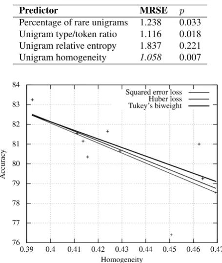
Table 3: MRSEs of ordinary LR models fitted using squared error loss in leave-one-domain-out CVs with do-main complexity measurements as predictors and accura-cies of SVM models based on word unigrams as responses.
Predictor MRSE p
Percentage of rare unigrams 1.238 0.033 Unigram type/token ratio 1.116 0.018 Unigram relative entropy 1.837 0.221 Unigram homogeneity 1.058 0.007
76 77 78 79 80 81 82 83 84
0.39 0.4 0.41 0.42 0.43 0.44 0.45 0.46 0.47
Accurac
y
Homogeneity
Squared error loss Huber loss Tukey’s biweight
Figure 1: Accuracy of an SVM model based on word uni-grams vs. unigram homogeneity plus LR models fitted us-ing squared error loss, Huber loss, and Tukey’s biweight.
Table 3 shows the resulting MRSEs as well as the signifi-cance levelpof the predictor’s influence on the response. All predictors’ influences on the response—except of un-igram relative entropy—are statistically significant (p <
0.05).
From Table 3 we learn that—analogously to the correla-tions we found—3 out of 4 domain complexity measures allow us to accurately estimate our SA method’s perfor-mance based solely on domain complexity measurement. Unigram homogeneity appears to be the most informative domain complexity measure: it yields the smallest MRSE (1.058).
As we can see in Figure 1 our data contains (at least) one outlier: the domain MUSICwith an accuracy of 76.4 and a unigram homogeneity of 0.451. Outliers such asMUSIC
affect the slope of the LR fit. We counteract outliers by em-ploying loss functions that are more robust than ordinary squared error loss: Huber loss (Huber, 1964) and Tukey’s biweight (Holland and Welsch, 1977). Using these robust loss functions in LR leads to small improvements in esti-mating accuracy—i. e. reduces the MRSEs—as shown in Table 4.
Figure 1 depicts LR models fitted to our data using squared
of instances—e. g. domains—in the data: we fit a model ton−1
parts of the data and validate it on the held outn-th part. Then
Table 1: Accuracies on MDSD v2.0 of SVM models based on word unigrams, uni- and bigrams, or uni-, bi-, and trigrams as well as domain complexity measurements.
Domain Our SA method’s accuracy Domain complexity measure
uni uni, bi uni, bi, tri P RW T T R Hrel Hom APPAREL 83.25 85.55 85.05 0.6801 0.4294 0.8891 0.3923
BOOKS 79.25 79.65 79.5 0.7261 0.4595 0.8871 0.4640
DVD 78.55 79.8 79.25 0.7244 0.4631 0.8897 0.4695
ELECTRONICS 80.65 82.05 81.6 0.6916 0.4409 0.8888 0.4292
HEALTH 80.35 83.55 83.45 0.6813 0.4306 0.888 0.4156
KITCHEN 81.15 82.1 81.85 0.6857 0.4369 0.8879 0.4137
MUSIC 76.4 78.45 78.9 0.7175 0.4600 0.8926 0.4507
SPORTS 81.65 83 82.95 0.687 0.4361 0.88789 0.4240
TOYS 81.55 83.15 82.75 0.6765 0.4308 0.8916 0.4112
VIDEO 81 81.65 81.65 0.7248 0.4618 0.8882 0.4624
Table 4: MRSEs of robust LR models fitted using Huber loss and Tukey’s biweight in leave-one-domain-out CVs with domain complexity measurements as predictors and accuracies of SVM models based on word unigrams as re-sponses.
Predictor Huber Tukey’s
Percentage of rare unigrams 1.205 1.208 Unigram type/token ratio 1.054 1.073 Unigram relative entropy 1.959 2.050 Unigram homogeneity 1.027 1.082
error loss, Huber loss, and Tukey’s biweight. Both robust LR models are less influenced by outliers. Thus, they result in a more accurate fit of the data, especially when applied to subsamples of the data as in our leave-one-domain-out CVs.
Performance estimation does not only work for SVM mod-els based on word unigrams, but also for SVM modmod-els based on higher order word n-grams, i. e. SVM models based on word uni- and bigrams and SVM models based on word uni-, bi-, and trigrams: we just use higher order word n-gram domain complexity measurements as addi-tional predictorsin our LR models. E. g., to estimate the accuracy of an SVM model based on word uni- and bi-grams, we measure both word unigram relative entropy and word bigram relative entropy, or both unigram type/token ratio and bigram type/token ratio etc. These additional pre-dictors are either kept separatelyoraveraged. Averaging predictors, e. g. averaging word uni-, bi-, and trigram rela-tive entropy, results in a single predictor in our LR models. Keeping predictors separately results in multiple predictors in our LR models.
We then proceed as described earlier. Results of the accu-racy estimation for SVM models based on word uni- and bigrams are shown in Table 5. Results of the accuracy es-timation for SVM models based on word uni-, bi-, and tri-grams are shown in Table 6.
For accuracy estimation of SVM models based on word uni- and bigrams using percentage of rare words as separate (i. e. not averaged) predictors and an LR model fitted using Tukey’s biweight yields the smallest MRSE (0.472). For accuracy estimation of SVM models based on word uni-,
Table 5: MRSEs of LR models fitted using squared er-ror loss, Huber loss, and Tukey’s biweight in leave-one-domain-out CVs with domain complexity measurements as predictors and accuracies of SVM models based on word uni- and bigrams as responses. “sep” denotes separately kept predictors, “avg” denotes averaged predictors.
Predictor(s) Squared Huber Tukey’s
P RW sep 0.94 0.506 0.472
avg 0.963 0.905 0.907
T T R sep 0.942 0.591 0.579
avg 0.921 0.777 0.765
Hrel
sep 0.902 0.882 0.87 avg 1.604 1.514 1.464
Hom sep 1.02 1.063 1.067
avg 0.927 0.925 0.958
Table 6: MRSEs of LR models fitted using squared er-ror loss, Huber loss, and Tukey’s biweight in leave-one-domain-out CVs with domain complexity measurements as predictors and accuracies of SVM models based on word uni-, bi-, and trigrams as responses. “sep” denotes sepa-rately kept predictors, “avg” denotes averaged predictors.
Predictor(s) Squared Huber Tukey’s
P RW sep 1.143 0.867 0.738
avg 0.913 0.943 0.928
T T R sep 1.048 0.747 0.634
avg 0.781 0.713 0.75
Hrel
sep 1.002 1.022 1.049 avg 1.43 1.429 1.620
Hom sep 1.037 0.996 0.904
avg 0.877 0.854 0.894
bi-, and trigrams using type/token ratio as separate (i. e. not averaged) predictors and an LR model fitted using Tukey’s biweight yields the smallest MRSE (0.634).
Discussion
Table 7: Accuracies of our model selector for wordn-gram model order. “1–2” denotes first vs. second order, “2–3” denotes second vs. third order. “sep” denotes separately kept predictors, “avg” denotes averaged predictors.
Predictor(s) Squared Huber Tukey’s
1–2 2–3 1–2 2–3 1–2 2–3
P RW sep 100 80 90 90 70 80 80 50 65
avg 100 80 90 100 70 85 100 40 70
T T R sep 90 90 90 90 80 85 90 80 85
avg 100 80 90 100 60 80 90 40 65
Hrel
sep 60 80 70 60 70 65 60 70 65
avg 90 80 85 90 70 80 80 60 70
Hom sep 100 80 90 100 80 90 90 70 80
avg 100 80 90 100 90 95 90 90 90
e. g. whether the gold standard dataset contains erroneous labels, its size, and its class boundary complexity (Ho and Basu, 2002).
3.2. Model Selection: Wordn-gram Model Order
In this section, we let domain complexity guide us in model selection, viz. in deciding what word n-gram model or-der to employ in our SA method for a given domain from MDSD v2.0. For example, we decide whether to employ a first order SVM model based on word unigrams, or a sec-ond order SVM model based on word uni- and bigrams for MDSD v2.0’s domainHEALTH.
An algorithm for model selection, viz. amodel selector es-timates the accuracies ofn-th (n≥1) order SVM models for a given domain as described in Section 3.1. The model selector then chooses the SVM model that yields the high-est high-estimated accuracy as shown in Pseudocode 3.
Pseudocode 3: Model selector for wordn-gram model or-der.
1 input: dataset
2 for n = 1, 2, ..., k {
3 estimate accuracy of an SVM model based on word {1,
..., n}-grams on dataset
4 }
5 output: n that yields the highest estimated accuracy
3.2.1. Evaluation
We evaluate our model selector in a leave-one-domain-out CV on MDSD v2.0’s 10 domains, in which for each run we train our model selector on 9 domains and decide what word n-gram model order to employ in an SVM for the remaining 1 domain.
Data We decide between first, second and third order wordn-gram models, i. e. between SVM models based on word unigrams, word uni- and bigrams, or word uni-, bi-, and trigrams. To produce data for our leave-one-domain-out CV, we evaluate 3 SVM models per domain in 10-fold CVs: one SVM model based on word unigrams, one SVM model based on word uni- and bigrams and one SVM model based word uni-, bi-, and trigrams. The evaluation results are shown in Table 1. SVM models based word uni- and bigrams always outperform SVM models based solely on word unigrams. SVM models based on word uni-, bi-, and trigrams outperform SVM models based on word uni- and bigrams only for 1 domain:MUSIC.
Experiments We vary 3 parameters of our model selec-tor’s accuracy estimation. (i) We compare 4 predictors: percentage of rare words, type/token ratio, relative entropy, and homogeneity. (ii) We compare separately kept and av-eraged predictors. (iii) We compare 3 LR loss functions: squared error loss, Huber loss, and Tukey’s biweight. Eval-uation results of our leave-one-domain-out CV are shown in Table 7.
Results Our model selector yields an average accuracy between 60–100 when deciding between first or second or-der. It yields an average accuracy between 40–90 when deciding between second or third order. It yields an overall accuracy between 65–95.
The most reliable model selector uses averaged homogene-ity as predictor and fits the LR model using Huber loss: it yields an average accuracy of 100 when deciding be-tween first or second order. It yields an average accuracy of 90 when deciding between second or third order. Thus, it yields an overall average accuracy of 95.
Note that for our data a na¨ıvebaselinealso yields an overall average accuracy of 95: a na¨ıve model selector thatalways
decides for second order yields an average accuracy of 100 when deciding between first or second order. It yields an average accuracy of 90 when deciding between second or third order. Thus, its overall average accuracy is also 95.
3.3. Model Selection: Aggressive vs. Conservative Wordn-gram Feature Selection
In this section we let domain complexity guide us in an-other model selection, viz. in deciding whether to employ aggressive or conservative wordn-gram feature selection in our SA method for a given domain from MDSD v2.0. We face 2 questions when we perform wordn-gram feature se-lection:
1. Which feature selection method should we use?
2. How many features should we select?
We answer question 1 up front: as feature selection method we use Information Gain (IG) (Yang and Pedersen, 1997), because it has been shown that IG is superior to other fea-ture selection methods for wordn-gram based text classifi-cation (Yang and Pedersen, 1997; Forman, 2003).
Table 8: Accuracies of SVM models based on word uni-grams with (w/) and without (w/o) feature selection via IG based on the ideal CO in percent (and word unigram types).
Domain w/o w/ ∆ CO
APPAREL 83.25 83.6 0.35 78% (7,927)
BOOKS 79.25 80.45 1.2 11% (3,136)
DVD 78.55 80.55 2 60% (18,169)
ELECTRONICS 80.65 81.75 1.1 85% (13,139)
HEALTH 80.35 80.85 0.5 90% (11,778)
KITCHEN 81.15 82.8 1.65 17% (2,214)
MUSIC 76.4 78.45 2.05 2% (506)
SPORTS 81.7 82.55 0.85 19% (2,715)
TOYS 81.5 82.45 0.95 4% (564)
VIDEO 81.05 81.6 0.55 80% (20,301) average 80.39 81.51 1.12 45% (8,044)
Table 9: Pearson correlationrbetween ideal CO and do-main complexity measurements as well asr’s significance levelp.
Domain complexity measure r p
Percentage of rare word unigrams -0.08 0.814 Word unigram type/token ratio -0.119 0.727 Word unigram relative entropy -0.35 0.291 Word unigram homogeneity -0.095 0.78
3.3.1. Evaluation
As in Section 3.2.1. we evaluate our model selector—which we develop in our experiments—in a leave-one-domain-out CV.
Data Feature selection methods such as IG produce an implicit ranking with the most predictive features ranked highest and the least predictive features ranked lowest. To employ feature selection via IG we have to determine acut off (CO): features ranked above the CO are kept, while fea-tures ranked below the CO are discarded.
To produce data for our leave-one-domain-out CV for each domain we determine the CO for which our SVM model’s accuracy peaks. First we rank a domain’s word unigrams via IG. We then set the CO to 1, 2, . . . , 100% of the do-main’s original word unigram vocabulary size. If it is set to 1% we keep its 1% highest ranked word unigrams, if it is set to 2% we keep its 2% highest ranked word unigrams etc. For each of the resulting 100 word unigram vocabularies we evaluate an SVM model based on this word unigram vocab-ulary in a 10-fold CV. We call the CO for which our SVM model’s accuracy peaksideal CO. Table 8 shows evalua-tion results of SVM models based on word unigrams with and without feature selection via IG. Feature selection is based on the ideal CO.
With feature selection using the ideal CO average accuracy is 1.12 higher than without feature selection. Ideal COs are scattered, with 85% (13,139 word unigram types) being the most conservative feature selection and 2% (506 word unigram types) being the most aggressive feature selection. The average ideal CO is 45% (8,045 word unigram types).
Experiments Table 9 correlates domain complexity mea-surements of MDSD v2.0’s 10 domains with their ideal CO.
0.887 0.888 0.889 0.89 0.891 0.892 0.893
0 10 20 30 40 50 60 70 80 90
Relati
v
e
entrop
y
Ideal CO in % LR model
Figure 2: Ideal CO vs. relative entropy.
Table 10: Ideal COs and COs estimated by our model se-lector fitted using Huber loss as well as accuracies of SVM models using feature selection based on ideal and estimated CO.
Domain Ideal Estimated
CO A CO A
APPAREL 78% 83.6 41% 83.50
BOOKS 11% 80.45 74% 78.25
DVD 60% 80.55 38% 80.10
ELECTRONICS 85% 81.75 42% 80.45
HEALTH 90% 80.85 46% 80.50
KITCHEN 17% 82.8 59% 82.30
MUSIC 2% 78.45 39% 77.65
SPORTS 19% 82.55 60% 81.75
TOYS 4% 82.45 37% 81.00
VIDEO 80% 81.6 47% 80.00
average 45% 81.51 48% 80.55
Relative entropy correlates strongest with ideal CO (-0.35): the smaller the domain’s relative entropy, the larger its ideal CO. Hence, the less uniform a domain’s word unigram dis-tribution, the more of its word unigrams are kept as features in our SVM model. Figure 2 plots relative entropy vs. ideal CO. Additionally, it shows an LR model fitted to the data using squared error loss. It achieves no perfect fit, but it still roughly estimates ideal CO.
Given its correlation with the ideal CO, we use as our model selector a robust LR model with relative entropy as single predictor and ideal CO as response. We compare LR mod-els fitted using Huber loss and Tukey’s biweight. Table 10 shows the evaluation results of our leave-one-domain-out CV for Huber loss, Table 11 shows the evaluation results for Tukey’s biweight.
se-sentiment analysis. InProceedings of the International Conference of the German Society for Computational Linguistics and Language Technology (GSCL), number 8105 in LNCS, pages 176–183. Springer.
Robert Remus. 2012. Domain adaptation using domain similarity- and domain complexity-based instance selec-tion for cross-domain sentiment analysis. In Proceed-ings of the 2012 IEEE 12th International Conference on Data Mining Workshops (ICDMW 2012) Workshop on Sentiment Elicitation from Natural Text for Information Retrieval and Extraction (SENTIRE), pages 717–723. Satoshi Sekine. 1997. The domain dependence of parsing.
InProceedings of the 5th Conference on Applied Natural Language Processing (ANLP), pages 96–102.
Gerard Steen. 1999. Genres of discourse and the definition of literature.Discourse Processes, 28(2):109–120. Vincent Van Asch and Walter Daelemans. 2010. Using
do-main similarity for performance estimation. In Proceed-ings of the 2010 Workshop on Domain Adaptation for Natural Language Processing (DANLP), pages 31–36. Vladimir Vapnik. 1995. The Nature of Statistical Learning.
Springer New York, NY.
Dong Wang and Yang Liu. 2011. A cross-corpus study of unsupervised subjectivity identification based on cal-ibrated EM. In Proceedings of the 2nd Workshop on Computational Approaches to Subjectivity and Sentiment Analysis (WASSA), pages 161–167.