Learning Based Java for Rapid Development of NLP Systems
Nick Rizzolo, Dan Roth
University of Illinois at Urbana-Champaign {rizzolo,danr}@illinois.edu
Abstract
Today’s natural language processing systems are growing more complex with the need to incorporate a wider range of language resources and more sophisticated statistical methods. In many cases, it is necessary to learn a component with input that includes the predictions of other learned components or to assign simultaneously the values that would be assigned by multiple components with an expressive, data dependent structure among them. As a result, the design of systems with multiple learning components is inevitably quite technically complex, and implementations of conceptually simple NLP systems can be time consuming and prone to error. Our new modeling language, Learning Based Java (LBJ), facilitates the rapid development of systems that learn and perform inference. LBJ has already been used to build state of the art NLP systems. This paper details recent advancements in the language which generalize its computational model, making a wider class of algorithms available.
1.
Introduction
As the fields of Natural Language Processing (NLP) and Computational Linguistics have matured, more sophisti-cated language resources and tools have become available. These tools perform complicated analyses of natural lan-guage text to find named entities, identify the argument structure of verbs, determine the referents of pronouns and nominal phrases, and more. Many such tasks involve mul-tiple learning components whose collective objective is to assign values to variables that may have an expressive, data dependent structure among them. Thus, systems that per-form these tasks have complicated, data dependent develop-ment cycles and run-time interactions. As such, their imple-mentations become large and unwieldy, which can restrict their usefulness as resources.
Organized infrastructure solutions such as GATE (Cun-ningham et al., 2002), NLTK (Loper and Bird, 2002), and IBM’s UIMA (G¨otz and Suhre, 2004) only partially solve these issues. They aim to make separately learned compo-nents “plug-and-play”, but they do not help manage their training nor do they offer solutions when the outputs of dif-ferent components contradict each other. The more recently developed Alchemy (the most popular MLN (Richardson and Domingos, 2006) implementation) and FACTORIE (McCallum et al., 2009) systems offer general purpose so-lutions for global training and inference, but they lack the flexibility to decompose the problem, and general purpose algorithms quickly become intractable on the large prob-lems encountered in NLP.
A comprehensive solution for modeling problems in NLP (as well as other domains) would combine the advantages of both types of systems mentioned above. It would make effortless the combination of arbitrary types of components in the learned system, be they learned or hard coded (e.g. features and constraints). At the same time, it would al-low the modeling of large, structured problems over which learning and inference can be performed globally. How-ever, in contrast to the systems above, it should also allow a flexible decomposition of such large, structured problems so that learning and inference can be efficiently tailored to suit the problem.
We refer to the whole of these principles as Learning Based Programming (LBP) (Roth, 2006). Our previous work in-troduced Learning Based Java1 (LBJ) (Rizzolo and Roth,
2007), a modeling langauge that represented a first step in this direction. It modeled a user’s program as a collection of locally defined experts whose decisions are combined to make them globally coherent. While this is certainly one type of decomposition LBP aims to provide, the language lacked the expressivity to specify other interesting models.
This paper makes three main contributions. First, we demonstrate that there exists a theoretical model that de-scribes most, if not all, NLP approaches adeptly (Section 2.). Second, we describe our improvements to the LBJ language and show that they enable the programmer to de-scribe the theoretical model succinctly (Sections 3. and 4.). Third, we introduce the concept of data driven compilation, a translation process in which the efficiency of the gener-ated code benefits from the data given as input to the learn-ing algorithms (Section 5.). Thus, the programmer spends his time designing his models instead of worrying about the low level details of writing efficient learning based pro-grams that have been abstracted away.
2.
A Model for NLP Systems
We submit the constrained conditional model (CCM) of (Chang et al., 2008) as the paradigmatic NLP modeling framework. A CCM can be represented by two weight vec-tors, w and ρ, a set of feature functions Φ = {φi|φi :
X × Y → R}, and a set of constraintsC = {Cj|Cj :
X × Y →R}. Here,X is referred to as the input space and Y is referred to as the output space. Most often, both are multi-dimensional. LetXbe the set of possible values for a single element of the input, and letΥbe similarly defined for the output. ThenX = Xp andY = Υq for integersp andq.
The score for an assignment to the output variablesy∈ Y on an input instancex ∈ X can then be obtained via the
1
1. model ArgumentIdentifier :: discrete[] input -> boolean isArgument
2. input[*] /\ ˆisArgument;
3. model ArgumentType :: discrete[] input -> discrete type
4. input[*] /\ type;
5. input[*] /\ input[*] /\ type;
6. static model pertinentData :: ArgumentCandidate candidate
7. -> discrete[] data
8. data.phraseType = candidate.phraseType(); 9. data.headWord = candidate.headWord(); 10. data.headTag = candidate.headTag();
11. data.path = candidate.path();
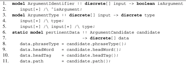
Figure 1: The SRL system from Section 2.2. is decomposed into two learned components whose general structure is defined in lines 1-5. Lines 6-11 define a hard-coded model that collects data from a Java object for later use as input variables for the learned components.
2.3. Other CCMs in the Wild
Examples of more complicated CCMs abound in the NLP literature. (Barzilay and Lapata, 2006) describes an au-tomatic semantic aggregator that uses constraints to con-trol the number of aggregated sentences and their lengths. (Marciniak and Strube, 2005) describes a general constraint framework for solving multiple NLP problems simultane-ously. (Martins et al., 2009) describes a dependency pars-ing system that incorporates prior knowledge as hard con-straints. These and other systems would be more easily maintainable, more portable, and more useful as resources if they had been developed in a modeling formalism de-signed specifically for them. We aim to provide such an environment in Learning Based Java.
3.
Learning Based Java
Learning Based Java has already been used to develop sev-eral state-of-the-art resources. The LBJ POS tagger2
re-ports a competitive 96.6% accuracy on the standard Wall Street Journal corpus. In the named entity recognizer of (Ratinov and Roth, 2009), non-local features, gazetteers, and wikipedia are all incorporated into a system that achieves 90.8F1 on the CoNLL-2003 dataset, the highest score we are aware of. Finally, the co-reference resolution system of (Bengtson and Roth, 2008) achieves state-of-the-art performance on the ACE 2004 dataset while employing only a single learned classifier and a single constraint.
Nevertheless, our previous work on LBJ was not expres-sive enough to represent features involving multiple output variables. This paper redesigns LBJ to represent, learn, and perform inference over arbitrary CCMs. We introduce our modeling language by example. The codes in Figures 1, 2, and 3 specify the structure of the Punyakanok, et al. se-mantic role labeling system.3 These figures discuss how LBJ language constructs address the concerns of the SRL system as described in Section 2.2. Section 3.1. discusses each in turn. Section 3.2. then describes the syntax of fea-tures and constraints in more detail.
2
http://L2R.cs.uiuc.edu/∼cogcomp/software.php
3Some of the features and constraints have been omitted to save space.
3.1. Models
A model in LBJ simply represents an objective function of the form of equation (1) in which the weightsw are im-plicit (recall thatρis specified by a human; thus it is ex-plicit). Features and constraints are specified in a logic syn-tax as described in Section 3.2. Once these are specified, the model can be instantiated so that each instance contains its own weight vectors.
Decomposition: Figure 1 immediately describes the unit of decomposition used to build the system. The two models declared on lines 1 and 3 are the models that will do all the system’s learning. TheArgumentIdentifiermodel will be a linear threshold unit, so it has abooleanoutput vari-able. Its body declares features in the form of equation (3). TheArgumentTypemodel will be a multi-class classifier, so it has adiscreteoutput variable. Its features are de-clared in the form of equation (5). (The syntax for writing these features on lines 2, 4, and 5 is described in Section 3.2.) Finally, Figure 1 declares a model used merely to ex-tract the data we wish to utilize in these learned models. We will see in Figure 3 how this data is given to them.
In more detail, a model declaration’s header contains a name for the model and a list of argument specifications. The list is partitioned by an arrow (->) indicating that the arguments on the left represent input, and the arguments on the right represent output variables. Input may mean input variables, primitive types, or Java objects from the programmer’s main program. The variables (either input or output) in these examples are the ones with typesboolean ordiscrete. They are intended precisely to represent the
xandyinput and output variables in equation (1).
Any model may be declared static, and it has roughly the same meaning as the same keyword when used on a Java method. Models with no learnable parameters are usually declared static. A model may also be hard-coded, though there is no keyword for this property. A hard-coded model is one whose output is well defined even without learn-ing any parameters. The pertinentDatamodel on line 6 which contains only assignment statements is both static and hard-coded.
1. static model noOverlaps :: ArgumentCandidate[] candidates -> discrete[] types
2. for (i : (0 .. candidates.size() - 1))
3. for (j : (i + 1 .. candidates.size() - 1))
4. #: candidates[i].overlapsWith(candidates[j]) 5. => types[i] :: "null" || types[j] :: "null";
6. static model noDuplicates :: -> discrete[] types
7. #: forall (v : types[0].values)
8. atmost 1 of (t : types) t :: v;
9. static model referenceConsistency :: -> discrete[] types
10. #: forall (value : types[0].values)
11. (exists (var : types) var :: "R-" + value) 12. => (exists (var : types) var :: value);
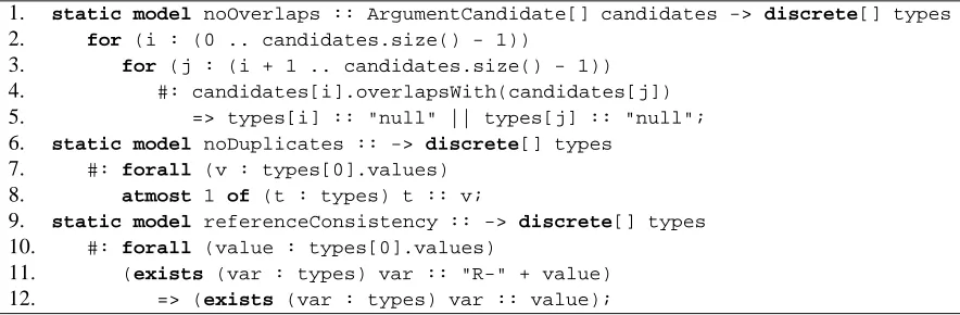
Figure 2: Structural constraints and domain specific expert knowledge encoded as hard constraints are defined here as separate models with no learning components.
1. model SRLProblem :: ArgumentIdentifier ai, ArgumentType at,
2. ArgumentCandidate[] candidates
3. -> boolean[] isArgument, discrete[] types
4. for (i : (0 .. candidates.size() - 1))
5. 100: isArgument[i] <- ai (pertinentData candidates[i]); 6. 1: types[i] <- at (pertinentData candidates[i]); 7. #: ˜isArgument[i] => types[i] :: "null";
8. types[*] <- noOverlaps candidates; 9. types[*] <- noDuplicates ();
10. types[*] <- referenceConsistency ();
Figure 3: The SRL system from Section 2.2. This code captures the decomposition of the inference problem into two learned components and several hard constraints. A wide variety of learning and inference approaches can now be applied over this structure.
declares a structural constraint over every pair of argument candidates that says, “if two constraints overlap, they can’t both have non-nulltype.” The other two models encode knowledge about the global behaviors of the output vari-ables. The model on line 6 says, “each argument type may appear at most once in the sentence,” and the model on line 9 says, “no reference type may appear unless it corresponds to a referent.”
None of these models contain any learned weights. How-ever, they are not considered hard-coded because there are usually multiple valid outputs they might produce for a given input, and LBJ makes no guarantee as to which will be chosen.
Inference: Figure 3 puts all these components together in the global model. By applying the learned models on each argument candidate (as in lines 5 and 6), we construct the objective function in equation (17). The scaling factors appear at the beginning of the lines before the colon and give preference to the decisions of the filter classifier. This results in features of the form described by equations (14) and (15). We also enforce the filter constraint as defined by equations (16) on line 7. Finally, the externally defined constraints are applied to the global model in lines 8-10.
The SRLProblem model takes native Java objects repre-senting candidate SRL arguments as input, defines input and output variables with respect to those objects, and ap-plies the learned models and hard constraints over those variables. Model application is a mechanism through which
the relationships described by one model can be established amongst selected variables in another model. It is accom-plished by binding the inputs and outputs of the applied model to the inputs and outputs (respectively) in the par-ent model (which is SRLProblemin this case). Binding is different than assignment, because no results have been computed. Instead, we are simply declaring that a particular externally defined model’s structure appears in this model.
Lines 5, 6, 8, 9, and 10 of Figure 3 are all examples of model application. They use the left arrow (<-) operator, which binds variables in the manner described above. The model application itself appears to its right, and the newly bound output variables appear to its left. In general, inputs must be bound with inputs and outputs with outputs. The only exception is when the applied model is hard-coded. Since a hard-coded model’s output is already completely determined and cannot be affected by the context in which it is applied, its output variables may be bound with input variables in a parent model. We seepertinentData ap-plied in this way in lines 5 and 6.
3.2. Features and Constraints
The relationships between variables that we have alluded to throughout this paper come in the form of features and constraints. The roles that these two constructs play in a CCM are very similar. Each one simultaneously
• distinguishes a potential property of the variables and
• measures the presence or strength of that property in the variables’ current values.
They are specified as predicates in a first order logic (FOL) syntax in which variables play the role of objects. That syn-tax contains the usual connectives and quantifiers, as well as equality and inequality predicates (:: and!: respec-tively) and quantifiers that can compare the quantities of objects that satisfy a predicate.
3.2.1. Features
To distinguish features from each other, we give them names. These names act as the indexes on features, con-straints, and weight vectors we saw in Section 2. The strength of the feature is the real valued result that is mul-tiplied by the weight with the same name. However, for simplicity, in this paper we will focus on Boolean features, whose strengths can be 0 or 1.
Features’ names and values come from the variables they are functions of, and the structure of the feature functions themselves. As in most programming languages, variables are referred to with identifiers and are used to store interest-ing bits of data. LBJ has Boolean, discrete, and real vari-ables. It also provides dictionaries in which the keys act as separate variable names. Dictionaries can be accessed with either integers or strings inside square brackets (e.g. tags["foo"]) or the selection operator and an identifier (e.g.tags.foo). Both of those syntax examples will refer to the same variable.
Anywhere in the body of a model, a declarative fea-ture statement indicates that the model will include a weight associated with the specified feature. For exam-ple, headWord :: "office"is a feature that evaluates to true if and only if theheadWordvariable takes the value "office". The name of the feature will be its entire lex-ical form, after any interpolation that need be done in the indexes of dictionaries.
3.2.2. Constraints
The same FOL syntax is available for the specification of constraints, except that each constraint statement is pre-fixed with a real-valued literal or a#symbol standing for ∞followed by a colon. This value is theρcorresponding to the constraint in the objective function. It represents the penalty that is incurred iff the constraint is violated.
Constraints tend to make more frequent use of the quanti-fiersforall,exists,atleast,atmost, andexactly. These quantifiers have essentially the same semantics as in LBJ’s prior version, though theexactlyquantifier is new. Its form is:
exactly n of (var:set) sentence
and it is semantically equivalent to
atleast n of (var:set) sentence /\ atmost n of (var:set) sentence
3.2.3. Extensions to First Order Logic
LBJ extends the typical semantics of these logical sentences to allow several unorthodox types of atoms. First (and least ground-breaking),booleanvariables may appear in a fea-ture statement anywhere an atom normally would. They are treated as if they are 0-ary predicates.
Second, discrete variables may appear as atoms. When-ever discrete variables appear as atoms without being com-pared to a value or another variable via the::or!: opera-tors, the feature statement that contains them actually repre-sents many features, one for each set of values in the cross product of the variables in question. Each of these fea-tures will have its own weight in the model. For example, given a discrete variableA∈ {"a1","a2","a3"}and a Boolean variableB, the featureA /\ Brepresents three separate features: A :: "a1" /\ B,A :: "a2" /\ B, andA :: "a3" /\ B.
Third, a dictionary with an index of *(e.g. types[*])
may appear as an atom. When it does, each variable in the dictionary is substituted into the feature in turn, each creat-ing a new feature statement. These new feature statements are subject to the same rules described above depending on whether the substituted variables are Boolean or discrete.4
Thus, it is easy to specify the CCM structure of a multi-class multi-classifier as we saw in Section 3.1. Special provisions must be made to accomodate this behavior with logical op-erators other than conjunction (Cumby and Roth, 2003). LBJ currently does not make those provisions, but the same effects are possible with quantifiers and equality predicates.
New to this version of LBJ is thebooleanvariable, which is an atomic feature. There is also a new operator for ma-nipulating Boolean features (though we only envision it useful when applied tobooleanoutput variables) denoted
ˆ, an example of which appears on line 2 of Figure 1. This operator changes the range of its argument from{0,1}to {−1,1}, thereby making it possible to model linear thresh-old units as described in Section 2.1.1.
4.
Learning and Inference
So far, we have shown how to define the shape and struc-ture of a Constrained Conditional Model using Learning Based Java. The code we have written so far defines that structure and nothing more; it is completely agnostic to both learning and inference. From here, with the help of a sufficiently comprehensive library, the average program-mer should need only select the algorithms of his choice.
For inference in particular, one of the key advantages to im-plementing a model as a CCM is that it is always possible to fall back on Integer Linear Programming (ILP) to solve the inference problem. Since CCMs keep their objective
4
1. for (i : (1 .. vars.size()-1))
2. newScores <- double[];
3. for (current : vars[i].values)
4. for (prev : vars[i-1].values)
5. s = scores[prev] + problem.score {vars[i] = current; vars[i-1] = prev};
6. if s > newScores[current] then
7. newScores[current] = s;
8. predictions[i][current] = prev;
9. scores = newScores;
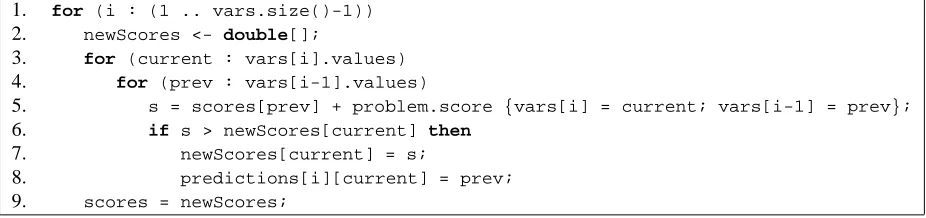
Figure 4: A code sample from an LBJ implementation of the Viterbi algorithm. On line 5, the model returns the score of a partial assignment to the output variables. This is a computational building block for many inference algorithms.
functions linear and their features and constraints in a logic language, they can be automatically translated to ILP opti-mization problems. While ILP is intractable in general, it has been successful in practice on a variety of tasks, even when incorporating long range constraints (Punyakanok et al., 2008; Denis and Baldridge, 2007; Martins et al., 2009). However, if the task at hand demands a more problem spe-cific approach, LBJ can help.
4.1. Inference
Inference in LBJ is often as simple as naming the algorithm and the output variables to apply it to. This is the case in the following code, where we see the implementation for an approximate solution to our running SRL example.
1.solver SRLInference :: SRLProblem problem
2. Greedy.solve problem.isArgument[*]; 3. ILP.solve problem.types[*];
First it applies a greedy algorithm to theisArgument vari-ables, literally executing the argmax in equation (2) over each output variable individually. The resulting assign-ments for these variables are now fixed, making the job of the next inference algorithm called a little easier.
However, it is often the case that the structure of the prob-lem indicates a particularly appropriate algorithm that was not anticipated in the LBJ library. For example, the HMM (Section 2.1.3.) is efficiently solved by Viterbi. Of course, LBJ has a Viterbi implementation, and Figure 4 shows a snippet from it. But from this snippet, we can see an im-portant bit of LBJ’s syntactic sugar that makes writing in-ference algorithms easier. On line 5, the model is queried for the score of a partial assignment to the output variables.
A partial assignment score query can be performed over any subset of output variables. The result is the usual eval-uation of eqeval-uation (1), except every feature and constraint function whose evaluation depends on a variable outside the partial assignment is assumed to return 0. In the context of a CCM specified in LBJ, the programmer also has access to the names of the variables and can thereby pick out their structure to guide his inference procedure. Thus, a host of ad hoc inference implementations become possible.
4.2. Learning
Like inference algorithms, learning algorithms can be im-plemented externally and linked to LBJ. However, LBJ also provides several facilities that make it easier to write
learn-ing algorithms. First, output variables can contain both la-bels and predicted values. This comes in handy when writ-ing a supervised learnwrit-ing algorithm. Second, a model can act as a feature extractor that returns a feature vector. Fea-tures can be extracted using either the labels or the current predicted values in the output variables. Third, the lan-guage contains syntactic sugar that lets models be treated as weight vectors for the purpose of performing linear al-gebra with respect to feature vectors. Combined with the ability to query for the scores of partial assignments as de-scribed above, the programmer has the necessary tools for building custom learning solutions quickly.
5.
Data Driven Compilation
The biggest advantage to developing a machine learning framework as a stand-alone language as opposed to a li-brary for an existing general purpose langauge is that it opens many opportunities for automatically improving the efficiency of the code based on high level analyses. LBJ ex-ploits these analyses with a unique twist, since much of the information necessary to generate the final program code is only available in the training data. Thus, we say that an LBJ compiler performs data-driven compilation. Feature extraction is perhaps the biggest beneficiary of data driven compilation.
In most NLP systems, a lexicon associating each feature with a unique integer index is built from the training data. These integers are used to index the weight vector, which is implemented simply as an array. Many NLP systems create a separate entry in the lexicon’s hash table for every unique feature. Since many NLP systems have millions of fea-tures, the resulting code will use a lot of memory and will be slowed by the abundance of accesses to the hash table.
Lexicons created by LBJ, on the other hand, only store in-dexes associated with the discrete values each input and output variable are observed to take. For any discrete vari-able that can take one ofk possible values, each value is associated with a number between 0 andk−1 inclusive in the lexicon. Then they organize the feature index space so that features that have the same topology while merely comparing their constituent variables with different values are grouped together. This will happen frequently, since features that use discrete variables and dictionaries as atoms are quite common.
com-pute recursively, as functions of the indexes of their subex-pressions, the indexes of the larger formulas that are active given a variable assignment. These indexing functions get their behavior from the connectives used in the feature for-mulae. For example, if a featuref is a conjunction of two formulae f1 andf2, its active indexes will take the form I(f) =kf2I(f1) +I(f2) + Ωf, wherekf2 is the number of features in the same group asf that differ only by value comparisons made in f2, andΩf is an offset that ensures the index space off begins immediately after the previous feature’s index space ended.
Disjunction complicates things a little, since many features in a group of disjunctive features can be active simulta-neously. For example, when the features A :: "foo" \/ B :: "bar"andA :: "foo" \/ B :: "baz"are grouped together, both will be active if the variable A is set to"foo". The result is that sets of active indexes are returned up the recursion, and the parent formula’s index computation loops over the cross product of these sets to compute its indexes.
The constants in the index formulae can be computed at compile time, after an initial pass over the data, but before training begins. The end result is a lexicon orders of magni-tude smaller and generated code that performs swift feature extraction, making any algorithm implemented in the lan-guage more efficient.
6.
Conclusion
In this paper we described a modeling formalism for mul-tivariate models (CCM) and showed that it is appropriate for a wide variety of NLP tasks. We then developed a pro-gramming language (LBJ) for specifying the models and peforming learning and inference over them. Finally, we showed that the feature extraction syntax of the language can be compiled to code efficient in both space and time. Using LBJ, we believe NLP systems that use learning and inference can be developed rapidly, since the developer will spend most of his time thinking about the modeling of his problem from a high level.
Acknowledgements
The authors would like to thank Ming-Wei Chang, James Clarke, and Vivek Srikumar for many insightful conversa-tions. This work was supported by NSF grant NSF SoD-HCER-0613885.
7.
References
R. Barzilay and M. Lapata. 2006. Aggregation via Set Par-titioning for Natural Language Generation. In Proc. of HLT/NAACL.
E. Bengtson and D. Roth. 2008. Understanding the Value of Features for Coreference Resolution. In Proc. of EMNLP.
A. Carlson, C. Cumby, J. Rosen, and D. Roth. 1999. The SNoW Learning Architecture. Technical report, UIUC Computer Science Department.
M. Chang, L. Ratinov, N. Rizzolo, and D. Roth. 2008. Learning and Inference with Constraints. In Proc. of AAAI.
M. Collins. 2002. Discriminative Training Methods for Hidden Markov Models: Theory and Experiments with Perceptron Algorithms. In Proc. of EMNLP.
K. Crammer and Y. Singer. 2003. Ultraconservative On-line Algorithms for Multiclass Problems. Journal of Ma-chine Learning Research.
C. Cumby and D. Roth. 2003. Feature Extraction Lan-guages for Propositionalized Relational Learning. In IJ-CAI Workshop on Learning Statistical Models from Re-lational Data.
H. Cunningham, D. Maynard, K. Bontcheva, and V. Tablan. 2002. GATE: A Framework and Graphical Development Environment for Robust NLP Tools and Applications. In Proc. of ACL.
P. Denis and J. Baldridge. 2007. Joint Determination of Anaphoricity and Coreference Resolution using Integer Programming. In Proc. of NAACL.
T. G¨otz and O. Suhre. 2004. Design and Implementation of the UIMA Common Analysis System. IBM Systems Journal.
N. Littlestone. 1988. Learning Quickly When Irrelevant Attributes Abound: A New Linear-threshold Algorithm. Machine Learning.
E. Loper and S. Bird. 2002. NLTK: the Natural Language Toolkit. In Proceedings of the ACL-02 Workshop on Ef-fective Tools and Methodologies for Teaching Natural Language Processing and Computational Linguistics. T. Marciniak and M. Strube. 2005. Beyond the Pipeline:
Discrete Optimization in NLP. In Proc. of CoNLL. Andre Martins, Noah Smith, and Eric Xing. 2009.
Con-cise Integer Linear Programming Formulations for De-pendency Parsing. In Proc. of ACL.
A. McCallum, K. Schultz, and S. Singh. 2009. FACTO-RIE: Probabilistic Programming via Imperatively De-fined Factor Graphs. In NIPS.
V. Punyakanok, D. Roth, W. Yih, and D. Zimak. 2005. Learning and Inference over Constrained Output. In Proc. of IJCAI.
V. Punyakanok, D. Roth, and W. Yih. 2008. The Impor-tance of Syntactic Parsing and Inference in Semantic Role Labeling. Computational Linguistics.
L. R. Rabiner. 1989. A Tutorial on Hidden Markov Models and Selected Applications in Speech Recognition. Pro-ceedings of the IEEE.
L. Ratinov and D. Roth. 2009. Design Challenges and Mis-conceptions in Named Entity Recognition. In Proc. of CoNLL.
M. Richardson and P. Domingos. 2006. Markov Logic Networks. Machine Learning Journal.
N. Rizzolo and D. Roth. 2007. Modeling Discriminative Global Inference. In Proc. of ICSC.
F. Rosenblatt. 1958. The Perceptron: A Probabilistic Model for Information Storage and Organization in the Brain. Psych. Rev. (Reprinted inNeurocomputing(MIT Press, 1988).).
D. Roth. 1999. Learning in Natural Language. In Proc. of IJCAI.