Omnitrans International BV, University of Twente
X-Stream in MaDAM
Omnitrans International BV, University of Twente
X-Stream in MaDAM
New junction modelling in
macroscopic dynamic traffic
assignment models
Documentation page
Client(s) Omnitrans International BV., University of Twente
Title report X-Stream in MaDAM
New junction modelling in macroscopic dynamic traffic assignment models
Author M.P. Schilpzand
Date of publication 27/06/08
Mentors Ir F. Brandt (Omnitrans International), dr. G. Still (University of Twente) Project Definition Graduation Thesis
Acknowledgements
Thinking that the acknowledgements would be the easiest and most joyful chapter of this thesis to write, I find it fascinating that I am a bit lost at what to write here. There are of course those that deserve my gratitude and credit for the help they have given me in the year it took me to write this thesis, and they will get it here. However I know that at least as important for me is the atmosphere at my workplace, the joy I have in doing my research and the relaxation at home. Therefore I would like to begin with thanking all of you guys at work, at volleyball and in my free time who made me laugh and relax. Above all my deepest gratitude goes to Aniek without whom I couldn’t have had this level of happiness. Which, for me, is the best basis for good research and a good thesis!
Now I would like to give credit to those people who deserve it. My two mentors, Feike Brandt and Georg Still. Feike, thank you for giving me the freedom to make my own mistakes and learn from them. I would also like to thank you for being optimistic but never hesitant to ask the tough questions to make my research better, and for making time (almost) every Monday in your busy schedule. As for Georg, all throughout the year I was thinking of how special it was to have a mentor who was sick most of the time and still had time to meet me once per month and had suggestions and critics when due. So Georg, thank you most of all for the time you gave me in spite of your sickness.
My colleagues who, aside from the joyful time, also always seemed to have time for me whenever I needed an answer or wanted to brainstorm. Especially Edwin, thank you for never hesitating to answer me. Whether there was something I didn’t understand in the code, in MaDAM, in OmniTRANS or just had a general question. Also Mark thanks for getting me in touch with Omnitrans.
Finally a “thank you” to my family and again Aniek who, despite of the difficulty of my study, never stopped showing fascination in my work and who always tried to comprehend when I was speaking the foreign language of mathematics again.
Summary
Samenvatting
Macroscopisch Dynamisch Verkeer Toedeling (MDVT) modellen worden veel gebruikt bij het voorspellen van de impact van voorgestelde verkeersaanpassingen. De meeste MDVT modellen zijn ontwikkeld voor het hoofdwegennet. Recentelijk worden ze echter ook veel voor het onderliggend wegennet gebruikt. Een groot verschil tussen het hoofdwegennet en het onderliggend wegennet is de aanwezigheid van kruispunten. Dit verslag beschrijft hoe de effecten van kruispunten meegenomen kunnen worden in MDVT modellen.
Contents Page
1 Introduction 1
1.1 Research goals 1
1.2 Structure of the thesis 2
2 Function of a MDTA model 3
2.1 Macroscopic dynamic traffic assignment models explained 3
2.2 Quantities explained 3
2.2.1 Fundamental diagram 4
2.3 Conservation Equation 7
2.4 Velocity dynamics 8
2.4.1 Continuum model 8
2.4.2 Discrete model 11
2.4.3 Different sound speed of traffic functions 14
2.5 The Link Transmission Model 16
3 Junction Modelling 17
3.1 Junction modelling explained 17
3.2 Basic approach 18
3.3 Current model 18
3.3.1 Explanation of the currently used model 18
3.3.2 Known problems 20
3.3.3 Improvements 23
4 The link between junction modelling and a macroscopic dynamic traffic
assignment model 24
4.1 Important variables of junctions and MDTA 24
4.1.1 Input variables for junctions 24
4.1.2 Output variables of junctions 25
4.1.3 Variables which are both input and output for macroscopic dynamic traffic
assignment models 26
4.1.4 Input variables of macroscopic dynamic traffic assignment models 27 4.1.5 Output variables of macroscopic dynamic traffic assignment models 27 4.2 Exchange of variables between MaDAM and Junction Modelling 28
4.2.1 From MaDAM to Junction Modelling 28
4.2.2 From Junction Modelling to MaDAM 28
4.3 (In)dependency of JM with respect to MaDAM 28
5 Subsequent questions 29
5.1 Junctions in other MDTA models 29
6 Main question and the future 31
7 Explanation of the new algorithm 33
7.1 Principle of the new model 33
7.1.1 Basic approach 33
7.1.2 Handling known problems and improvements 33
7.1.3 Procedure 33
7.1.4 Remarks 34
7.2 Schematics of the algorithm 46
7.3 Calibration and validation 47
7.3.1 Propagation model with new anticipation term 47
7.3.2 Speed and capacity of junctions 48
7.3.3 Complete junction effects 48
8 Conclusions and recommendations 49
8.1 The effects of junctions in macroscopic dynamic traffic assignment models 49
8.1.1 Conclusions 49
8.1.2 Recommendations 49
8.2 The development of a new algorithm 50
8.2.1 Conclusions 50
8.2.2 Recommendations 50
9 References 51
Page 1
1
Introduction
The concept of transportation has been around ever since men settled down and founded homes. In the beginning little was going on. However, since the twentieth century, the transportation sector has seen a dramatic increase in number of vehicles and turnover. As there are literally billions of euros spent in traffic, this sector has become more and more important which resulted in the increase of importance of traffic models. A set of these models are the macroscopic dynamic traffic assignment (MDTA) models. These models were developed somewhere halfway the twentieth century in order to have scientific methods for attacking the problem of organizing road traffic so that the full benefits of the increased mobility can be enjoyed at the lowest cost in human life and capital [LW55]. These models were originally developed for use on highways. With the ascending of the computer however they were soon used on suburban roads and recently even on urban roads. A large difference between highways and (sub)urban roads which has to be dealt with, is the presence of junctions. Macro dynamic traffic assignment models should therefore take into account the effects of junctions on traffic flows. This leads to the first goal of this thesis; to formulate a global theory of how to take into account the effects of junctions in macroscopic dynamic traffic assignment models. The second goal of this research is the development of an algorithm which deals with junctions in MaDAM and can be implemented in its code. MaDAM stands for Macroscopic Dynamic Assignment Model and is the MDTA used and developed by Omnitrans International.
1.1
Research goals
The first goal of this thesis can be formulated as a question: How can the effects of junctions be taken into account in a macroscopic dynamic traffic assignment model? The second goal, the development of an algorithm which deals with junctions in MaDAM, is essentially nothing more than the first goal applied to the MDTA of OmniTRANS. The questions leading to answering the main question and to the development of the algorithm are therefore sometimes global and sometimes more specific for development. It is of essential importance for answering the main goal that it is clear what a MDTA model is and what the function is of a junction. This leads to the first two preliminary questions: What is the function of a macroscopic dynamic traffic assignment model? And: What is the function of junction modelling? When these two questions are answered the logical next step is the link between the two models: What are the important variables of a macroscopic dynamic traffic assignment model and junction modelling? Closely connected to this last question is one leading to the second goal: Which variables are being exchanged between MaDAM and Junction Modelling? Also important for the development of an algorithm is: What is the (in)dependency of Junction Modelling with respect to MaDAM?
Page 2
This leads to two more questions: In what way do other MDTA models deal with junctions? And: Can a static (junction) model deal with its umbrella dynamic model? Because of the planning that more macro dynamic traffic assignment models could be implemented in OmniTRANS, it is also important to know what the future will bring: How can a macroscopic dynamic traffic assignment model deal with junctions in the future?
1.2
Structure of the thesis
Page 3
2
Function of a MDTA model
This chapter treats the basics of macroscopic dynamic traffic assignment models. Its function is explained here as well as the mathematics behind the model. Most elaborately explained is the model used in MaDAM at this moment. This is a model based on an MDTA model developed by Messmer and Papageorgiou [MP90], which itself is based on an MDTA made by Payne [Pay71]. Also mentioned is the link transmission model, a new MDTA model developed by Ypperman [Ype06], which could be interesting if a new MDTA model is implemented next to MaDAM.
2.1
Macroscopic dynamic traffic assignment models explained
One way of modelling traffic is by means of macroscopic dynamic traffic assignment models. Macroscopic models all describe the flow of traffic, the traffic streams. Traffic is therefore not viewed as cars driving on a road (as is with microscopic models) but more as some substance flowing on the roads. There are two different macroscopic models, first order and higher order models. The most famous first order model is the LWR-model [LW55], explained in paragraph 2.3. First-order models however have some shortcomings. Harold Payne [Pay71] was one of the first to recognize this and developed a higher-order model, explained in paragraph 2.4. Firstly however, in paragraph 2.2, the quantities used as well as the fundamental diagram are explained.
2.2
Quantities explained
Basic quantities
The three most important quantities in a macro-dynamic propagation model are flow, concentration (or density) and speed (or velocity). The flow is defined as follows: q
n
So the flow is the average number of vehicles passing a certain point of the road during some time period. The common unit of flow is: number of vehicles per hour. The concentration on a piece of road is defined as: k
dt
time taken by vehicle to cross a slice of road length of the slice of road
Page 4
To make things more clear imagine some road with two lines a distance apart. Now measure all the times taken by the vehicles to cross this slice of road over a moderate time interval
dx
( )
dt.
τ This interval has to be long enough for many vehicles to pass. All the times taken by the vehicles to cross the slice of road added and divided by the time interval
(
∑
dt τ)
gives the average number of cars on that slice of road. When this average is divided by the length of the slice, it gives the number of vehicles per unit length of road. The common unit of concentration is: number of vehicles per kilometre. The velocity vis defined as:1
q dx
v k
dt n
= =
∑
(2.2.3)This is the average of vehicle speeds weighted according to the time they remain on the slice of road.
2.2.1 Fundamental diagram
For a relation between two of the quantities a so-called fundamental diagram is used. In this diagram two of the three quantities are depicted. Because of the relationship
,
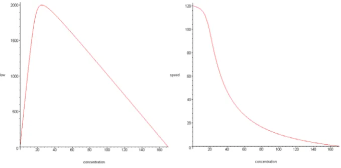
q= ⋅k v diagrams with other combinations of quantities can be made. Several types of fundamental diagrams are available. As an example a flow-concentration curve and a speed-concentration curve can be seen in Figure 1.
Figure 1: Flow-concentration curve and speed-concentration curve
These curves are based on the Van Aerde car following model [RC02]. This model depends on four parameters, namely:
. Roadway free speed, the maximum speed of the road,
. Speed at capacity, the speed with maximum flow,
. Capacity,
Page 5
Equation (2.2.4) gives the formula for a so-called “fundamental diagram”:
2
The deduction of the formulas for are done in the following section. The term headway is the distance between the front bumpers of two successive vehicles. The relation between headway and concentration is
, concentration and the speed is:
2
Using this relation and the fact that k v⋅ =q,enables one to calculate the relation between the flow and the speed:
2
Explanation of parameters in the fundamental diagram
For equation (2.2.6) two conditions exist. The first condition is that the maximum flow rate occurs at the speed-at-capacity when the derivative of the flow rate with respect to speed is equal to zero. The second condition is that at jam concentration the traffic speed is equal to zero.
Page 6
From the first condition follows:
(
)
Simplifying this gives:
2
Which in turn can be written as:
(
) (
)
By setting the speed equal to zero in (2.2.5), the second condition gives:
2 1 2
Solving equation (2.2.10) for c1gives:
2
Combining formulas (2.2.9) and (2.2.11) gives a new equation for independent of
With this formula for is also fixed for given free-speed, speed-at-capacity and concentration-at-capacity. For the calculation of equation
,
2 1
c c
3
Page 7
So the relation between two of the units of speed, concentration and flow depends, as mentioned above, on free-speed, the speed-at-capacity, the capacity and the jam concentration.
2.3
Conservation Equation
The LWR-model of Lighthill, Whitham and Richards describes how slight changes in flow are propagated back through the stream of vehicles along ‘kinematic waves’. One of the main equations in this model is the conservation equation, a partial differential equation that describes the conservative transport of some kind of quantity. In this paragraph, the conservation equation for traffic streams is deduced from a general form for fluids. The general form of the conservation equation is [Vel93]:
( )
0density of the fluid velocity of the fluid
n
In traffic the relation between density, velocity and flow is:
q=kv (2.3.2)
Combining (2.3.1) with (2.3.2) and noting that the dimension of space in this equation is equal to 1 gives:
Page 8
2.4
Velocity dynamics
2.4.1 Continuum model Conservation equation
The principle of the theory of Payne is to combine the kinematics of Lighthill and Whitham with a car-following model and make this model discrete [Pay71]. The quantities
are used again and are related by the identity:
, and
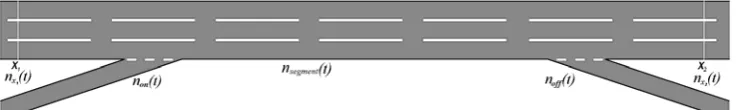
in any time-space segment. To derive a discrete model of a segment between locations
1and
x x over the time interval observe that for the number of cars in this segment the following holds:
,
segment segment x x x x
on on off off
number of vehicles on the segment at time
total number of vehicles generated on point at time total number of vehicles generated on point at time total number of vehi
segment
cles generated on on-ramp at time total number of vehicles generated on off-ramp at time off
t
n t = t
Figure 2: Conservation of vehicles
Now define the flow, concentration and on- and off-ramp frequencies as follows:
Page 9
Using the definitions of (2.4.3), equation (2.4.2) can be rewritten to:
(
) (
)
(
) (
)
(
)
Equation (2.4.5) is a generalized form of the conservation equation (2.3.3). Where (2.3.3) stated that no vehicles could turn up out of nowhere or disappear into nothingness, (2.4.5) says that there could be a change in the number of vehicles due to on-ramps and/or off-ramps.
Dynamic equation
Next to the expanded conservation equation a car-following model is reviewed. Suppose that at some moment the position of a vehicle is given as:
( )
With the vehicle position known, the spacing between vehicles is next examined. This spacing can be approximated by the reciprocal of the density:
( )
( )
( )
The density in this formula depends on space and time. The space
( )
x is set to the place of vehicle A more accurate representation is the density at a location midway between the vehicles. This location can be approximated by taking the current location and adding halfthe headway at the current location:
.
Page 10
To include the reaction time observe that the vehicle at time is approximately at position
,
T t+T
( )
,x T v x t+ ⋅ assuming that the velocity doesn’t change in time-interval
[
t t T, +]
,this assumption can be made because the reaction time is very small compared to other time-scales on the highway. Expanding formula (2.4.9) gives:(
)
(
( )
, ,)
n
y t+T →v x T v x t+ ⋅ t+T (2.4.10)
Because the reaction time is small, the right-hand side of expression (2.4.10) can be expanded using Taylor’s series in T:
(
)
( )
( )
(
(
( )
)
)
( ) ( )
(
)
( )
Using the substitution of the steady-state velocity for the vehicle speed suggested by Gazis [GHR61] and deleting higher order terms, one gets:
( ) ( ) ( )
, , , 1(
( )
, e(
( )
(
,)
steady-state velocity, depending on the concentration eV k x t =
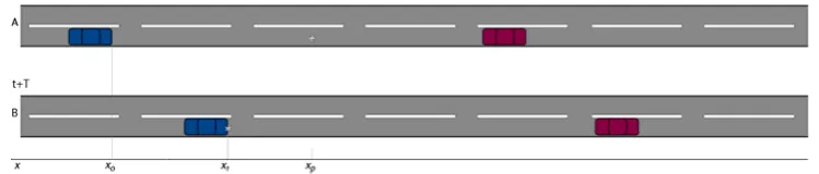
The steady-state velocity can be obtained by means of the fundamental diagram as shown in Figure 1. The steady-state velocity depends on the concentration at a certain point in time and space. This point can be explained using Figure 3.
Figure 3: Steady-state velocity explained
In this figure two roads are depicted. Road A can be seen as a picture taken from above at time where the left car is vehicle and the front of this vehicle is said to be at position t, n
. 0
Page 11
The vehicle speed at time t T+ therefore depends on the headway between cars and n 1
n− at time As seen before in equationt. (2.4.8), the headway can be approximated by
( )
, .1
2k x t This point in time and space is depicted by the white plus-sign in Figure 3. Using these variables for time and space, equation (2.4.12) can be rewritten as:
( ) ( ) ( )
( )
( )
In equation (2.4.13) it can be seen that Payne stated that the momentum of the fluid, the derivative of speed to time, has three different aspects: a convection term describing how the speed changes due to the arrival and departure of vehicles, a relaxation term describing how vehicles adept their speed according to the fundamental diagram and an anticipation term describing how vehicles react to the concentration conditions downstream of the road. This anticipation term can be made more general by defining a model-dependant sound speed of traffic c k
( )
,the dynamic equation then becomes:( ) ( ) ( )
( ) ( )
( )
2.4.2 Discrete model
For modelling purposes the speed, concentration and flow given at points are not as useful as speed on intervals and concentration and flow on segments. Equation (2.4.14) should therefore be made discrete. First the important quantities are defined on segments (speed and capacity) or time steps (flow):
Page 12
average number of vehicles passing point between and mean speed on section between points and at time mean number of vehicles on section between points and
q x t t x t t
For the derivative of the speed to space, Payne uses a backward difference formula, for the derivative of the concentration to space he uses a forward difference and for the derivative of the speed to time Payne again uses a forward difference approximation:
( )
(
)
(
)
For the derivative of concentration to time and of flow to space, similar difference approximations can be used:
( )
(
) (
)
To make the equations a little easier to understand, define the following discrete variables:
(
)
So qnjis defined as the flow of cars passing a point, located jtimes the segment length from x0,in the time interval between n−1times the time step and times the time step. The speed is defined as the average speed on a slice of road starting
Page 13
Conservation equation
On segments with on-ramps traffic has to merge and on segments with off-ramps traffic has to diverge. Because both merging and diverging flows are special cases of fluid streams they are not considered here and instead of the more general form, equation (2.3.3), which considers no on- or off-ramps, will be made discrete:
( )
,( )
,The derivatives of flow and concentration are replaced by section flow and section concentration, defined in equation (2.4.17):
(
, ;) (
, ;)
(
; ,) (
; ,)
section length (equal for all section)
x
Δ =
Using the variables from equation (2.4.18), the conservation equation then becomes:
1
Rewriting this equation to a formula of the concentration on the j'thsection at time 1
The relation given in equation (2.4.1) still holds for sections and is rewritten as:
n n
j j
q =k ⋅v (2.4.23)
The concentration, flow and speed are all per lane, for modelling purposes however it is more natural to have a flow on a road than a flow per lane. The flow per lane is therefore multiplied by the number of lanes to return a flow for the total road.
At the start of this section it was assumed there would be no on- or off-ramps. When a segment actually has an on-ramp, traffic has to merge which results in an extra term in the dynamic equation. When a segment has an off-ramp, traffic has to diverge which results in dividing the streams over different roads. Both cases however are specially modelled and fall outside of the scope of this thesis.
Dynamic equation
Taking again the more general form of the dynamic equation (2.4.14) which is slightly rewritten:
Page 14
section length (equal for all section)
x
Δ =
Using the variables from equation (2.4.18), the dynamic equation then becomes:
( )
2( )
Rewriting this equation to a formula of the speed on the j'thsection at time n+1gives:
(
)
(
( )
)
2( )
So the speed a time step further equals the speed at that section at this time adjusted by three terms, the convection, relaxation and anticipation term.
Equations (2.4.22), (2.4.23) and (2.4.27) together give an iterative scheme for the calculation of which are used in computer packages simulating macroscopic dynamic traffic assignment models.
, and
n n n
j j j
k q v
2.4.3 Different sound speed of traffic functions
For the function c k
( )
there are several options [Mae06]. In the next paragraphs three of these options are elaborated. For a better understanding of the different functions, a new study has to be done, as this is too expansive for the current thesis. The three functions treated are those of Payne [Pay71], Zhang [Zha98] and Messmer & Papageorgiou [MP90].Payne
Page 15
The whole dynamic equation now becomes:
(
)
(
( )
)
( )
1For the derivative of the fundamental diagram speed to the density d Ve
( )
knj dk⎛ ⎞
⎜ ⎟
⎝ ⎠there are
two options. One is really calculating the derivative when the equations of the fundamental diagram are given. Problem with this option is that calculating the derivative can be an elaborate job and therefore can cost a lot of time, especially when the fundamental diagram of Van Aerde is used. The other option is estimating the derivative by means of a forward difference formula again. The anticipation term is than changed as follows:
The sound speed of traffic function suggested by Zhang only depends on the derivative of the fundamental diagram speed to the concentration and the concentration itself:
( )
n e( )
njThe whole dynamic equation now becomes:
(
)
(
( )
)
( )
As described above there are two options for the derivative of the fundamental diagram speed to the density again. The first option being the real calculation of the derivative, which is cumbersome. The second option being the estimation of the derivative via a forward difference formula again. The anticipation term is than changed as follows:
Page 16
Messmer & Papageorgiou
The sound speed of traffic function suggested by Messmer & Papageorgiou is the simplest of the three options. Instead of dependency on the derivative of the fundamental diagram speed, this function depends on the concentration, the reaction time and two global parameters:
The whole dynamic equation now becomes:
(
)
(
( )
)
(
)
1In Messmer & Papageorgiou’s model, the values of the parameters are given and are the following:
At this moment MaDAM uses the function of Messmer & Papageorgiou. As mentioned before however, this choice is open to debate and further research is needed.
2.5
The Link Transmission Model
Page 17
3
Junction Modelling
In this chapter the function of junction modelling is explained. The effects of junctions on traffic flows come up for discussion as well as two different ways in which junctions can be modelled. On the basics of the currently used model some errors which can occur are treated and improvements are discussed.
3.1
Junction modelling explained
On highways traffic can be modelled comparatively easy with fluid models. Models for traffic flows just need to take into account the presence of bottlenecks, on- and off-ramps and some special cases as merging and diverging lanes.
In urban areas the models will no longer be easy, as a new type of node will come in perspective: the cross-node. On this node at least two flows of traffic will meet, interact and leave again. The interaction can occur in a lot of different ways. Part of one of the flows just needs to cross the other flow, another part needs to diverge one way or another. To make it even more complicated, the cross-node can have specific requirements such as traffic lights, roundabout or priority roads.
Now a junction has to take into account two different effects:
. Interaction between two (or more) traffic streams. For example, one stream going from south to north has to cross a stream going from the west to the east. Another interaction could be the merge of a stream from south to north with a stream from west to north.
. Extra limitations. Some junctions have specific conditions which have to be considered. Traffic lights for example block a flow for some time and let it flow for some other time. This can be seen as a bottleneck with a capacity of zero for certain (set) times and maximum capacity for the other times. Another condition could be a stop sign on a junction. This creates extra delay even when the other flow would be very small. The last example is the crossing of pedestrians with traffic lights on a road. Again this can be seen as the bottleneck from the first example. This junction however doesn’t have any interaction between traffic streams.
Page 18
3.2
Basic approach
There are two different ways of modelling junctions in macro-dynamic models.
. The average method in which the characteristics of a junction are calculated beforehand, added to the total travel time in case of a delay or added to the density of the road in case of a queue.
. A more embedded model in which the junction is explicitly evaluated at the step the dynamic model is currently in. When possible a traffic stream then flows over the junction.
Both ways have their advantages and their disadvantages. The first method has the advantage of being simple to implement. The junctions don’t have to be simulated during every time-step of the macro-dynamic model but instead the characteristics can be computed beforehand and these characteristics can be used during the time-steps. With this approach the junction modelling is also fast, again because of the computation beforehand instead of simulating the junction every time-step. A drawback of the first method is the possible occurrence of errors. In section 3.3.2 known problems of the currently used method, based on the first approach, are reviewed. The possible advantage of the second method is the accuracy. Every time-step new intensities can occur on all directions, therefore the capacity and delay for different directions on junctions change with every time-step (see the section Changes of intensities over time for a more detailed explanation). Also the forming of queues can be more pessimistic in real life than in an averaged model (see the section Occurrence of a queue for a more detailed explanation). With an explicit simulation of junctions the queues are formed more natural. A disadvantage of the second method is the length of the simulation. When junctions have to be simulated every time-step and the program also needs to know at what time-step the process is to simulate correct green times, more simulation time will be needed compared to the first method. A special point of explicitly simulating the characteristics of a junction is some series of signalised intersections. When properly modelled, series of signalised junctions can show the effect of a platoon. All junctions in these series however, have to be modelled very precisely which is computationally intensive.
3.3
Current model
3.3.1 Explanation of the currently used model
The model currently used to take into account the effects of intersections on traffic streams has three variables which have to be transferred from the junction model to the propagation model. These variables are:
. Delay: The amount of time a vehicle needs for deceleration, crossing and acceleration
. Capacity: The maximum number of vehicles which can cross the intersection in a given time, typically one hour
Page 19
Of these three the capacity can be transferred directly to the propagation model, the other two have to be rewritten in variables known by the propagation model. Variables of junctions and macroscopic dynamic traffic assignment models are further explained in section 4.1.
Delay
In the current model the junction is calculated once in the beginning to get the correct values i.e. the capacity of the junction, the delay for the different directions and green-times when the junction is signalised. In every time-step the traffic streams for turns on junctions are now viewed, the delay is added and the speed adjusted as explained in Example 1. When the inflow is higher than the capacity of that turn on the junction a queue is formed. The adding of the delay is done by means of adjusting the speed on the segment before the junction such that the time to ride over the segment is the same as the time it took normally with the delay added to this.
Example 1:
Suppose the last segment before a junction has a length of 200 meters, the speed calculated is 36 km/h (or 10 m/s) and the delay is 30 seconds. Normally it would take 20 seconds to cross this segment (200/10), with the added delay it takes 50 seconds, so the speed is adjusted to 14.4 km/h (or 4 m/s).
Queue
Next to the speed adjustments a queue could be formed. This happens when the flow of a specific turn is higher than the capacity of that turn. When there are multiple lanes on a junction, the appropriate lane will first get a queue. The forming of a queue is done by means of a recursive formula:
(
)
number of cars in queue on lane after timesteps inflow on the segment after timesteps
Page 20
For the calculation of the length of the queue, the number of cars in the queue is divided by the maximum concentration for that lane. The maximum concentration is only reached when all the cars are in a queue. The maximum concentration is therefore the number of cars in a queue with a length of one kilometre.
Example 2:
Suppose the last segment for a junction has two lanes, one lane for a left turn and a combined straight and right turn. The fractions of traffic for a left, a straight and a right turn are respectively a quarter, a half and a quarter. Total inflow is 2000, outflow on the left lane is 200, on the combined lane it is 300. Number of cars already in queue are 2 for the left turn and 6 for the combined lane. The length of the time-step is 12 seconds and the maximum concentration is 180. For the combined lane the number of cars in the queue are:
The length of this queue is approximately 56 metres. For the left turn only the number of cars in the queue are:
The length of this queue is approximately 17 metres.
If the inflow remains too high, the queue could spill back on the segment before the last segment. When this happens the queue will grow even faster because now also streams for other turns are in the queue.
3.3.2 Known problems
Two of the main problems of the currently used model for junctions are changes of intensities over time and a too optimistic occurrence of a queue i.e. the queue in the model is not as long as it could be in reality.
Changes of intensities over time
Page 21
Example 3:
Figure 4: Long road with intersection at the end
Suppose there is a road as depicted in Figure 4, where there is only traffic from points 1 to 3 and 2 to 4 the distance from 1 to 3 is 100 kilometre and one kilometre before point 3 there is a crossing with cars from 2 to 4. When there is a lot of traffic from 1 to 3, a static assignment returns a large intensity on the road from one to three, which results in a large delay for traffic from 2 to 4 on the junction, regardless of the fact whether the traffic from point 1 has already reached the junction.
Occurrence of a queue
Page 22
Example 4:
Assume a junction where there are two lanes for a road from some direction, both lanes are 50 meters long. The cycle-time of the signal is 120 seconds of which lane 1 gets 40 seconds, lane 2 gets 60 seconds and some other directions get 20 seconds. Every 6 seconds one car arrives for lane 1 and every 4 seconds one car arrives for lane 2. So direction 1 has a flow of 600 cars per hour and direction 2 has a flow of 900.
Currently used model
When the traffic lights are green, every two seconds one car can leave. This gives a capacity of 600 for direction 1 and 900 for direction 2. Because the capacity and flow are equal no queue will form in the currently used model.
Real life
When a length of the lanes of 50 meters and an average length of 5 meters per car are assumed however, the following table shows a queue will form. The values after 1, 2 and 3 cycle-times (120, 240 and 360 seconds) can be compared best to see this: after 1 cycle a queue of 9 cars is formed, after 2 cycles the queue is 19 vehicles long and after 3 cycles 22.
Seconds Queue on the road Cars on lane 1 Cars on lane 2
0 0 0 0
20 0 0 5
40 0 0 10
60 0 3 5
80 0 7 0
100 1 10 0
120 9 10 0
140 2 6 10
160 10 0 10
180 1 7 10
200 3 10 4
220 11 10 0
240 19 10 0
260 8 10 10
280 16 0 10
300 7 7 10
320 6 10 7
340 14 10 0
Page 23
3.3.3 Improvements
The method currently used for the modelling of junctions in the macro-dynamic propagation model has at least two points of improvements. The propagation of traffic over the junction and the existence of special bottlenecks as open bridges and railway crossings.
Propagation
Because the method used for the modelling of junctions is based on averages of capacity and delay, the propagation of traffic flows on junctions can be improved. When a junction is more integrated in the system, and modelled as a highway with some sort of bottleneck, the spillback of flows can be modelled better on the junctions.
Special bottlenecks
Page 24
4
The link between junction modelling and a
macroscopic dynamic traffic assignment model
In the previous two chapters the function of a macroscopic dynamic traffic assignment model and of junction modelling are reviewed respectively. The next step in the formulation of a theory of how to take the effects of junctions into account in a macroscopic dynamic traffic assignment (MDTA) model, is to make a link between these models. This chapter treats the connection between junctions and an MDTA model. Important for this connection are the important variables of junctions and macroscopic dynamic traffic assignment models and how these variables can be exchanged between the models. Specifically the interchanges of variables between MaDAM and Junction Modelling is reviewed. Furthermore the dependency of junctions on an MDTA model is observed and again specifically the dependency of Junction Modelling on MaDAM and vice versa.
4.1
Important variables of junctions and MDTA
Both models for junctions and for macroscopic dynamic traffic assignment need input variables and generate output variables. The two models need different input variables and generate different output variables. This paragraph treats these variables, input and output, of both models.
4.1.1 Input variables for junctions Three variables are important for junctions:
. Saturation flow
. Load
. Junction Type
Also of importance, but not really a variable, is the characteristic of the junction, for example the number of lanes and the junction type. Many of the variables are dependent on a given time period. Without loss of generality the time period is assumed to be one hour.
Saturation flow
Page 25
Load
The load is identical with the flow in an MDTA model: it is the average number of vehicles passing the junction scaled to one hour. The load has to be known for each turn separately. In the junction modelling used in OmniTRANS the load is the number of vehicles per turn per hour.
Junction type
Junction types are the different base types of road crossings. The difference for example between a signalised and unsignalised junction is easy to see. A roundabout is also basically different from other junctions. Every type has its own specifications and basic characteristics. In OmniTRANS there are six different junction types: an equal junction, a priority junction, a signalised junction, a roundabout, a signalised roundabout and an all stop junction.
Characteristics
The characteristics can specify the number of branches of the junction (specifically three or four), the number of lanes per turn, the possible presence of a mid verge et cetera. Also sometimes used as input are green-times. At other times, depending on the way a signalised junction is handled, green-times can also be an output variable. The characteristics of a junction is not really a variable itself, however it is a composition of multiple variables. More information on the characteristics of Junction Modelling can be found in The explanation of Junction Modelling, which is part of Junction Modelling [Sch07].
4.1.2 Output variables of junctions
Different models for junctions can have different variables as output, the most common variables are however: delay and capacity. Also sometimes available are queue and green-times. Green-times can both be an input and an output.
Delay
Delay is the extra time a vehicle gets when crossing a junction. The delay is composed of three parts, the uniform delay, the incremental delay and the geometric delay. Depending on the model used for junctions these delays are calculated in a different way. The way the three parts of the delay are calculated is too elaborate to explain in this thesis, for the junction modelling used in OmniTRANS it is however explained in The explanation of Junction Modelling, which is part of Junction Modelling [Sch07].
Capacity
Page 26
Queue
Some junction models give the length or number of vehicles in the queue as an output variable. In Junction Modelling a queue forms when the load for a turn is higher than the capacity of that turn. This is called an overflow queue.
Green times
When green times are not fixed for a signalised junction, these have to be calculated by the model. The model can then give these times as an output variable.
4.1.3 Variables which are both input and output for macroscopic dynamic traffic assignment models
Because an MDTA model is an iterative model, some variables are both input and output. Recall from paragraph 2.4.2 that for concentration, speed and flow hold:
(
)
These are all at a given time period and segment.
Flow
Flow is the average number of vehicles passing a certain point of the road during one hour. Although the flow is more of a by-product than a necessary variable, it is still usable as output and therefore it is also needed as input. In MaDAM the variable flow is the outflow of a link. So even when a link is internally divided in several segments, the flow is the outflow of the last segment.
Concentration
Concentration is the mean number of vehicles per lane per unit length of road. Generally the unit length of road is kilometre. Because the next time-step computation of the concentration and speed needs the concentration of this time-step the concentration has to be given as both an input and an output.
Speed
Page 27
4.1.4 Input variables of macroscopic dynamic traffic assignment models
Different models for MDTA need different input variables depending on the way of calculating the propagation. Some variables however are the same for all methods. The time-step and network are always essential for an MDTA model. In MaDAM there are also model parameters which have to be defined.
Time-step
The time-step is the step that will be made between two calculation cycles of the simulation. It is a trade off between run time and accuracy. Higher values will reduce the run times, but at the expense of modelling accuracy. In MaDAM the time-step is typically 1 second.
Network
The network is a schematic view of the characteristics of a traffic model. For example, it shows the way roads are interconnected, what their length is, the maximum speed and capacity. Other characteristics can be part of a macroscopic dynamic traffic assignment model and are best explained in the relevant manual. In MaDAM other characteristics are: speed at capacity, flow at capacity
Model parameters
In MaDAM the calculation of the propagation of traffic need some variables next to those described above. These model parameters exist of the following: τ, ν, κ, δ, ϕ, minimum speed, maximum density, segment length and junction segment length. The Greek symbols and the segment length are used for calibration of the actual propagation model. The symbols τ, ν and κ and segment length correspond with the symbols T, ν, κ and
x
Δ explained in paragraph 2.4.3. The minimum speed is necessary for a genuine propagation. The maximum density together with the maximum speed, speed at capacity and flow at capacity are used in the calculation of the fundamental diagram, explained in paragraph 2.2.1. The junction segment length is only used when there are junctions and is the part of the road before the junction where the speed is adjusted to take account for the delay and where the queue forms, would one occur.
4.1.5 Output variables of macroscopic dynamic traffic assignment models
Page 28
4.2
Exchange of variables between MaDAM and Junction
Modelling
The previous paragraph attended the input and output variables of models for junctions and models for macroscopic dynamic traffic assignment. This paragraph treats the trade off of the variables between Junction Modelling and MaDAM, the models for junctions and MDTA respectively in OmniTRANS.
4.2.1 From MaDAM to Junction Modelling
The input variable of Junction Modelling which is also an output variable of MaDAM is the load, or flow in MaDAM. At this moment, the flow is generally calculated beforehand in a static run, and the values of the loads of different turns are kept the same throughout the whole run. This results in lower run times at the cost of accuracy, explained in paragraph 3.3.2. The power of MaDAM is the flexibility in its in- and output and it is therefore recommended to update the flow every few time-steps to get a more truthful junction input resulting in a more truthful output.
4.2.2 From Junction Modelling to MaDAM
Junction Modelling has two output variables which are of importance to MaDAM. The first variable is the capacity. When one of the turns of a junction has a low capacity and a large flow, not all of the vehicles can pass and this effect has to be taken into account for in MaDAM. The other variable which is of importance, is the delay. Because delay is not an input variable for MaDAM, it has to be converted to a variable which is an input variable. The delay can be converted to a decrease in speed, which is an input variable in MaDAM. The way this is done is treated in paragraph 3.3.
At this moment, the forming of a queue is done separately from the propagation method. In X-Stream, the new algorithm for communication between Junction Modelling and MaDAM, however, the forming of a queue is treated the same way as the forming of a traffic jam. It is a complete product of the propagation model and can be seen as an increase in density and decrease in speed. This is further explained in chapter 7.
4.3
(In)dependency of JUNCTION MODELLING with respect to
MaDAM
Page 29
5
Subsequent questions
After attending the link between junction modelling and a macroscopic dynamic model, two subsequent questions have to be treated before a formulation of a theory of how to take the effects of junctions into account in an MDTA model can be made. The first question in this section is: In what way deal other MDTA models with junctions? When other MDTA models have a working model taking into account the effects of junctions, these should be reviewed and, if possible, benefit the theory in this thesis. The second question is: Can a static (junction) model deal with its umbrella dynamic model? To make a connection between the junction model and the macroscopic dynamic traffic assignment model it is vital to know how these models can be associated.
5.1
Junctions in other MDTA models
Since it is only recently that macroscopic dynamic traffic assignment models are used on urban roads, theories for junction effects are also young. Most papers only treat either a specific type of junction or only the basics of junctions.
In A macroscopic theory for unsignalized intersections [CL07] a macroscopic dynamic model for unsignalized intersections that recognizes the flow disruptions caused in and by the insertion process has been introduced. This model though, treats only the merging effect of two traffic streams, an effect which is already part of some MDTA models. It is no theory taking into account all effects of junctions on MDTA models.
Models for traffic control [BdSdM02] presents a brief overview of traffic flow models from the point of view of a control engineer. The traffic controls discussed in this paper are controls on highways and are therefore less interesting for junctions in urban areas. In the Highway capacity manual [HCM00] two chapters are dedicated to junctions. One chapter treats unsignalized intersections, the other signalized intersections. In these chapters functions for calculation of the capacity and delay of turns, depending on the characteristics of junctions, are given. These functions are used for static models and can be compared with the functions for calculation in Junction Modelling.
Page 30
5.2
Dealing of a junction model with its umbrella MDTA model
There are two basic divisions of models: static and dynamic. Recall that in a static model, the current outputs are based solely on the instantaneous values of the current inputs. When a model depends on the present and past input, it is said to be a dynamical model. A static model can easily be used as a part of a larger dynamic model, as it can be invoked with some inputs.
Page 31
6
Main question and the future
The main question of this thesis is: How can the effects of junctions be taken into account in a macroscopic dynamic traffic assignment model? In chapter 2 macroscopic dynamic traffic assignment models are reviewed. Most elaborately explained is the second order model developed by Payne [Pay71], and a derivative model by Messmer and Papageorgiou [MP90], which is used in MaDAM. The quantities used by this model are mentioned and the dynamic functions elaborated.
Chapter 3 treats the effect of junctions and how to take these into account. Two different approaches are mentioned and arguments for both approaches are given. Next to these approaches the currently used method is reviewed and improvements on this method given.
In chapter 4 the important variables of both models for junctions and models for MDTA are observed. After this the exchange of variables of Junction Modelling and MaDAM are reviewed and the dependency of these two models examined.
Chapter 5 lastly, treats a more general topic of the effects of junctions in other MDTA models and the dealings of a static model with its umbrella dynamic model.
Page 32
MDTA
Junction model
Update?
Yes No
Figure 5: Flow chart of the combined hybrid model
Figure 5 depicts a flow chart of the hybrid model. Every time-step the macroscopic dynamic traffic assignment model calls the junction model for the effects of junctions. This model in its turn checks whether an update is necessary. It is necessary every time-step when the model is embedded and only some time-steps when a more averaged model is used. The junction effects model then returns its output variables and the MDTA can make its calculations for the next time-step.
Page 33
7
Explanation of the new algorithm
This chapter gives the fundamentals on which X-Stream, the new algorithm, can be built, as well as a validation scheme to verify whether the algorithm does the job it is supposed to do. In section 7.1 the known problems and improvements already mentioned in chapter 4 are used to develop a more realistic way of communication between a macroscopic dynamic traffic assignment model and a model for junctions. Two vital remarks are made here on the delay and acceleration/deceleration of traffic streams. With these principles of the new model, a schematic view of X-Stream is made in section 7.2. The last section of this chapter, 7.3, gives schemes of a way in which the algorithm can be validated.
7.1
Principle of the new model
7.1.1 Basic approach
Because both approaches discussed in section 3.2 have their advantages in different settings, some kind of hybrid model would be the best solution. This hybrid model is a model in which the user can decide how detailed each junction has to be computed. In this way unimportant junctions don’t use a large amount of time to compute, while important junctions can be precisely modelled and accurately evaluated.
7.1.2 Handling known problems and improvements
In case of changing intensities which have an effect on the capacity and delay of a junction, an improvement would be the recalculation of the capacity and delay at different time-steps. The average characteristics of a junction can still be used for this problem and no explicit simulation of red stages have to be done.
For the problem with the (lack of) occurrence of a queue, junctions have to be computed explicitly, this because of the dynamic nature of a queue. This problem only occurs when a junction almost reaches its capacity and is then of such importance that either the lack of queuing is not important in the model or the junction is completely modelled and it can be calculated explicitly.
Special bottlenecks are mostly simple, in which case it can be completely modelled easily and then simulated explicitly.
7.1.3 Procedure
Page 34
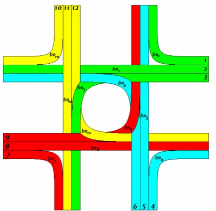
Figure 6: Schematic view of a junction
In Figure 6 all turns of a junction are depicted. Every turn has some kind of bottleneck which has a given length and returns the capacity of that turn and the maximum speed for the turn depending on the intensities of the conflicting flows and the specifics of the junction. The schematic view is always the same, whether the junction has traffic lights, is an all stop junction, roundabout or anything else. The only difference is the formula for the
i
,
i bn
.
i bn
7.1.4 Remarks
When the delay of junctions in a macro-dynamic propagation model is done in this way, it is of vital importance that the speed on the junction-segment is the correct maximum speed of a bottleneck, which depends on the delay received on that turn. Also important is that the propagation model can model the acceleration and deceleration correctly.
Acceleration and deceleration
Page 35
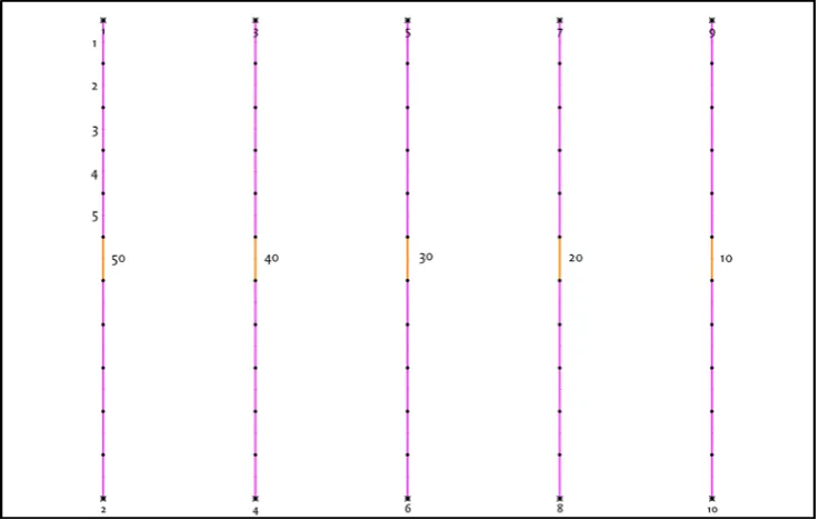
Figure 7: Testing network for acceleration and deceleration
The testing network exists of five roads all of equal length. The first five segments (from dot to dot) of each road have a length of 300 metres, the middle (orange) segment has a length of 20 metres and the last five segments are again 300 metres. The only difference between the roads is the maximum velocity on the middle segment, everything else is the same. The testing network has a maximum speed of 50 km/h on the most left road and decreases to 10 km/h on the most right. To examine the rapidity of acceleration and deceleration of MaDAM, traffic will run from the upper to the lower centroids.
Page 36
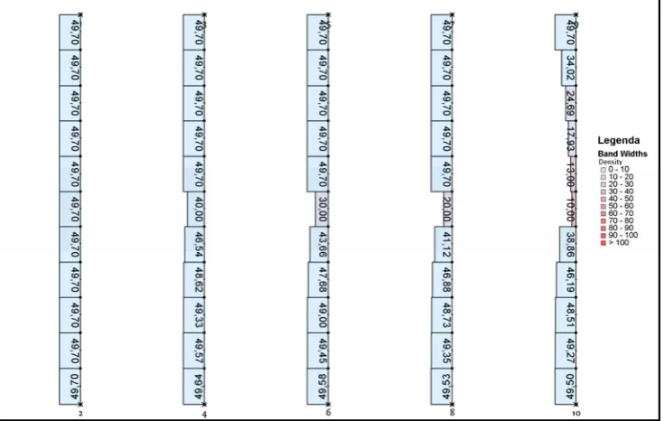
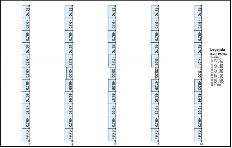
Figure 8 depicts the average speed on the segments when a total flow of 600 vehicles per hour is put on the different roads. When the flow has to slow down to a speed of 10 km/h it starts to decelerate more than 1.5 kilometres before it gets to the point where the speed limit is set. To slow down to a speed of 30 km/h, depicted in the middle road, the flow starts decelerating at approximately 1.5 kilometres before the given segment. To nullify this unrealistic braking behaviour, a smart anticipation term was implemented in MaDAM. The smart anticipation term first checks the density in the next segment and only when this is larger than half the critical density and when the anticipation term is non-negative, the anticipation term is used, otherwise the anticipation term has a value of zero. So when the density is less than half the critical density, the velocity will not drop. This can be seen in Figure 9, the velocity stays at 49.70 km/h on the first four roads. Only the last road where the density is becoming larger (a more purple colour) also has a drop in speed, though being a less drastic than the normal anticipation term.
Figure 9: Acceleration and deceleration with smart anticipation
The problem with the smart anticipation term occurs when the density on a road is approximately half the critical density. At this point the speed becomes very instable, because sometimes the density is a little lower and the anticipation term is not used, while at other times the density is a little higher than the critical density and the anticipation term is used. Also the length of deceleration is rather drastic, from no deceleration whatsoever to a deceleration for about 1 kilometre.
Page 37
Figure 10: Acceleration and deceleration with smart anticipation and junction assumptions
Figure 10 shows the average speed on links with both smart anticipation and junction-assumptions. On the first four roads, the speed-drop to allow for the extra delay is not continuous, but drops to the desired speed at the point of transition from normal road to the speed restricted road. On the last road the speed-drop is more continuous, but starts a kilometre before the road-segment with speed restriction.
Instead of the anticipation term explained in the section on Messmer & Papageorgiou, a new anticipation term can be constructed. This new anticipation term is based on the anticipation term of Payne. The section on Paynein paragraph 2.4.3, explains both this term, as well as an option of estimating the derivative of the fundamental diagram speed by means of a forward difference formula.
(
)
(
( )
)
( )
Because the anticipation term in dynamic equation (5.1.1) doesn’t give the correct result yet, an extra throughput factor is introduced:
Page 38
density on segment at time-step jam density
parameter
n
The anticipation term has to be multiplied by this throughput factor. Equation (5.1.2) has the density of the current segment as the numerator and the space still available on the next segment as denominator. Now four situations can arise:
. Both the density on this segment and on the next segment are low. When this happens, the throughput factor is small, resulting in small effect on the whole dynamic equation. In this case the difference Ve
( ) (
knj+1 −Ve knj)
is restrained, because drivers do not anticipate when there is nothing to anticipate for.. The density on this segment is low but on the next segment it is high. When this happens, the throughput factor is average, resulting in normal effect on the whole dynamic equation. In this case the difference Ve
( ) ( )
knj+1 −Ve knj is neither restrained nor magnified.. The density on this segment is high, but on the next segment it is low. When this happens, the throughput factor is average, resulting in normal effect on the whole dynamic equation. In this case the difference Ve
( ) ( )
knj+1 −Ve knj is neither restrained nor magnified.. Both the density on this segment and on the next segment are high. When this happens, the throughput factor is large, resulting in a lot effect on the whole dynamic equation. In this case the difference Ve
( ) (
knj+1 −Ve knj)
is magnified, because drivers have to anticipate when there is a lot of traffic.The constant ζis only used to calibrate the throughput factor. The anticipation term becomes:
Resulting in the complete dynamic equation:
Page 39
Figure 11: Acceleration and deceleration with Payne anticipation
The propagation model with this new anticipation term gives the results depicted in Figure 11. When a constant deceleration is assumed the flow starts braking about 50 metres before the segment with maximum speed of 10 km/h. With this assumption it takes little more than 6 seconds to decelerate from 50 km/h to 10 km/h. The acceleration takes even less time: about 4 seconds. This means that after a little less than 30 metres the speed is approximately the desired velocity again.
As mentioned in the section on Messmer & Papageorgiou, the dynamic equation used in MaDAM has some default values:
35 13 20 T
ν κ
= = =
(5.1.6)
In the new dynamic equation (5.1.5) both νand κare absent, instead a new constant is used: ζ.For the output depicted in Figure 11 the following values of the constants are used:
max 180 10 2 k
T
ζ
= = =
(5.1.7)
Page 40
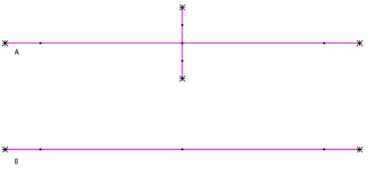
Speed on junctions
In Figure 12 two situations are shown. Situation A depicts a road from the left to the right with a junction in the middle. Situation B depicts the same road without the crossing.
Figure 12: Situations with and without crossing
The difference in travel time for the road from the left to the right, in situations A and B is the extra delay experienced on the junction in situation A. To simulate this correctly, the speed on the junction has to be adjusted in such a way that together with the loss of time for deceleration and acceleration it returns exactly the extra delay. Because a macro-dynamic propagation model adjusts the speed of the flow near bottlenecks itself, the adjusted speed on the junction only needs to take into account the loss of time for crossing the junction, it doesn’t need to consider the loss of time for the acceleration and deceleration.
To get to know the correct loss time on junctions, it is important to know how the loss time is composed. In the static Junction Modelling the loss time for a lane is computed by the following formula:
average delay on lane uniform delay on lane incremental delay on lane geometric delay on lane maximal delay on lane
When junctions are split into two classes; signalised and unsignalised, the different have the same calculations for different junction types in the same class. The difference between the classes, in a delay point of view, is the uniform delay. The incremental delay and geometric delay are the same for both classes. In the signalised class, the uniform delay depends on both the capacity of a turn and the amount of green time a turn gets.
Page 41
In the unsignalised class, the uniform delay only depends on the capacity of a turn. For the exact calculations see The explanation of Junction Modelling, which is part of Junction Modelling [Sch07].
Each of the separate delays has a different origin. The uniform delay in the signalised class is an estimate of delay, assuming uniform arrivals, stable flow and no initial queue. In the unsignalised class, the name uniform delay is badly chosen because it has nothing to do with a uniform arrival, but with the capacity of the approach lane as it is the inverse of the capacity per second. The incremental delay is an extra delay due to nonuniform arrivals, random delay and delay caused by sustained periods of over saturation. The geometric delay is the extra time needed for deceleration and acceleration, [HCM00].
This paragraph only treats a priority junction to verify whether, with the correct delay, the speed on a junction segment can be chosen in such a way that the complete travel time from one centroid to another in a dynamic model is approximately the same as in a static model.
Two different functions for the calculation of the delay are used. Both only use the incremental part of the average delay. The uniform delay part is not used because in a macroscopic dynamic traffic assignment model the speed already drops near a bottleneck. The geometric delay part is not used because the acceleration and deceleration is done in a more realistic way by the MDTA model. The first function is from the Highway Capacity Model [HCM00], the second delay function comes from the code of Junction Modelling [Sch07].
flow on the junction segment capacity of the junction segment jun
q cap
= =
The capacity of the junction segment is calculated by Junction Modelling. In this research it is assumed that the capacity given by Junction Modelling is correct.
Page 42
Figure 13: Network with priority junction
To show that the travel time in a dynamic model, with junction delay taken into account as explained, can be compared to the travel time in a static model, two times three consecutive runs are done in a static model, on a network depicted by Figure 13. The first time, a flow of 200 is set for streams from centroid 1 to 2 and flows of respectively 0, 250 and 500 are set for streams from centroid 3 to 4 and centroid 4 to 3. The second time, a flow of 600 is set for streams from centroid 1 to 2 and again flows of respectively 0, 250 and 500 for streams from centroid 3 to 4 and centroid 4 to 3. The travel time we are concerned about is that of traffic going from centroid 1 to 2.
After these six static runs, six dynamic runs are done with delay
D
HCMand six runs with delayD
JM.
In these dynamic runs, the first hour has the specified flow, the second hourPage 43
215 216 217 218 219 220 221
1 5 9 13 17 21 25 29 33 37 41 45 49 53 57 61 65 69 73 77 81 85 89 93 97 101 105 109 113 117
Time of departure
T
ravel
t
ime
Static Dynamic HCM Dynamic JM
Figure 14: Travel time; own flow 200, opposing flow two times 0
214 215 216 217 218 219 220 221 222
1 5 9 13 17 21 25 29 33 37 41 45 49 53 57 61 65 69 73 77 81 85 89 93 97 101 105 109 113 117
Time of departure
T
ravel
t
ime
Static Dynamic HCM Dynamic JM
Page 44
212 214 216 218 220 222 224 226 228
1 5 9 13 17 21 25 29 33 37 41 45 49 53 57 61 65 69 73 77 81 85 89 93 97 101 105 109 113 117
Time of departure
T
ravel
t
ime
Static Dynamic HCM Dynamic JM
Figure 16: Travel time; own flow 200, opposing flow two times 500
212 214 216 218 220 222 224 226 228
1 5 9 13 17 21 25 29 33 37 41 45 49 53 57 61 65 69 73 77 81 85 89 93 97 101 105 109 113 117
Time of departure
T
ravel
t
ime
Static Dynamic HCM Dynamic JM
Page 45
210 215 220 225 230 235 240
1 5 9 13 17 21 25 29 33 37 41 45 49 53 57 61 65 69 73 77 81 85 89 93 97 101 105 109 113 117
Time of departure
T
ravel
t
ime
Static Dynamic HCM Dynamic JM
Figure 18: Travel time; own flow 600 opposing flow two times 250
0 200 400 600 800 1000 1200 1400 1600
1 5 9 13 17 21 25 29 33 37 41 45 49 53 57 61 65 69 73 77 81 85 89 93 97 101 105 109 113 117
Time of departure
T
ravel
t
ime
Static Dynamic HCM Dynamic JM
Figure 19: Travel time; own flow 600, opposing flow two times 500
Page 46
The reason that the yellow line is not a nice parabola lies in the fact that the propagation model of Payne is a bit unstable when the speed is very low.
The delay of the Highway Capacity Model is always a bit more pessimistic. Especially in the runs where the flow from centroid 1 to 2 was 200. Here the function for the delay of Junction Modelling returned a delay of zero, resulting in a constant delay and thus a constant travel time for the first three runs.
It seems that the delay of the Highway Capacity Model is a good estimate of the reality and this could be used in the calculation of the delay in a macroscopic dynamic traffic assignment model.
7.2
Schematics of the algorithm
Page 47
MDTA
Junction model
Update?Done? No
No
Yes
Output
YesPreparation
Begin
Figure 20: Flow-chart of X-Stream in MaDAM
A simplified flowchart of the process of a macroscopic dynamic traffic assignment model is depicted in Figure 20. The parts which are important for X-Stream are coloured blue.
7.3
Calibration and validation
A distinction has to be made between the calibration and validation of the new anticipation term and the validation of the effects of junctions, i.e. the delay and capacity. It is recommended that the new anticipation term (5.1.5) is not only used for intersections, but for the complete urban network. This recommendation is not only made because the anticipation term should have effect before and after the intersection, but also because it seems to approach reality in a more realistic way than the old anticipation term. The new anticipation term has to be calibrated and validated for an urban network, not just for intersections. The effects of junctions are only of importance on junctions and need therefore only be validated on junctions.
7.3.1 Propagation model with new anticipation term
Page 48
Three speeds have to be measured. Firstly the average vehicle speed on a segment 200 metres before the speed bump. Secondly the speed with which the vehicle crosses the speed bump. Thirdly the average vehicle speed on a segment of 200 metre after the speed bump. When this is done for say an hour, the number of vehicles passing the speed bump has to be counted. An hourly average speed on the segments and on the speed bump can now be calculated. A network can then be made of a road say two segments long befor