Extended Analysis of Back Testing
Framework for Value at Risk
Internship Rabobank International
author:
G.J. van Roekel
study:
Industrial Engineering and Management
track Financial Engineering
department:
Finance & Accounting
supervisors:
Emad Imreizeeq MSc. (University of Twente)
dr. Berend Roorda (University of Twente)
dr. Viktor Tchistiakov (Rabobank International)
Wei Lan MSc. (Rabobank International)
MASTER THESIS EXTENDED ANALYSIS OF BACK TESTING FRAMEWORK 3
E
XECUTIVE
S
UMMARY
-at-Risk model and the back testing procedure are important parts of the banks market risk framework. The Value-at-Risk model provides a daily measure th
exceed once every 100 days.
DNB and Rabobank agreed to perform a periodic analysis of the VaR model that goes beyond the regulatory guidelines. Every quarter Rabobank International tests the accuracy of its VaR model using the regulatory back test. This back test checks the number of times the VaR was breached (called exception). Based on this number of exceptions this test judges if the VaR model is accurate or not. The regulatory back test has its limitations.
Therefore, we conducted a literature research to investigate alternative back test methods. This resulted in a framework of five back tests that together test the most important properties of a VaR model:
- exception frequency: the number of realised exceptions
- exception clustering: independency of exceptions over the tested period. - exception size: the size of the exception
We implemented the five back tests in a test framework that Rabobank International can use for the periodic back testing beyond regulation.
6 MASTER THESIS EXTENDED ANALYSIS OF BACK TESTING FRAMEWORK
8.3 Implementation ...43
8.4 Test results ...43
9Other Back Testing Methods ... 44
9.1 Test Descriptions ...44
9.2 Selection...45
10 Test Conclusions Summary ... 46
11 Alternative VaR Models... 47
12 Implications Future Research... 48
12.1 Exception clustering...48
Literature ... 49
Appendix A. Keywords Search ... 52
Appendix B. Power POF test ... 53
Appendix C. Model Overview ... 54
Appendix D. Implementation... 57
MASTER THESIS EXTENDED ANALYSIS OF BACK TESTING FRAMEWORK 7
1
I
NTRODUCTION
Rabobank International uses the Value at Risk (VaR) model to determine and control the exposure of the bank to market risk. De Nederlandsche Bank (DNB) expects Rabobank to use this model and to test its accuracy. Rabobank International agreed with DNB to perform periodical tests that move beyond strict regulatory guidelines. Next to that, the subprime crisis has led to very volatile financial markets. It is important for Rabobank International to know if their current model is good enough to represent this extraordinary market situation. During the internship I worked within Rabobank International to test the accuracy of the risk m odel.
The above description is technical and contains terms that need additional explanation. The next sections of the introduction provide an overview of the context of the project. It starts at a high level with a general description of financial risk management. Thereafter it explains market risk and the VaR framework for measuring market risk. It ends with the explanation of the tests to measure the accuracy of VaR.
1.1
Financial Risk Management
Risk plays an important role in life and especially in business activities. A general definition of risk is The next step is to narrow the scope of the definition to the risk that organisations are exposed to. This risk can be split into two types: business risks and non-business risks. Business risks are risks that an organisation is willing to take for the creation of a competitive advantage and add value for shareholders. Non-business risks are risks that are not directly related to the core business.
For a financial firm a main part of business risk is financial risk. This is the risk that relates to possible losses in financial markets. Financial markets are the places for trading diverse financial products like FX, equity and credit spreads. In order to cope with this risk, financial firms have extensive and intensive accurate risk measurement and risk management.
1.2
Market Risk
1.2.1
Definition
If we look into more detail into financial risk, we can divide it in the following risk categories:
- market risk: risk that arises from movements in the level or volatility in market prices
- credit risk: risk caused by the fact that companies may be unwilling or unable to fulfil their contractual obligations
- liquidity risk: risk that the bank cannot do a trade because the size of the trade is too large relative to the market size (asset liquidity risk) or risk that the bank has not enough cash available to fulfil payments obligations (funding liquidity risk)
The purpose of the project is to test the used model for market risk. So we look in more detail at this specific category of financial risk. Rabobank International trades lots of different financial products. The bank categorises these products in trading books.
Changes in market prices influence the value of financial products and create market risk for the holder of the products. Market prices are for example interest rates, exchange rates, equity prices and commodity prices. It is important for a bank to know to what amount of market risk it is exposed to, because it wants to control the risks
1.2.2
VaR history
8 MASTER THESIS EXTENDED ANALYSIS OF BACK TESTING FRAMEWORK
In the past, several techniques were used to measure market risk. These measurements all had clear limitations and were not capable of giving a single good indication of how big risk exposure was.
summarised the market risk of a certain portfolio in a single number. They used it several years internally before they made i
adopted by many organisations, also because the Group of Thirty recognised VaR as a best practice. The Group of Thirty represents the largest banks in the world. Initially, their main goal was to develop a framework for best practices to deal with derivatives. A rapid growth was visible in the market for derivatives. A derivative is a security whose price is dependent upon or derived from one or more underlying assets (Investopedia, 2008). Well-known types of derivatives are options, swaps, futures and forwards. These products are traded very easily and provide the opportunity to take potentially large positions in the underlying assets with an investment that is relatively small. The value of the underlying assets is affected by changes in market prices. This value change can be very high in comparison to the investment in the derivative. So, the exposure to market risk can be quite high for derivatives.
-at-Risk as the best method for measuring market risk.
Regulators of the financial industry were also investigating a uniform (market) risk management framework. They were thinking how to oblige banks and other financial institutions to carry enough capital to provide cover for incidental large losses.
A first step that has been taken by regulators, to unify rules and policy, is the development of the Basel Capital Accord (BCBS, 1988) by the Bank for International Settlements. The goal of this document was to define a standard for minimal capital requirements that banks should hold to cover their risk exposure. One of the limitations of this document was that it contained few guidelines or rules for market risk. This was solved by the Committee with a so-called Amendment to the 1988 Accord (BCBS, 1996). This document obliged the banks to either use a standard model or an internal model to determine the minimum amount of capital that has to be reserved to cover market risk. The internal model produces a VaR as measure of market risk. Because most banks adopted internal models and the regulators prescribed its use in that case, VaR has become the industry standard for measuring market risk. Rabobank International also implemented an internal VaR model.
1.2.3
Definition VaR
VaR is a value that summarizes the worst loss over a target horizon with a given level of confidence. VaR does not indicate how large the expected loss will be under the worst case scenario. Instead, it is a border value that will be crossed no more than a given number of times, depending on the confidence level.
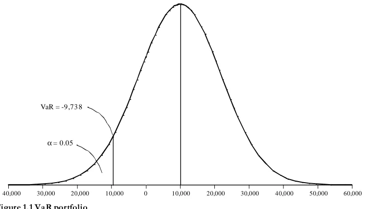
By means of an example, we will try to explain this. The daily return of this portfolio is assumed to be normally distributed with mean 10,000 and standard deviation of 12,000.
MASTER THESIS EXTENDED ANALYSIS OF BACK TESTING FRAMEWORK 9
Figure 1.1 VaR portfolio
The figure shows the probability density function of the daily return of the portfolio. The figure indicates the surface corresponding with the lower 5% of this distribution by . The VaR measure that is the border of this surface indicates that in 5% of all realised returns, the realised return will be smaller than or equal to -9,738. This value is the 95% confidence level VaR measure.
1.3
Testing VaR
We described in the introduction that DNB requires Rabobank International to test its VaR model. This section describes why DNB, in its function as a regulator, wants the banks to test the VaR model and it introduces the method that is used to perform this test.
Although many organisations and institutions accept and use VaR as a market risk measure, it does have its limitations (Jorion, 2007):
- VaR does not describe the worst loss, but represents a value that will be exceeded in a certain number of trading days over a given period (5 of 100 days in case of a 95% VaR confidence level).
- VaR does not give any information about the distribution of the losses in the lower tail. So if the VaR is exceeded only with a small amount or with a very large amount will not be shown.
Due to these limitations, DNB is very interested to see if the results of a VaR model are accurate. This has become even more important since the subprime crisis has had a large influence on the performance of banks. Several banks in the United States and Europe suffered large losses during the subprime period and it is very interesting for the central banks to see if the VaR models worked well in these circumstances.
s accuracy is back testing. We showed that a VaR model provides a loss limit that will be crossed a number of times in a certain time range. Regulators designed the back testing method to check if the number of realised exceptions (breaches of the VaR) over a given period of time is statistically not significantly different from the expected number of exceptions. For example, if the number of exceptions is too high, this can be reason for a regulator to ask a bank to provide additional insight in the model or force it to develop an improved model.
Next to this evaluation function, back testing also has implications for the capital requirement the regulator sets for the bank. The capital requirement is an amount of money a bank has to hold to cover its risk positions. The use
40,000 30,000 20,000 10,000 0 10,000 20,000 30,000 40,000 50,000 60,000
10 MASTER THESIS EXTENDED ANALYSIS OF BACK TESTING FRAMEWORK
MASTER THESIS EXTENDED ANALYSIS OF BACK TESTING FRAMEWORK 11
2
P
ROJECT
D
EFINITION
In this chapter we define exactly what the project is about and which steps will be taken to reach the goals set. The first section discusses the project objectives. Next we determine the scope. To reach the objectives, we develop a research model and research questions. The final section provides an overview of the structure of the thesis.
2.1
Project Objectives
The following statement represents the project objectives that we want to reach:
The main objectives of the research are to develop a tool for thorough back testing, to use the tool to analyse the performance of the VaR model and provide recommendations for improvements of the VaR model.
By fulfilling this objective we investigate the main problems mentioned in the introduction. First of all, the project provides Rabobank International with a tool that they can use periodically to report to DNB a thorough risk analysis and to gain additional insight in the performance of the VaR model. Next to that, the study provides an analysis of the current VaR model given the results of the back tests that we perform with the tool. We perform the back tests in such a way that we can analyse the influence of the subprime crisis. Finally, we make an initial investigation of alternative VaR models.
2.2
Scope
We perform the back tests on a number of trading books. Experts of Rabobank International make this selection such that it is a good representation of all major risk categories. The results of the back test provide insight in the performance of the current VaR model. Based on this, we investigate improvements for the VaR model and perform initial research into VaR model alternatives. A complete redesign of the VaR model is not within the scope of this project.
2.3
Project Structure
12 MASTER THESIS EXTENDED ANALYSIS OF BACK TESTING FRAMEWORK
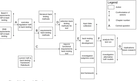
Figure 2.1 Research Flowchart
We specify this research flowchart by developing seven central research questions. Each specific research question connects to the corresponding letter in the research flowchart. The numbers above the action blocks give the chapter in which this issue is discussed.
A. What are the regulatory requirements for back testing and VaR? (Ch. 3 & 4) B. What are the requirements for suitable back testing methods? (Ch. 5)
C. What are the input and functional requirement for the new back testing tool? (Ch. 5)
D. Which back testing methods are suitable for implementation in the new tool? (Ch. 6, 7, 8 & 9) E. How can we develop the new tool? (Ch. 5)
F. What conclusions can we draw from the initial test run? (Ch. 10)
G. What implications for future research can we make up based on the initial investigation into alternative VaR models? (Ch. 12)
2.4
Thesis Structure
We derive the structure of the thesis in a straightforward manner. First of all, we provide a detailed description of the regulation for VaR and how it is implemented at Rabobank International in Chapter 3. Chapter 4 discusses the regulation for back testing VaR and its implementation. Chapter 5 gives an overview of the back testing 6 discusses the exception frequency back tests. We describe the second category of back testing methods, exception clustering, in Chapter 7. Chapter 8 discusses the exceptions size back tests. We describe methods that do not fall in one of the previous categories in Chapter 9. Chapter 10 contains a summary of the conclusions we obtain from the first test run. Chapter 11 provides an overview of the alternative VaR models we investigated. Chapter 12 contains the implications for future research.
MASTER THESIS EXTENDED ANALYSIS OF BACK TESTING FRAMEWORK 13
3
V
ALUE AT
R
ISK
In this section we first give an overview of the regulation that relates to VaR. Next we describe the most used methods for determining the VaR.
3.1
Regulation
In the Basel Committee on Banking Supervision different institutions from the international banking world work together to overcome regulatory issues. The cooperation between banks is meant to upgrade the quality of worldwide regulation. This section provides an overview of the regulation, relating to VaR, that the Committee has developed in their most recent regulation document (BCBS, 2006). The numbers between brackets indicate the section number of the document. The document allows banks to use two methodologies to measure their market risk. The first is the implementation of a standard model that the document prescribes. The second choice is to use an internal model. Most banks prefer to use this internal model, since it is a better reflection of diversification that (Hull, 2007). In order to use the internal model the bank has to fulfil a set of demands (701(ii)). Among these demands is the requirement to compute the VaR on a daily basis. The levels of VaR that the bank has to measure are the 10-day period 99% percentile and the 1-day period 99% percentile. The bank can use these VaR levels to respectively determine the capital requirement for market risk and obtain the multiplier for this capital requirement.
3.2
VaR methods
The regulator does not prescribe the method to compute the VaR. A bank is free to choose its own method. Many methods exist, but we can disseminate three main types of methods. We describe these in the next subsections.
3.2.1
Variance / Covariance method
J.P. Morgan adopted this method in
a lot of different financial products. Market factors like interest rates, stock prices and currency rates influence the value of each of these financial products. The variance / covariance method uses estimates for the volatilities of the market factors and the correlations between market factors to obtain an
overall portfolio. The RiskMetrics method uses approximations to determine the volatility for more complicated financial products. The method assumes the overall portfolio has a normal distribution with mean zero and the estimated volatility. Finally, one estimates the VaR for the overall portfolio by taking the 99% percentile of this distribution.
3.2.2
Historical Simulation
Historical Simulation uses a set of data from the past to give a prediction of what will happen in the future. To be more specific, in this method we use a history of e.g. 250 hypothetical market factor shocks to determine what the portfolio VaR for tomorrow is. We compute the VaR by taking the 99% percentile of the hypothetical market shocks.
3.2.3
Monte Carlo Simulation
14 MASTER THESIS EXTENDED ANALYSIS OF BACK TESTING FRAMEWORK
3.3
VaR at Rabobank
MASTER THESIS EXTENDED ANALYSIS OF BACK TESTING FRAMEWORK 15
4
B
ACK TESTING
V
A
R
Regulation prescribes that all banks, that use an internal model for the measurement of their market risk exposure, should verify the quality of this model using the so-called back testing procedure. This chapter gives an overview of the precise demands of the regulation of Basel II and DNB in the first and second section. The third section describes how the back testing procedure is applied at Rabobank.
4.1
Basel II Regulation
The first subsection summarises why back testing is necessary. Subsection two contains a description of the back testing framework prescribed by the Committee. Finally, the third subsection describes how banks should interpret the results of the back tests. The numbers between brackets refer to the paragraph numbers of the Basel II regulation document (BCBS, 2006).
4.1.1
Need for Back Testing
If a bank chooses to develop an internal model for market risk, one of the requirements of the Basel II Accord is that they have to implement a back testing procedure (718(LXXIV)(b)). Through this method, the regulators can gain insight in and judge the performance of the internal models used at the banks.
Many methods exist for back testing; no uniform method gives the best results. This is something the Committee has taken into account while developing the regulation. The goal of the back testing procedure is to find a balance between its performance in measuring power and its imperfections (Annex 10a.6).
Back testing is especially important since it is the most important factor in determining the capital requirement that banks have to hold to cover market risk of their trading portfolio. The size of the capital requirement is equal to the higher value of the VaR of the day before and the average of the VaR values of the previous sixty days multiplied by a factor (718(LXXVI)(i)). The multiplication factor has a minimum value of 3 and can be as high as 4, depending on how good or bad the results of the back tests for the actual P&L are (718(LXXVI)(j)). The amount of regulatory capital for market risk can be calculated with the following formula:
(4.1)
The VaR measure used here is the 10-day 99% confidence level VaR.
The Basel II document also prescribes additional tests that banks have to perform next to the standard back test (718(XCix)). Firstly, they must demonstrate that all assumptions in the model are appropriate. Examples of assumptions are the use of a normal distribution and the use of the square root of time rule for scaling from a one-day to a ten-one-day holding period of the VaR. Tests for model validation should go beyond the standard Basel II back test. Specific examples that the regulation gives are:
- Perform back tests with hypothetical changes in portfolio value. - Perform back tests over a longer look back period.
- Use other confidence intervals than the 99% interval required. - Test portfolios below the bank level.
16 MASTER THESIS EXTENDED ANALYSIS OF BACK TESTING FRAMEWORK
4.1.2
Basel II Back Testing Framework
The Basel Committee developed a standard minimum test that banks should perform in measuring their market
Basically, back testing is simply about a periodic comparison of the banks daily VaR measures and the actual trading outcome for that day (Annex 10a.8). The framework requires banks to compute VaR at a confidence level of 99% (Annex 10a.10). Given this confidence level we expect that once every 100 days the actual trading loss is larger than the VaR. We call this breach of the VaR an exception. By simply comparing the realised number of exceptions with the expected number we can draw conclusions upon the performance of the VaR model.
An important limitation of the described back testing method is the fact that it uses the actual trading result of a day in the comparison with the VaR estimate. This assumes that the only changes that take place during the day are due to price and rate movements. This does not happen, since portfolios change during the day. So the actual trading results include fee income and trading gains and losses. These values contaminate the back test results (Annex 10a.12). Because of this reason the framework uses VaR with a one-day holding period. A ten-day holding period would include even more trading events and portfolio changes.
The framework suggests some solutions that might (partially) solve the contamination problem. The first one is eliminating the contamination by carefully identifying the contaminating values and leaving them out of the back test. The second solution consists of using hypothetical instead of actual trading results. The bank computes hypothetical results under the assumption that during a trading day the positions in the portfolio do not change. By using this method, all changes in portfolio value happen due to changes in market factors like interest rates.
Regulation requires banks to perform the back test quarterly using at least a year of trading data (Annex 10a.22). A limitation of the back tests formulated by the Committee is that they cannot distinguish accurate and inaccurate models extremely well (Annex 10a.26). On the other hand it is very easy to implement and perform.
4.1.3
Interpretation Results
Now that the back testing method is clear, we address how the results should be interpreted according to the Basel II Accord (Annex 10a.27-59).
Since the back test does have its limitations, one cannot implement very strict rules for judging the model. Otherwise the probability of a type 1 error (rejecting an accurate model) or a type 2 error (accepting an erroneous model) would become too large. Instead, regulation prescribes three result zones: green, yellow and red. The green zone indicates that the number of exceptions generated by the model is acceptable and suggests the model is accurate. The yellow zone will start a discussion of the results. Exceptions might be attributed to multiple causes (Annex 10a.48):
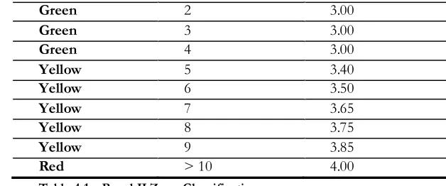
In case of the yellow zone, the bank will get a chance to prove that the high number of exceptions has another cause than an inaccurate model, before the regulator raises the multiplication factor. Finally, the red zone involves such a high number of exceptions that the probability of an accurate model is very low. In that case, the regulator penalises the bank with an increase of the multiplication factor to 4 and the requirement to develop an improved model. Table 4.1 contains an overview of the zones, number of exceptions and the size of the multiplication factor.
Zone # Exceptions Multiplication factor
Green 0 3.00
MASTER THESIS EXTENDED ANALYSIS OF BACK TESTING FRAMEWORK 17
Table 4.1 Basel II Zone Classification
4.2
European and DNB Regulation
The European Union implemented much of the Basel II requirements in law in the Capital Requirements Directive (CRD). This again is transferred in Dutch Law into the Financial Supervision Act (FSA). Finally, DNB transferred the annexes of the CRD into regulation. Of special interest to this paper is regulation that is prescribed by DNB (DNB, 2006).
4.2.1
Regular Validation
DNB wants the banks to validate its internal model both periodically and in special cases. The periodical requirement states that the banks should validate its model at least once a year or in special cases. Special cases involve significant changes to the model or market events that are likely to have a large influence on the model and maybe even make the model inaccurate.
To validate the internal model, banks should use other techniques besides back testing. The DNB requirements oblige the bank to perform at least:
- tests to demonstrate that any assumptions made within the internal model are appropriate and do not
under- or overestimate the risk;
-- the usage of hypothetical portfolios to ensure that the internal model is able to account for particular
structural features that may arise.
DNB also recognises the contamination problem which we mentioned in subsection 4.1.2, because they require the banks to include both actual and hypothetical profits and losses in the back testing procedure.
The last part of the regulation that is important for back testing has to do with the results of the back test. DNB also allows banks to ask for dispensation from capital requirement increases. But regulation states very clearly that this can happen only under exceptional circumstances. Next to that, if a bank experiences inaccuracies in the VaR model through back testing, DNB should be notified in five days.
4.3
Back Testing at Rabobank International
18 MASTER THESIS EXTENDED ANALYSIS OF BACK TESTING FRAMEWORK
5
B
ACK
T
ESTING
F
RAMEWORK
R
EQUIREMENTS
This chapter gives an overview of the back testing framework that we develop in the project. We divide the methodology part of the project in three major fractions, which are described in the three sections of this chapter. The first part is the back test method research, in which we investigate which back testing methods are most suitable for implementation. The second part is the tool development for which we set up a list of requirements. Finally, the third part is the test framework which describes how we design the first test run.
5.1
Back Test Method Research
To obtain the most suitable back testing methods for the new back testing framework, we perform a literature study. The first two subsections describe how we perform the research and what scope we use. We set up a number of requirements for the back testing methods that we discuss in the third section. Finally, the fourth section describes how we make the selection.
5.1.1
Research Method
In order to provide a decent overview of suitable methods, we use a structured approach. The starting point is the detailed overview of VaR by Jorion (Jorion, 2001). This book dedicates a chapter to back testing. This provides us insight in the more basic tests and types of methods. Next to that it gives references to basic articles on back testing (Kupiec, 1995), (Christoffersen, 1998), (Crnkovic and Drachman, 1997) (Lopez, 1999). The next step we perform is searching the articles citing these authors. We find existing literature reviews on back testing methods (Campbell, 2005), (Haas, 2001), (Blanco and Oks, 2004). Also, we discover an extensive list of articles describing one or more back testing methods. To provide a thorough literature research, we also use two major search engines (Scopus, 2008) (ISI, 2008) with a list of keywords (found in 0). Together, these search engines cover almost 25.000 journals (Scopus, 2008) (ISI, 2008). Finally, we use the web site of GloriaMundi, containing a list of 57 articles on back testing VaR (GloriaMundi, 2008). Our analysis consists of scanning, selecting and summarising back testing methods from this extensive collection of articles. This results in a division of the back testing methods into three different types: exception frequency, exception clustering and exception size. Each type tests a different property of the VaR model. In the Chapters 6, 7 and 8 we discuss each of these types. Finally, Chapter 9 contains methods that do not fall under one of the other three types.
5.1.2
Scope
A distribution back test that compares the realised and hypothetical distribution has more power in detecting an inaccurate model than the methods that only address a quantile of the distribution (Campbell, 2005). But the increased power comes at a cost. Campbell states that a VaR model can excel in describing extreme losses but be less accurate on moderate profits and losses. In that case, we could judge the model as inaccurate, while the model is accurate from a risk management perspective. For this purpose, we are first of all interested in the properties of
MASTER THESIS EXTENDED ANALYSIS OF BACK TESTING FRAMEWORK 19
5.1.3
Requirements
An ideal back testing method does not exist. In order to make a good selection of back testing methods we set up a number of requirements. We investigate for each back testing methods how it performs for each of the requirements.
The requirements we use are goals, power, size and feasibility. The following subsections provide an explanation of each of these four.
Goals
For each method we define what the goal of the test is. The requirement this goal.
Power
Statistical tests always are a trade off between the two types of errors that can arise. A good statistical test has both a low type 1 and type 2 error. A type 1 error occurs if the null hypothesis is true, but rejected by the test. The type 2 error occurs if the null hypothesis is false, but accepted by the test.
In case of most back tests the errors are rejecting an accurate model (type 1) and accepting an inaccurate model
(type 2 how good the
back test is in separating inaccurate and accurate models.
Size
The sample size is the look back period, measured in trading days that we use as input for the back tests. Some of the back tests require large sizes in order to make sure the results of the test are reliable in separating inaccurate and accurate models. This is not very convenient, since we would like to see reliable test results also for short look back periods.
If a test needs a large sample size for accuracy, we give a low score for the size criterion. If it needs only a small sample size, we give it a high score.
Feasibility
The feasibility criterion covers some topics that we cannot measure easily:
- If the added value of the test is large enough to overcome the implementation effort.
- If the back testing method tests a property of the VaR model that is not or partially covered by other
methods.
5.1.4
Selection Procedure
20 MASTER THESIS EXTENDED ANALYSIS OF BACK TESTING FRAMEWORK
This section describes the requirements that we set up for the back testing tool. The first subsection contains the domain analysis which describes the environment in where expert will use the tool. In the next subsection we determine the input requirements for the tool. In the section after that we discuss the functional requirements, which describe the user settings that have to be available in the tool. Finally, we give an overview of the output the tool has to generate.
5.2.1
Domain analysis
Experts within Rabobank will use the tool for two main purposes. The first one is the reporting Rabobank International has to fulfil to De Nederlandsche Bank (DNB). This has to show how well the VaR model for market risk within Rabobank International performs. The current procedure measures this model performance by back testing. Every quarter DNB requires Rabobank International to deliver a report containing a description of the results of the Basel II back test for individual trading books within Rabobank International and at an overall group level. Besides this quarterly report, Rabobank International promised DNB to provide regular additional insight in the
. Experts can use the tool that we develop in this project to provide this additional insight.
Secondly, experts can use the information that the back testing tool provides to judge the performance of the VaR model and the individual trading books.
5.2.2
Input Requirements
We have to make decisions on what data we will use as input for the tool. In this section we give an overview of the data that we will use in the first test run. We create this overview with a description of the requirements concerning the selection of the trading books and the input data structure.
1. The input data for the first test run must contain a representative selection of Rabobank
International
We perform the initial test run over a number of trading books that is representative for the group level portfolio. In section 1.2 we mentioned four categories of market prices: equity, interest rate, commodity and FX. Rabobank International has also divided its trading books in these four categories. We do not select the trading books ourselves, but a representative selection of the categories has been made by experts of Global Market Risk. The books that they selected have the highest contribution to the group level VaR.
2. The tool must be able to handle different trading books.
We want to use the first selection of the trading books to investigate how well the VaR model performs for trading portfolios from different risk categories, especially during the subprime crisis. But Rabobank International should be able to use the tool after the project. So the tool must be able to cope with other trading books as well.
MASTER THESIS EXTENDED ANALYSIS OF BACK TESTING FRAMEWORK 21 We include this requirement because of regulation. Basel II requires a bank to use both hypothetical and actual profits and losses in their back testing procedure.
4. Four types of VaR coverage have to be tested (1-day 95%, 97.5% and 99% & 10-day 99% coverage)
The data that we need for the tool is extracted from a VaR database, risk engines and a control database within Rabobank for each trading book. The VaR coverage levels that we use are the estimated 1-day VaR values at 95%, 97.5% and 99% coverage and the 10-day VaR at 99% coverage.
We need to include the 1-day VaR at 99%, since this is the level that banks have to use for back testing due to regulation.
We include the 97.5% because Rabobank International incorporated this measure. The back testing might be used for internal model control, so inclusion of this measure is appropriate.
We include the 95% because we decided to leave out back testing methods that use distribution forecasts. One argument for this decision was that we would include multiple VaR levels in the tool.
We include the 10-day 99% VaR measure since the bank uses this value for determining the Basel II capital requirement as mentioned in section 4.1.1.
5. The look back period taken into account in the back tests should range from 250-1250 days.
The look back period is the number of days we take into account in the back testing procedure (sample size). We want to test for different periods to see if the length of the period influences the test results.
To determine the input data requirements we need to set an upper limit to the number of days that can be judged by the back testing tool. This limit is set to 1250 trading days, equivalent to 5 years. Since both short and long look back periods have drawbacks, testing scenarios have to include periods ranging from 250 to 1250 days.
6. The initial test data set will include records until April 1st 2008.
By using this end date, we make sure that recent data is tested. The subprime crisis started around August 2007. Using the 1st of April 2008 as end date, the amount of data representing the sub-prime crisis is large enough to test
model accuracy during that period.
5.2.3
Functional Requirements
The tests that we will
the possibility to set the values of several of these parameters. This makes the tool very flexible and allows for extensive scenario testing. This section describes the options that the end user has in selecting the test parameters.
7. The user should be able to select back tests to be performed individually (optional)
All of the tests we will select are separately selectable. It is not necessary to include all back tests in each test run.
8. The user can select the size of the look back period in the range of 250-1250 days. (optional)
For each test run the user selects a single amount of days. This means that if a user wants to test multiple look back periods of different length, it will be necessary that he performs multiple test runs. This reduces flexibility, but it also makes the implementation simpler. This requirement is optional, since the user can also influence the size of the look back period using the input data.
9. The user can select an end date for the look back period. (optional)
We include this option so that the user is able to select look back periods that end before April 1st. This is
especially useful to test different scenarios in- and excluding the sub-prime crisis. This requirement is optional, since the user can change the end date by altering the input data.
10. The user has the option to exclude actual or hypothetical profits and losses. (optional)
22 MASTER THESIS EXTENDED ANALYSIS OF BACK TESTING FRAMEWORK
5.2.4
Output Requirements
The tool will provide an overview of the results. The following requirements indicate what outputs the tool should provide and why.
11. The outputs should contain summary statistics of the selected P&L types and VaR coverage
levels.
The statistics can provide quick insight into the size, volatility and distribution of the P&Ls and VaR levels.
12. The selected P&L types and VaR coverage levels have to be represented in graphs.
A graph in which the profits and losses and VaR are set out over the look back period can provide quick insight into the development of these values over time.
13. The output overview should provide the number of exceptions.
The back testing tool is all about the exceptions, so the number of exceptions that occurred should be part of the output. We make a distinction between ex Rabobank International also uses this limit in the current back testing tool. The tool uses all exceptions to measure the accuracy of the VaR model, 50,000 more thoroughly and they provide argumentation to explain why it occurred.
14. The tool should present the results of all tests using a zone classification.
No matter what tests we select, the tool should present the test results in such a way that the user can see immediately how the test classified
red zone is very convenient for this. If applicable, we will use the same kind of zone classification for the tests that we select for implementation.
5.3
Test Framework
The research objective states that the tool developed should be
ction describes the test procedure that we followed. The second section describes how we interpret the results of tests.
5.3.1
Test procedure
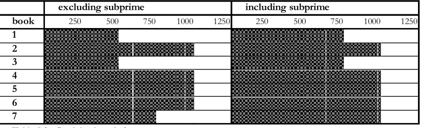
The input data set for the first test run contains the P&L and VaR vectors for seven trading books. There is not enough trading book data available to test all look back periods ranging from 250 to 1250 data points. Table 5.2 gives an overview which look back periods we test for the books.
MASTER THESIS EXTENDED ANALYSIS OF BACK TESTING FRAMEWORK 23 Next to the different look back period lengths, we make a distinction between periods including and excluding
st st April, 2008.
We test the trading books for four VaR levels (99% 1-day, 97.5% 1-day, 95% 1-day and 99% 10-day). We test the trading books for the actual and hypothetical P&L.
5.3.2
Results analysis
In order to test more specifically how the VaR model performs, we set up several detailed analyses. Although the individual book results will be available from the output of the tool, we do not discuss the performance of the individual books.
results are out of the scope. Nevertheless, these results can be important for internal purposes within Rabobank
International .
The first analysis that we conduct for each implemented back test simply creates an overview of all observations. As tests are run on a wide variety of portfolios and VaR percentiles, the graphs in which we present the results do not show individual outcomes. Instead, they present the percentages of the observations that fall in a particular zone.
The number of observations that we present in the results depends on the number of parameters that is taken into account. We provide the number of observations for each test in the graph, since the number of observations is not equal for all tests. For example, each book has a different maximum look back period (see Table 5.2), so the comparison amongst look back periods will show a different number of observations for each look back period.
We assume that Rabobank International odel is correct, so we can compare the percentage of realised results in the different zones with the expected percentage. For each back test we add a table that describes the zone classification in the section that gives the results overview.
We perform additional analyses to test more detailed factors that can influence the performance of the VaR model. The next sections describe these additional analyses.
5.3.3
Difference between actual and hypothetical P&L
P&L types have a very different interpretation. Hypothetical P&L is based on the same market data, position data and pricing models as the VaR computations. So the back testing results of the hypothetical P&L explicitly show how good the model used for VaR calculation is.
The actual P&L is influenced by portfolio changes during a trading day. Back testing provides insight in the accuracy of position data, market data and pricing models combined.
Due to the large differences in interpretation, each of the additional analyses is split into actual and hypothetical P&L results.
5.3.4
Influence of the subprime period
We make a comparison between the test results for the period preceding July 2007 (excluding the subprime crisis) and the period preceding April 2008 (including the subprime crisis).
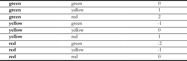
In the tool requirements we mentioned that we include a zone classification for all tests we select. We compare results from both periods with the same parameters (look back period and VaR level). We do this by checking the zone in which the results fall and scoring the difference in zones. For example, if the result excluding subprime falls into the green zone and the result including subprime is in the red zone the comparison score is 2. Table 5.3 represents the scores that we attached to each difference in zone classifications.
zone classification (excl. subprime)
zone classification (incl. subprime)
24 MASTER THESIS EXTENDED ANALYSIS OF BACK TESTING FRAMEWORK
green green 0
green yellow 1
green red 2
yellow green -1
yellow yellow 0
yellow red 1
red green -2
red yellow -1
red red 0
Table 5.3 Scoring procedure subprime comparison
5.3.5
VaR percentage level influence on results
We made the decision to exclude back tests that test the distribution of the underlying P&L distribution. To compensate for this exclusion, we include different VaR levels in the back testing tool. By including 99%, 97.5% and 95% VaR levels, we can test a larger part of the tail of the VaR model. If the results are very different for each VaR level, this might indicate a weak VaR model.
We take all the model results of the individual trading books together and then split according to the four VaR levels. Recall that we will give the number of observations for each VaR level in the result charts. Since every VaR level has an equal number of model results, we graph the test results in a stack diagram summing to a total of 100%.
5.3.6
Look back length influence on results
High confidence level VaR models like the 99% model generate only few exceptions. We expect that a larger look back period will generate more reliable test results. So, we are interested to see if the length of the look back periods influences the test results. That is why we compare several look back period lengths.
MASTER THESIS EXTENDED ANALYSIS OF BACK TESTING FRAMEWORK 25
6
E
XCEPTION
F
REQUENCY
T
ESTS
The most basic type of back testing checks the unconditional coverage or frequency p roperty of the VaR models (Campbell, 2005). This type of test considers the frequency of exceptions that was realised during a period and compares this with the number of exceptions that one would expect given the confidence level of the VaR model. This type of test only considers the number of exceptions. It does not make a difference how the exceptions are divided over time or how large the exceptions are.
For example, if a VaR model has a confidence level of 99% and we consider a period of 250 days, one would expect that during this period, in 2.5 days the model would realise a loss that is larger than the VaR. If the realised frequency of exceptions is six, exception frequency tests will analyse if an inaccurate VaR model caused that number.
This chapter gives an overview of the exception frequency tests that we discuss in this project. The first section describes the details about the methods we encountered during the literature research. The second section contains the selection of the methods that we implement in the tool. The third section describes what choices we made in the implementation of the tests. Finally, the fourth section gives an overview of the results of the initial test run.
6.1
Test Descriptions
In this section we describe the exception frequency tests we investigated in the literature research. For each back test we first give a general description of the test. The goal is one of the requirements that we use in the test selection. Next, we indicate what the underlying distribution of the exceptions is. After that we indicate what the test measur
errors are. Large errors mean low power of the test. Finally, we describe what the influence of the length of the look back period on the test results is.
6.1.1
Basel II Back Test
Description
The Basel II back test is the most commonly used back test. The regulator requires banks to use this method with a look back period of 250 days. For each of these days the bank has calculated a VaR and P&L. With the 99% confidence interval level that this test uses, the expected number of exceptions is 2.5 during the look back period of 250 days.
Goal
goal is to find out if the VaR model is accurate by testing the number of exceptions that is generated. It regards a model as accurate if the realised number of exceptions is not significantly larger than the expected number of exceptions.
Exception Distribution
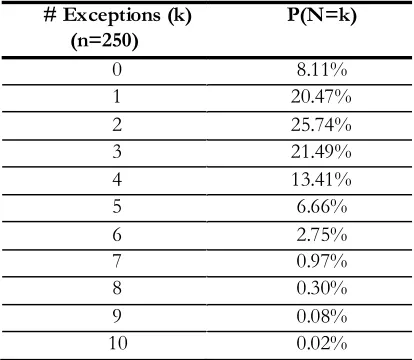
Since the test uses a 99% confidence level, the probability of an exception occurring during a given day is 1%. The P&Ls are assumed to be independent. So we can see the occurrence of exceptions at a given day as a Bernoulli experiment with a binomial distribution. We consider a model accurate if it generates an exception on 1% of the trading days.
We can calculate the probability that an accurate model generates exceptions in days using the properties of a binomial distribution:
26 MASTER THESIS EXTENDED ANALYSIS OF BACK TESTING FRAMEWORK Table 6.1 shows the probabilities for the accurate model.
# Exceptions (k)
Table 6.1 Exception probabilities accurate model
Test measurements
The input for the test consists of the number of exceptions that a model realised in 250 trading days. Based upon that result the test classifies the model in one of the three zones mentioned in Table 4.1.
Given the binomial distribution, we compute the expected number of exceptions during 250 days as:
(6.2)
Regulation formulates the null hypothesis of the test as probability of an exception occurring is equal to the expected probability of 0.01 . Or, if formulated in terms of probability:
(6.3)
The alternative hypothesis is probability of an exception occurring is significantly higher than the expected probability of 0.01 . This can put in a formula as:
(6.4)
Power
The Basel II back test has a small type 1 error. Recall that a type 1 error is rejecting the null hypothesis while it is true. So, a small type 1 error means that an accurate model is judged as inaccurate. Basel II rejects a model if it falls in the red zone. The red zone starts at 10 exceptions. The probability that an accurate model generates 10 or more exceptions is 0.03 %. This is the size of the type 1 error for the Basel II test.
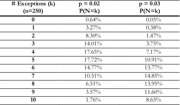
The Type 2 error concerns the acceptance of an erroneous model. This type 2 error corresponds to accepting the null hypothesis, while the alternative hypothesis is true. The Basel II back test suffers from type 2 errors. For example, suppose we have an inaccurate model with a 98% confidence level VaR or . This means that we have an expected number of exceptions generated in 250 trading days equal to:
MASTER THESIS EXTENDED ANALYSIS OF BACK TESTING FRAMEWORK 27 Since the Basel II back test checks if the model generates a 99% confidence level VaR, it should reject the null hypothesis, because the model has a probability p of 0.02 instead of the 0.01 under the null hypothesis. Table 6.2 shows what the probability of exceptions is, given that the tested model is inaccurate (having p values of 0.02 and 0.03 respectively). From the table we conclude that for the model with p of 0.02 the probability of an actual number of exceptions of four is 17.65% ( ). If we sum all the probabilities of the green zone, we can conclude that in 43.87% ( ) of all cases for the 0.02 and in 12.82%( ) for the p of 0.03 models, the test accepts the null hypothesis while it should reject it (type 2 error).
# Exceptions (k)
Table 6.2 Exception probabilities inaccurate models (p = 0.02 and p = 0.03)
The two problems we mentioned above make it impossible to set strict limits to model acceptation. This is the reason why Basel II regulation uses the 3-zone approach.
Size
The Basel II back test becomes more powerful if we increase the look back period. A small look back period and a high VaR confidence level will cause few exceptions. If the number of exceptions is small, the zones of Basel II are close together. So, the test will more easily classify a model in the wrong zone.
6.1.2
Kupiec Proportion of Failure Test
Description
Kupiec describes one of the first and best known back test alternatives (Kupiec, 1995). It is an extension of the
of exceptions. But this test judges a model as inaccurate if the number of exceptions is significantly higher or lower than the expected number. So the test is two tailed.
Goal
The goal of the Kupiec proportion of failure test is to determine if a VaR model is accurate by testing if the realised number of exceptions is not significantly different from the expected number of exceptions.
Exception Distribution
The distribution of the exceptions under the null hypothesis is the same as in the Basel II back test, the binomial distribution:
28 MASTER THESIS EXTENDED ANALYSIS OF BACK TESTING FRAMEWORK
Test measurements
The null hypothesis presumes that the empirically realised probability is equal to the theoretical probability :
(6.7)
The alternative hypothesis presumes that these probabilities are not equal:
(6.8)
Again, the test represents the exceptions by a random variable N with a binomial distribution. The most suitable test for comparing a theoretical and realised value is the likelihood ratio test. This type of test computes a test statistic for each number of realised exceptions. The following formula represents the test statistic:
(6.9)
The test statistic has a chi-square distribution with one degree of freedom
test statistic has a critical value. If the test statistic is bigger than this value, the actual number of exceptions is
Power
To give an impression of the power of the proportion of failure test, we determine the acceptance regions for a VaR models with 99% coverage level. This way we can compare the zone classification for this test with the one for the Basel II test. The acceptance region consists of the number of realised exceptions for which the test does not reject the null hypothesis, while the rejection region consists of the number of realised exceptions which the test rejects. We determine these zones by checking if the test statistic for a certain number of realised exceptions is larger than the critical value. The critical values have the chi square distribution with 1 degree of freedom. Finally we compute the acceptance region.
The main difference with the Basel II back test is the fact that the acceptance zone (green zone in Basel) does not start at zero exceptions. The Kupiec back test rejects a model if it generates too few exceptions. Next to that, the acceptance zone for 250 days of data with a 99% VaR is 1 6 (see Appendix B), where the green zone for Basel II is 0 4. But Basel II also has a yellow zone which ranges from 5 9 exceptions. So the Kupiec POF test rejects a model faster than the Basel II model. So it would suffer from less type 2, but more type 1 errors. Please note that the critical value we used for the Kupiec test is at 95% confidence level. But even for a 99% critical value the Kupiec test rejects models earlier than the Basel II back test.
Size
MASTER THESIS EXTENDED ANALYSIS OF BACK TESTING FRAMEWORK 29
6.1.3
Kupiec Time Until First Failure Test
Description
This test closely resembles the previous Kupiec test. The only difference is that the likelihood ratio test will now measure the time until the first exception.
Goal
The goal of this test is to test if the underlying VaR model is accurate by checking if the realised time until the first failure is significantly different from the expected time until the first failure.
Exception Distribution
Under the null hypothesis the exceptions have a binomial distribution:
(6.10)
Test measurements
If represents the time until the first exception, the test considers the following null hypothesis (if we use a 99% VaR level):
(6.11)
And the alternative hypothesis is:
(6.12)
The following formula now defines the test statistic as:
(6.13)
The chosen confidence level again determines the critical value of this test. Again, if the realised value of the test statistic is bigger than the critical value, the test judges the model as inaccurate.
Power
This test has lower power than the previous Kupiec test. This is caused by the fact that it only tests the period until the first occurrence of an exception.
Size
Since the underlying assumptions are the same as in the POF test, the sample size again needs to be large to provide powerful results.
6.1.4
Quality control of risk measures test
Description
30 MASTER THESIS EXTENDED ANALYSIS OF BACK TESTING FRAMEWORK
Goal
The goal of this method is to judge whether or not a VaR model is accurate in the same way Basel II does while controlling the type 2 error of Basel II.
Exception Distribution
The test uses the same assumptions as the Basel II method, so again the exceptions have a binomial distribution.
Test measurements
In essence, the quality control of risk measures test simply switches the hypotheses of the Basel II test. Let be the probability of an exception occurring during any given day. The hypotheses are defined as:
(6.14)
Hence if we accept the null hypothesis, we reject the VaR model. Inverting the hypotheses also switches the type 1 and type 2 errors of the Basel test. The test wants to control the type 2 error of the Basel II test, so it should control its own type 1 error. This error is rejecting the null hypothesis while it is true.
In Basel II the probability of rejecting an accurate model (99% VaR) is only 0.03% in case of a look back period of 250 days. This comes at a cost, because the probability that the test accepts (ending in the green zone) an inaccurate model is relatively large.
The confidence intervals in Basel II are such that the yellow zone starts at the point where the cumulative probability of the number of exceptions equals or exceeds 95%, and the red zone begins at the point where the cumulative probability equals or exceeds 99.99%.
The QCRM test computes the green, yellow and red zone classification while it makes sure that the type 1 error of their test does not become larger than 1%. De la Pena uses a numerical optimisation structure for this, which is described in Appendix E.1.
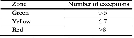
Table 6.3 shows the QCRM zone classification. The only difference is that they use a 99% limit to the red zone instead of the 99.99% limit used in Basel II.
Zone Number of exceptions
Green 0-5
Yellow 6-7
Red >8
Table 6.3 Zone classification (De la Pena, Rivera, Mata, 2007)
As we can see, the new test has a smaller yellow zone, compared to the Basel II back test So a 99% coverage VaR model will be accepted for 0-5, questioned for 6 or 7 and rejected for 8 or more exceptions.
Power
The designers of the QCRM test perform a formal power test to compare the quality of their test with the Basel II test. This shows that rejecting a 99% coverage VaR model while it is correct will happen in less than 0.03% of the cases for Basel II and in less than 0.4% of the cases for the QCRM test. So the QCRM test is a bit less powerful on this subject, but the probability of accepting an inaccurate model is reduced to (less than) 1%.
Size
This test does not suffer too much from size problems since its power is high.
6.2
Selection
MASTER THESIS EXTENDED ANALYSIS OF BACK TESTING FRAMEWORK 31
6.2.1
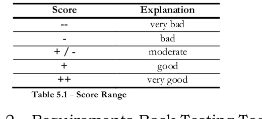
Score sheet
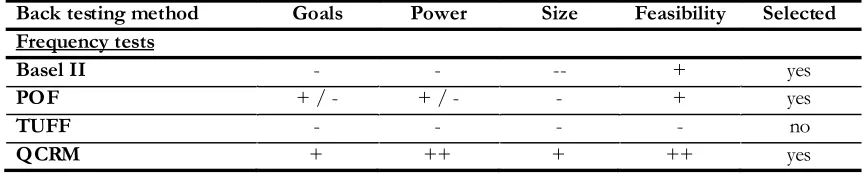
The following table contains the scores that we assigned to each of the requirements for the tests.
Back testing method Goals Power Size Feasibility Selected
Frequency tests
The Basel II test often accepts inaccurate models, so its power is not very high. It does not reach its goal very well, because of this power problem. But the tests feasibility is quite high since the test is the standard. We can also use it as a benchmark for the other tests in the process. Next to that, it is quite easy to implement. So, we select the Basel II test.
Kupiec Power Of Failure (POF)
The POF test reaches its goal reasonably well. It has a small acceptance region compared to Basel II and it can provide more insight if a model is over- or underestimating risk.
The power of the POF test cannot be directly compared to the power of the Basel II model. Since a likelihood ratio statistic is used, it is not possible to compute the type 1 and 2 errors. The probability distribution of the number of exceptions as given in Appendix B is not cumulative. All the test can do is either accept or reject the accuracy of a model at a given confidence level. But, the acceptance region for Kupiec is smaller than the Basel II back test, so its power score is better than for the Basel II back test. The same reasoning holds for the size score.
The feasibility of this test is moderate. It is easy to implement and tests the number of exceptions in a slightly different way and stricter compared to the Basel II test, which might provide additional insight. The most interesting feature of this test is its ability to detect VaR models that overestimate risk or produce too few exceptions. If this happens, the Basel II capital requirement is low, since no or few exceptions are produced by the model.
So, we select the POF test.
Kupiec Time Until First Failure (TUFF)
The goal of TUFF is to test VaR model accuracy by judging the time until first failure. The likelihood ratio test reaches this goal fairly well.
The power of the test is low, compared to the POF test, since it only tests for the time until the first exception occurs and does not look at the remainder of the period.
The size receives the same score as the POF test since the underlying assumptions are the same as in the POF test, so the sample size again needs to be large provide powerful results.
The added value of the test lies in the time until the first failure property. But it tests only for the first failure and does not say anything about the distribution of exceptions over time. This does not provide much insight in VaR model accuracy.
So, we do not select the TUFF test.
QCRM
32 MASTER THESIS EXTENDED ANALYSIS OF BACK TESTING FRAMEWORK
the costs for reaching these results are limited. The QCRM test has a slightly increased error on rejecting accurate models compared to the Basel II back test.
Since the power of the test increased, the influence of the sample size is also less important. For lower sample sizes, the QCRM test will have better results compared to Basel II, since its zone classification is stricter.
6.3
Implementation
One of the requirements of the tool states that we should present the test results for each back testing method with a zone classification similar to the Basel II back test. The QCRM back test also uses a zone classification which is described in section 6.1.4. The following section describes how this classification is implemented for Kupiec test.
6.3.1
Zone Classifications Kupiec
In order to make the results of this test easy to interpret, we introduce a zone classification similar to the Basel II back test. The green, yellow and red zones again have the same interpretation as in the Basel II back test. Next to that, we introduce two new zones (dark blue and light blue) that have a similar interpretation as the yellow and red zone. But where the yellow and red zones indicate that the model is possibly inaccurate in that it generates too many outliers, the dark and light blue zones indicate that the model is possibly inaccurate because it generates too few outliers. In order to give an idea what the Kupiec zone classification looks like we determine the zone classification for a 99% VaR level and a look back period of 250 days.
Zone Number of exceptions
Dark blue 0
Light blue 1
Green 2-5
Yellow 6
Red
Table 6.5 Zone classification Kupiec test
So if such a model generates 0 or 1 exceptions the Kupiec test indicates that the model overestimates risk. If it generates
2-exceptions. If the number of realised exceptions is 7 or larger, the Kupiec test indicates that the model underestimates risk.
34 MASTER THESIS EXTENDED ANALYSIS OF BACK TESTING FRAMEWORK
7
E
XCEPTION
C
LUSTERING
A disadvantage of testing exception frequency concerns the independence of exceptions over time. Consider the example of the introduction of Chapter 6 again: if the number of exceptions over the 250 days is 4, the exception frequency test will judge the VaR model as accurate. But if all four exceptions were during the last 20 days, it is likely there is some market condition that the VaR model cannot cope with: hence the model is inaccurate. On top of that, if clustering of exceptions happens at multiple banks at the same time, this can have large consequences for the industry. In this situation, the independence test proves its usefulness. In an accurate VaR model, the exceptions should be independent of each other. In other words, the probability that an exception occurs during a given day should be independent of the history of exceptions before that day. The independence tests consider this property of the exceptions. This type of test only considers the occurrence of the exceptions over time. The tests do not consider the number of exceptions or the size of the exceptions.
This chapter gives an overview of the exception frequency tests that we discuss in this project. The first section describes the details about the methods we encountered during the literature research. The second section contains the selection of the methods that we implement in the tool. The third section describes what choices we made in the implementation of the tests. Finally, the fourth section gives an overview of the results of the initial test run.
7.1
Test Descriptions
In this section we describe the exception clustering tests we investigated in the literature research. For each back test we first give a general description of the test. The goal is one of the requirements that we use in the test selection. Next, we indicate what the underlying distribution of the exceptions is. After that we indicate what the
errors are. Large errors mean low power of the test. Finally, we describe what the influence of the length of the look back period on the test results is.
7.1.1
Likelihood Ratio Test for Independence
Description
The likelihood ratio test for independence is an addition to the exception frequency tests by testing if no clustering of exceptions over time occurs. (Christoffersen, 1998)
Goal
The independence test checks the accuracy of the VaR model by investigating if the occurrence of exceptions over time is independently distributed.
Exception Distribution
The basic assumption of the test is that an accurate VaR model will generate an independent series of exceptions. This is reasonable since an accurate VaR model should generate an exception on any given day with a probability p. It does not depend on the results of previous days.
The following formula represents the series of results showing if exceptions occurred or not.
(7.1)
MASTER THESIS EXTENDED ANALYSIS OF BACK TESTING FRAMEWORK 35 . He wants to proof this by showing that the sequence of results is independently Bernoulli distributed with parameter p (= probability of an exception on a single day).
Test measurements
Christoffersen describes a test that is capable of testing independence using a first order Markov chain for two successive results. The transition probability matrix shows what the probabilities are of either an exception or no exception given that the day before an exception or no exception has taken place:
(7.2)
Here is the probability that occurs at time given that occurred at time . The following formula shows the likelihood function for this function:
(7.3)
Here is the number of observations with value followed by . We estimate the Markov transition matrix by simply computing the ratios of the appropriate cells (which are the maximum likelihood estimates for the values in matrix (7.2)):
(7.4)
In the next step, we take a look at the result vector . If the elements of the result vector are independent, the Markov transition probability should look like:
(7.5)
In other words, there is no difference between the probabilities for an exception or no exception for a certain day, no matter what the result was on the day before. Hence we define the null hypothesis as:
(7.6)
The maximum likelihood estimator for is:
(7.7)
We compute the likelihood function under the null hypothesis by:
(7.8)
Finally, we compute the test statistic by the following formula:
36 MASTER THESIS EXTENDED ANALYSIS OF BACK TESTING FRAMEWORK
We obtain the formulas for the maximum likelihood estimates for and by filling in the maximum likelihood estimates that we saw in formulas (7.4) and (7.7). The test has an asymptotically distribution.
Power
We do not compare the power of the likelihood ratio test for independence to the power of the exception frequency tests. The reason for this is that the methods test completely different properties of the VaR model. We showed in the introduction to the back testing types, that the change of one property does not influence the back test of the other property. So it is not useful to compare the power of these tests. But Christoffersen uses Monte Carlo simulations to test how often his method rejects an inaccurate model. He concludes that the test has problems with rejecting inaccurate models for smaller sample sizes.
Size
This exception independence test does not perform very well if the number of exceptions is