DOI: 10.1534/genetics.105.045781
Improvement of Mapping Accuracy by Unifying Linkage and
Association Analysis
Xiang-Yang Lou,* Jennie Z. Ma,
†Mark C. K. Yang,
‡Jun Zhu,
§Peng-Yuan Liu,**
Hong-Wen Deng,** Robert C. Elston
††and Ming D. Li*
,1*Department of Psychiatric Medicine, University of Virginia, Charlottesville, Virginia 22911,†Department of Psychiatry, University of Texas Health Science Center, San Antonio, Texas 78229,‡Department of Statistics, University of Florida, Gainesville,
Florida 32611,§Department of Agronomy, Zhejiang University, Hangzhou, Zhejiang 310029, People’s Republic of China, **Osteoporosis Research Center, Creighton University Medical Center, Omaha, Nebraska 68131 and††Department of
Epidemiology and Biostatistics, Case Western Reserve University, Cleveland, Ohio 44109 Manuscript received May 17, 2005
Accepted for publication September 14, 2005
ABSTRACT
It is well known that pedigree/family data record information on the coexistence in founder haplotypes of alleles at nearby loci and the cotransmission from parent to offspring that reveal different, but complementary, profiles of the genetic architecture. Either conventional linkage analysis that assumes linkage equilibrium or family-based association tests (FBATs) capture only partial information, leading to inefficiency. For example, FBATs will fail to detect even very tight linkage in the case where no allelic association exists, while a violation of the assumption of linkage equilibrium will result in biased estimation and reduced efficiency in linkage mapping. In this article, by using a data augmentation technique and the EM algorithm, we propose a likelihood-based approach that embeds both linkage and association analyses into a unified framework for general pedigree data. Relative to either linkage or association analysis, the proposed approach is expected to have greater estimation accuracy and power. Monte Carlo simulations support our theoretical expectations and demonstrate that our new methodology: (1) is more powerful than either FBATs or classic linkage analysis; (2) can unbiasedly estimate genetic parameters regardless of whether association exists, thus remedying the bias and less precision of traditional linkage analysis in the presence of association; and (3) is capable of identifying tight linkage alone. The new approach also holds the theoretical advantage that it can extract statistical information to the maximum extent and thereby improve mapping accuracy and power because it integrates multilocus population-based association study and pedigree-based linkage analysis into a coherent framework. Furthermore, our method is numerically stable and computationally efficient, as compared to existing parametric methods that use the simplex algorithm or Newton-type methods to maximize high-order multidimensional likelihood functions, and also offers the computation of Fisher’s information matrix. Finally, we apply our methodology to a genetic study on bone mineral density (BMD) for the vitamin D receptor (VDR) gene and find that VDR is significantly linked to BMD at the one-third region of the wrist.
T
WO approaches are commonly used in pedigree-or family-based gene mapping, i.e., linkage anal-ysis (e.g., Elston and Stewart 1971; Haseman and Elston 1972; Ott 1974; Lander and Green 1987; Risch 1990; Ward 1993; Amos 1994; Kruglyak and Lander1995; O’Connelland Weeks1995; Kruglyak et al.1996; Gudbjartssonet al.2000; Abecasiset al.2002) and family-based association tests (FBATs) (e.g., Falkand Rubinstein1987; Spielmanet al.1993; Lazzeroniand Lange1998; Lairdet al.2000; Rabinowitzand Laird 2000). Linkage analysis focuses on gene cosegregation that can be characterized by inheritance vectors or gene concordance between related individuals (identical-by-descent, IBD, or identical-in-state, IIS) at each locus, while association tests (which, when due to linkage, are tests of gametic association, also called linkage disequilibrium,LD) directly utilize allele status and linkage phase that record historic events. Pedigree data contain both these components of information that give rise to comple-mentary profiles of the genetic architecture. Either link-age or association analysis alone, however, can capitalize only on the genetic information from one of these components and fails to grasp the whole picture, thereby leading to a loss in mapping accuracy and statistical power. To illustrate the limitations of applying either a link-age or association approach alone, let us consider the affected sib pair design used in Risch(1990) and Risch and Merikangas(1996). First, traditional linkage anal-ysis will give a biased result in the presence of popula-tion associapopula-tion. To simplify our exposipopula-tion, assume there are a diallelic disease locusQwith allelesQandq and a codominant marker locusAwith allelesAanda. Alleles Q and A have the same frequency and are in perfect association, and letpQ¼pA¼pAQ¼p. Table 1 lists the assumed probabilities (under no association), 1Corresponding author: 1670 Discovery Dr., Ste. 110, Charlottesville,
VA 22911. E-mail: [email protected]
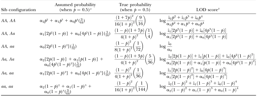
the true probabilities, and Risch’s (1990) LOD scores of all six possible sib configurations in the case where markerAis unlinked to a recessively inherited disease gene Q. Using Risch’s (1990) EM iterative Equation 4, we can obtain the maximum-likelihood estimates (MLEs) of the posterior probabilities that the affected sib pairs share i marker alleles IBD (i ¼ 0, 1, 2). To illustrate the result, we takepto be a specific value, say p¼0.5, then we have^z2 ¼0:444,^z2 ¼0:487, and^z0 ¼
0:069, respectively, and the expected LOD (ELOD) ¼ 0.384. These values deviate substantially from the true IBD sharing scores of 0.25, 0.5, and 0.25, respectively, and exhibit a spuriously excessive allele sharing. This suggests that a false-positive result can occur in allele-sharing anal-ysis. We further demonstrate that, generally, the assumed likelihood is a monotonically decreasing function of the recombination fraction u for u 2 [0, 0.5] (see the appendix). This means that, if the true recombination
fractionu06¼0, we may still obtain an estimate of zero. Second, neglecting to take account of information on association may cause loss of statistical power. As pointed out by Rischand Merikangas(1996), the allele-sharing method is much less powerful than the transmission/ disequilibrium test (TDT) method in the cases they considered,i.e., when there is no recombination and the alleles at the two loci are perfectly associated. This arises because the linkage statistic, the mean allele sharing, fails to consider theallele-specificIBD sharing. Actually, alleleA(increasing disease risk) contributes more allele sharing to the statistic, whereas alleleacontributes less, so that the overall mean allele sharing is diluted. Our simulations of model-based linkage-only analysis sup-port this theoretical argument,i.e., the plausible bias and the reduced power (seesimulation studies).
Because they fail to incorporate information on link-age, FBATs are inherently conservative, and so they can-not detect linkage even when two or more siblings are available, unless there is also population association. The conclusion by Rischand Merikangas(1996) was drawn from the ideal circumstance where the marker is the disease gene itself. In such a situation, FBATs reach their maximum potential power. In practice, however, it may not be true that a marker happens to have the same variant frequencies as, and be perfectly associated with, the disease gene of interest, even for fine mapping, as there are always many polymorphic SNPs within a gene whereas only a few may be responsible for the change of its function. Both theoretical and empirical studies (e.g., Kruglyak 1999; Hinds et al. 2005) have shown that the founder LD within a small region has usually been largely disrupted by various population forces, such as recombination, gene conversion, and/or mutation ac-cumulated over time, so that high-LD regions with little genetic shuffling, termed haplotype blocks, span only a very short distance, implying that strong LD is not inevitable with tightly linked loci. HapMap studies also indicate that the frequencies of variants change from one SNP to another largely within a block (I nterna-tional HapMap Consortium 2003). In practical
ap-plication, FBATs can therefore lose their theoretical power even with closely linked loci, owing to the violation of such an ideal assumption. Furthermore, association may extend over a great distance, even to nonsyntenic loci because of factors other than linkage, such as pop-ulation subdivision and admixture, poppop-ulation bottle-necks, mutation, gene conversion, meiotic drive, sampling or ascertainment bias, nonrandom mating, and coan-cestry. Caution is also required in that a positive result TABLE 1
Probabilities and RISCH’s (1990) LOD scores in affected sib-pairs designs for a marker unlinked to, but perfectly associated with,
a recessive disease gene
Sib configuration
Assumed probability (whenp¼0.5)a
True probability
(whenp¼0.5) LOD scoreb
AA,AA a2p21a1p31a0p4(649)
ð117pÞ2 16ð11pÞ2
9
16 log
^z2p21^z1p31^z0p4
a2p21a1p31a0p4
AA,Aa a1[2p2(1 –p)]1a0[4p3(1 –p)](163)
ð1pÞð117pÞ 4ð11pÞ2
1
4 log
^
z1½2p2ð1pÞ1^z0½4p3ð1pÞ
a1½2p2ð1pÞ1a0½4p3ð1pÞ
AA,aa a0[2p2(1 –p)2](1 32)
ð1pÞ2 8ð11pÞ2
1
72 log
^z0
a0
Aa,Aa a2[2p(1 –p)]1a1[p(1 –p)]1
a0[4p2(1 –p)2](165)
ð1pÞð113pÞ 4ð11pÞ2
5 36 log
^z2½2pð1pÞ1^z1½pð1pÞ1^z0½4p2ð1pÞ 2
a2½2pð1pÞ1a1½pð1pÞ1a0½4p2ð1pÞ2
Aa,aa a1[2p(1 –p)2]1a
0[4p(1 –p)3](163)
ð1pÞ2 4ð11pÞ2
1
36 log
^
z1½2pð1pÞ 2
1^z0½4pð1pÞ 3
a1½2pð1pÞ2
1a0½4pð1pÞ3
aa,aa a2(1 –p)21a1(1 –p)31
a0(1 –p)4(649)
ð1pÞ2 16ð11pÞ2
1 144
log ^z2ð1pÞ 2
1^z1ð1pÞ3
1^z0ð1pÞ4
a2ð1pÞ21a1ð
1pÞ31a0ð 1pÞ4
aa
i(i¼0, 1, 2) is the prior probability that two siblings shareialleles IBD,a2¼a0¼0.25,a1¼0.5, respectively.
b^z
from an FBAT does not necessarily imply the presence of tight linkage;i.e., an FBAT alone cannot distinguish strong association and loose linkage from weak associ-ation and tight linkage (Elston1998; Whittakeret al. 2000).
Therefore, it is of great interest to remedy the above limitations. A judicious way is to take both these pieces of information into consideration in gene mapping. Such an idea was conceived in earlier literature (e.g., MacLean et al.1984) and adopted in some computer software such as LINKAGE (Lathrop and Lalouel 1984; Lathrop et al.1985). Unfortunately, the bonus from joint mapping was not recognized, so this remarkable idea has been buried for several years (Xiongand Jin2000). Recently, Zhaoet al.(1998) proposed a semiparametric method for a combined linkage and linkage disequilibrium analysis. Xiong and Jin (2000) advocated a likelihood-based parametric method for joint analysis with nuclear family data. Cantoret al.(2005) further extended Xiongand Jin’s (2000) method for general pedigrees. Liet al.(2005) suggested an approach that identifies associated and potentially causal SNPs through joint modeling of link-age and association. Parallel to parametric ones, variance components (e.g., Allisonet al. 1999; Fulkeret al. 1999; Abecasiset al. 2000) and nonparametric (Huang and Jiang 1999; Wicks 2000; Wicks and Wilson 2000; Lazzeroni 2002) methods have also been developed. However, those methods work mostly for specific data structures and types such as affected sib pairs, nuclear families, and categorical traits and/or can provide a solution only for specific problems such as single-point analysis. The bonus of combined mapping has also not been thoroughly explored. By invoking a data augmen-tation technique and the EM algorithm, we have evolved a general likelihood-based statistical framework for inte-grating linkage and association analyses (Louet al.2005). In the present article, we further extend this model-based approach for general pedigrees. This approach allows us to simultaneously perform segregation, linkage, and asso-ciation analyses, i.e., to estimate penetrance functions, genetic distances, and association parameters, as well as to carry out the corresponding hypothesis tests within a unified framework. More appealingly, it adds several unique strengths to existing parametric methods (e.g., Xiongand Jin2000; Cantoret al.2005; Liet al.2005). First, this framework is conceptually straightforward, flex-ible, easy to generalize, and also comprehensive, so that it covers a wide range of cases with multiple loci and/or multiple alleles. Multilocus mapping and epistatic QTL mapping can be implemented as well under the same concept. Second, our new approach is computationally efficient and powerful. We formulated the closed-form solutions for MLEs implemented with EM iteration and thus avoid the computational difficulty of high-order multidimensional searches, leading to less computational time per iteration and quick convergence. Third, due to the advantage of the EM algorithm over the simplex
algorithm and Newton-type methods in the context of a mapping study, as pointed out by some authors (e.g., Landerand Green1987), our new approach is numer-ically stable, as compared with existing methods. In our experience, a wide range of initial values appears to give good convergence. Finally, we offer the computation of Fisher’s information matrix and hence can provide the estimation precision of MLEs. Although this article em-phasizes a demonstration of the improvement in mapping accuracy using a two-locus model,i.e., one marker and one trait gene, we use an interval mapping model to describe our new approach in themodel and methodsection for readers to have a clearer picture about it. After presenting the theory, we use simulation studies to compare the power of an FBAT, of the pure linkage method, and of our new approach and the estimation precision of the latter two. An application to the genetic study of bone mineral density (BMD) is used to demonstrate this new methodology. Finally, we discuss some relevant issues to provide further insights into this approach.
MODEL AND METHOD
Here we use a three-diallelic-locus model to illustrate the approach. Suppose there are three loci, one trait gene or QTL,Q, bracketed by a pair of flanking mark-ers,AandB, respectively. LetA,a,Q,q,B, andbbe the alleles at the three loci, respectively. All the alleles to-gether form eighthaplotypes,AQB,AQb,AqB,Aqb,aQB, aQb,aqB, andaqb. These haplotypes unite to generate a total of 36diplotypes,AQB/AQB,AQB/AQb,. . ., andaqb/ aqb, where the ‘‘/’’ denotes the separation of the ma-ternally and pama-ternally derived gametes. The 36 diplo-types are collapsed into 27zygote genotypes, each with an identical allelic combination at all the loci, and further, into 9 marker genotypes and 3 QTL genotypes. Owing to the fact that genotypes areconflated datathat ignore the linkage phases of diplotypes, some of the genotypes consist of .1 diplotype. For example, all 4 diplotypes AQB/aqb,AQb/aqB,AqB/aQb, andAqb/aQBexhibit the same genotype, AaQqBb. To express the relationship between diplotypes and genotypes, we denote by GðÞ, GmðÞ, andGqðÞthe many–one mapping operators
tak-ing the genotypes at all loci, the marker loci and the QTL, of a diplotype in parentheses, respectively. Thus, GðAQB=aqbÞ¼GðAQb=aqBÞ¼ GðAqB=aQbÞ¼GðAqb=aQBÞ ¼
AaQqBb;GmðAQB=aqbÞ ¼ GmðAQb=aqBÞ¼ GmðAqB=aQbÞ¼
GmðAqb=aQBÞ ¼AaBb, and GqðAQB=aqbÞ ¼ GqðAQb=
aqBÞ ¼ GqðAqB=aQbÞ ¼ GqðAqb=aQBÞ ¼Qq.
We usepAQB,pAQb,. . .,paqbandPAQB/AQB,PAQB/AQb,. . ., Paqb/aqbto denote the frequencies of the haplotypesAQB, AQb,. . .,aqband diplotypesAQB/AQB,AQB/AQb,. . ., aqb/aqb, respectively, in the population studied. If the population is at Hardy–Weinberg equilibrium, we have
The frequencies of the haplotypes can be decomposed into different components determined by the allele fre-quencies at each locus and LD coefficients of different orders;e.g.,
pAQB ¼pApBpQ1pADBQ1pBDAQ1pQDAB1DAQB;
wherepA,pB, andpQare the frequencies of allelesA,B, andQ, respectively andDAQ,DBQ,DAB, andDAQBare the LD coefficients, respectively. Reversely, the frequencies of alleles and LD coefficients can also be represented by the frequencies of haplotypes;e.g.,pA¼pAQB1pAQb1pAqB1 pAqb,. . .,DAB ¼ pAB pApB,. . ., and DAQB ¼ pAQB
pADBQpBDAQpQDABpApBpQ. For a more general expression with an arbitrary number of alleles and/or loci, see one of our recent communications (Lou et al. 2003) for details.
Crossing overbetween a pair of contiguous loci may take place during meiosis. Either recombination (R) or non-recombination (N) between each of the pairs of adjacent loci (i.e., A and Q, B and Q) will give rise to four re-combination configurations described byNN,NR,RN, or RR. The frequency of a new haplotype is a function of the recombination fraction(s) associated with its recombina-tion configurarecombina-tion(s). For simplicity, we here ignore cross-over interference during gametogenesis. LetuAQanduBQ
be the recombination fractions between lociAandQand betweenBandQ, respectively. The frequencies of these four configurations can be expressed in terms ofuAQand
uBQ,i.e., (1uAQ)(1uBQ), (1uAQ)uBQ,uAQ(1uBQ), or uAQuBQ corresponding to NN, NR, RN, or RR, re-spectively. Furthermore, the conditional probability of a zygote randomly formed by the haplotypes generated from a pair of parents is a product of the frequencies of paternally and maternally original haplotypes.
For any complex trait, either continuous or discrete, there is no one–one correspondence between genotype and phenotype. The conditional probability of observ-ing a phenotype given a specified genotype, termed the penetrance function, is thus used to characterize the rela-tionship between genotype and phenotype. Because the phenotype is genetically determined by the genotypes at locusQ, the penetrance function, given diplotype D, can be expressed as
fðyjDÞ ¼fðyjGqðDÞÞ ¼ 1 ffiffiffiffiffiffi 2p
p
sexp
ðymG
qðDÞÞ
2
2s2
" #
;
for a continuous phenotype in which it is typically assumed that the distribution within each subpopulation defined by genotype is normal, wheremG
qðDÞis the genotypic mean of
QTL genotype GqðDÞð¼QQ;Qq;or qqÞ and s2 is the
residual variance. For a categorical trait the penetrance fðyjGqðDÞÞis defined as the probability that individuals
with genotypeGqðDÞmanifest phenotypey. We may specify
different penetrance functions to mothers, fathers, and children on the basis of the inheritance pattern of the trait under investigation. To make this presentation terser, here
we assume the same penetrance for the parental and off-spring generations. However, it is not difficult to recast the methodology to be applicable to the case with different penetrance functions. Mendelian trait(s) and marker(s) can be viewed as specific examples with full penetrance. Then the methodology developed hereinafter is also ap-plicable to their analysis.
In a gene-mapping study aimed at estimating param-eters of penetrance, association, and position (usually measured by the recombination fractions), a major chal-lenge is thatlatent dataexist, also referred to asmissing data, that cannot be directly observed, such as disease genotype, diplotype, and recombination configuration. We hypothesize the observed data, i.e., marker geno-types and phenogeno-types, together with the latent data,i.e., diplotypes and recombination configurations, as com-plete data, also termedaugmented data. Correspondingly, the observed data alone are calledincomplete data. The observed data can be viewed as mixtures of complete data and then we can use a mixture model to tackle the issue of parameter estimation.
The complete data likelihood: Denote marker, dip-lotype/haplotype, recombination configuration, and phe-notype data byM,D/H,R, andy, respectively. Observed marker and phenotypic data are in boldface type while the missing data for parent and child diplotypes and child recombination configurations are in script type. We first use nuclear family data, in which there is no phenotypic covariance between parents and children, to demonstrate parameter estimation within a unified frame-work of interval mapping and LD mapping, and then extend the method to general pedigree data.
With N unrelated nuclear families randomly drawn from a general population, the overall likelihood is the product of individual family likelihoods, denoted L1,
L2,. . .,LN. Let us present an example to demonstrate
how to build the likelihood function. In the example, familyiconsists of a mother with diplotypeAQB/AQB (Dm
i ) and phenotypeyi
m, a father withAQB/Aqb (Df
i) andyif, and two children with diplotypes and recombi-nation configurationsAQB/AQBandNN/RN(Do
i1;Ri1)
andAQB/AQbandNN/NR(Do
i2;Ri2), respectively, and
phenotypesyo
i1andyoi2, respectively. The likelihood can
be expressed by a three-level hierarchical model,
Li¼Lðymi ;y f i;y
o
i1; yio2;Dmi ;D f i;D
o
i1;Ri1;Dio2;Ri2jVÞ
}PrðDm i ÞPrðD
f iÞfðy
m i jD
m i Þfðy
f ijD
f iÞ
3Y
2
j¼1
PrðDo
ij;RijjDmi ;D f iÞfðy
o ijjD
o ijÞ
h i
}pAQB3 pAqbuAQð1uAQÞ3uBQð1uBQÞ3
3fðymi jQQÞfðyfijQqÞfðyio1jQQÞfðyoi2jQQÞ;
(e.g., genotypic values and the residual variance,VQ), and position parameters (recombination fractions,
VR), related to the parental diplotype distribution, the phenotype density functions, and PrðDo
ij;RijjDmi ;D
f
iÞ, respectively. PrðDo
ij;RijjDmi ;D
f
iÞ represents the condi-tional probability of childjof familyihaving diplotype Do
ijand recombination configurationRijgiven parental diplotypes Dm
i and D
f
i. The overall likelihood can be represented as
Lðym;yf;yo;Dm;Df;Do;RjVÞ
¼Y
N
i¼1
Li}
YN
i¼1
PrðDm
i ÞPrðDfiÞfðymi jDmi ÞfðyfijDfiÞ
3QNi
j¼1 PrðDoij;RijjDmi ;DfiÞfðyoijjDoijÞ
h i 8 < : 9 = ;
}pnAQB
AQBp nAQb
AQb . . .p naqb
aqbu nuAQ
AQ ð1uAQÞ nu¯AQunuBQ
BQ ð1uBQÞ nu¯BQ
3Y
N
i¼1
fðyimjDm
i ÞfðyfijDfiÞ
YNi
j¼1
fðyoijjDo ijÞ
" #
; ð1Þ
where the y’s are the phenotypic vectors; D’s are the diplotype vectors;Ris the recombination configuration for the children;Niis the number of children within family i;nAQB,nAQb,. . .,naqbare the numbers of haplotypesAQB, AQb,. . ., aqb appearing in parental diplotypes, respec-tively;nuAQandn¯uAQare the numbers of recombinants and
nonrecombinants between lociAand Qexisting in the recombination configurations, respectively; andnuBQ and
nu¯BQ are those betweenBandQ, respectively.
In many cases, information is partial because of experi-mental errors, financial limitations, or other practical constraints, as often occurs in studies of late-onset dis-eases such as Alzheimer’s disease where parents are unavailable. Since missing phenotypic observations can be treated by simply setting the correspondingf(yjD)’s equal to 1 wherever they occur in the above likelihood, Equation 1 automatically covers the likelihoods of fam-ily data with missing phenotypes like TDT-type data. For data with missing diplotypes such as sibship data, in-stead of Equation 1 we can use a form of mixture model summing over all plausible diplotypes and/or recombi-nation configurations compatible with the available data to represent such likelihoods and so address the statistical analysis within the EM framework described in The incomplete data likelihoodsection.
Equation 1 can be generalized to the case ofNpedigrees,
LðyF;yN;DF;DN;RjVÞ ¼Y N
i¼1
Li}p nAQB
AQBp nAQb
AQb . . .p naqb
aqb
3unuAQ
AQ ð1uAQÞ n¯uAQ
3unuBQ
BQ ð1uBQÞ nu¯BQ
3 Y
N
i¼1
QNF
i
j¼1fðyFijjDFijÞ
3 QNiN
j¼1fðyijNjD N ijÞ 2 4 3 5;
ð19Þ
where the likelihood of pedigreei,
Li¼
YNF
i
j¼1 PrðDF
ijÞfðy
F
ijjD
F
ijÞ
h i YNN
i
j¼1 PrðDN
ij;RijjDmij;D
f
ijÞfðy
N ijjD N ijÞ h i ¼ Y NF
i1N
N
i
j¼1
PrðDijÆ;RijjæÞfðyijjDijÞ
h i
;
assuming that the rightmost is ordered as Elstonand Stewart’s (1971) recursive form in which PrðDij;ÆRijjæÞ represents the probability of either childjgiven the par-ental diplotypes or founderjwithin pedigreei;Dm
ij and
Df
ij are the parental diplotypes of nonfounderjwithin pedigreei, respectively;yFandyNare the founder and non-founder phenotypic vectors;DF
andDN
are the founder and nonfounder diplotype vectors;Ris the recombina-tion configurarecombina-tion for nonfounders, respectively;NiFand NiNare the numbers of founder(s) and nonfounder(s) within pedigreei;nAQB,nAQb,. . .,naqbare the numbers of haplotypesAQB,AQb,. . .,aqbappearing in founder diplotypes, respectively; andnuAQ,n¯uAQ;nuBQ, andnu¯BQ are
the numbers of recombinants and nonrecombinants be-tween lociAandQand betweenBandQacross allN pedigrees, respectively.
The maximum-likelihood estimator can be derived through differentiating the log-likelihood with respect to V and then setting each derivative equal to 0 and solving the set of simultaneous equations. Define the identity indicators
IðQQjDÞ ¼
1 ifGqðDÞ ¼QQ;
i:e:;diplotypeDis compatible with
the genotypeQQ
0 otherwise; 8 > > > > > < > > > > > :
IðQqjDÞ ¼ 1 ifGqðDÞ ¼Qq
0 otherwise; (
and
IðqqjDÞ ¼ 1 ifGqðDÞ ¼qq
0 otherwise: (
The MLEs for the likelihood (1) are
^
pAQB¼nAQB 4N ; ^pAQb¼
nAQb
4N; . . .; ^paqb¼ naqb
4N;
ˆ uAQ¼
nuAQ
nuAQ1n¯uAQ
; ˆuBQ¼ nuBQ
nuBQ1n¯uBQ
;
ˆ mG¼
PN i¼1 IðGjD
m i Þy
m i 1IðGjD
f iÞy
f i1
PNi
j¼1IðGjDoijÞy o ij
h i
PN
i¼1 IðGjDmi Þ1IðGjDfiÞ1
PNi
j¼1IðGjDoijÞ
h i ;
ˆ s2¼
PN
i¼1 ðyimmˆGqðDmiÞÞ
21ðyf
imˆGqðDfiÞÞ
21PNi
j¼1ðyoijmˆGqðDoijÞÞ
2
h i
2N1PN i¼1Ni
;
ð2Þ
^
fðyjGÞ ¼ X
N
i¼1
X0
0 IðGjDm
iÞIðy¼ymiÞ1IðGjDfiÞIðy¼yfiÞ
"
1X
Ni
j¼1 IðGjDo
ijÞIðy¼y
o
ijÞ
#! XN
i¼1
X0
0 IðGjDm
iÞ
"
1IðGjDf
iÞ1
XNi
j¼1 IðGjDo
ijÞ
#!
;
for categorical traits, whereG2 fQQ,Qq,qqg; and in-dicatorsI(y¼yim),I(y¼yif), andI(y¼yijo) are 1 wheny¼ yim,y¼yif, andy¼yijo, respectively, and 0 otherwise. The MLEs of the recombination parameters for likelihood (19) are the same as those for likelihood (1), and the other MLEs have similar forms,
^ pAQB¼
nAQB
2PN i¼1NiF
; ^pAQb¼ nAQb
2PN i¼1NiF
; . . . ; ^paqb¼ naqb
2PN i¼1NiF
;
ˆ
mG¼
PN i¼1
PNF
i
j¼1IðGjDFijÞyFij1
PNN
i
j¼1IðGjDNijÞyijN
h i
PN i¼1
PNF
i
j¼1IðGjDFijÞ1
PNN
i
j¼1IðGjDNijÞ
h i ;
ˆ
s2¼
PN i¼1
PNF
i
j¼1ðyijFmˆGqðDFijÞÞ
21PNN
i
j¼1ðyNij mˆGqðDNijÞÞ
2
h i
PN
i¼1ðNiF1N N i Þ
;
ð29Þ
for quantitative traits, and
^ fðyjGÞ ¼
PN i¼1
PNF
i
j¼1IðGjDFijÞIðy¼yFijÞ1
PNN
i
j¼1IðGjDNijÞIðy¼yNijÞ
h i
PN i¼1
PNF
i
j¼1IðGjDFijÞ1
PNN
i
j¼1IðGjDNijÞ
h i ;
for category traits.
Unlike the traditional approach, for flexibility we make here no assumption such as that the recombina-tion fracrecombina-tion between the two markers can be known a priori. If the recombination fraction between the two markers (uAB) is available, however, the corresponding terms with respect to one of the recombination frac-tions,uAQanduBQ, will disappear from the above esti-mation procedure since any one of the two is a function of the other one and ofuAB. A grid search procedure can also be used for estimating QTL position on the basis of the preceding methodology.
The incomplete data likelihood: In practice, only marker genotype and phenotype data are observed, whereas the data on diplotypes, recombination events, and QTL genotypes are hidden. The observed data are mixtures of component complete data, and the statistical analysis becomes a typical mixture issue. Let us go back to the above example again and assume that only marker genotypes AABB (Mim), AABb (Mif), AABB (Mo
i1), and
AABb(Mo
i2) and phenotypesy m
i ;y
f
i;y
o
i1, andy o
i2are
avail-able for the mother, father, and two children of familyi, respectively. NowMm
i is a mixture of diplotypesAQB/ AQB,AQB/AqB, andAqB/AqB; andMifis composed of diplotypesAQB/AQb,AQB/Aqb,AQb/AqB, andAqB/Aqb; and bothMo
i1 andM o
i2also consist of unidentified
dip-lotype(s) together with recombination configuration(s) nested within the paired parental diplotypes. The likeli-hood can be formulated as
Li¼Lðymi ;y
f
i;y
o
i1;y o
i2;M m
i ;M
f
i;M
o
i1;M o
i2jVÞ
¼PrðAQB=AQBÞPrðAQB=AQbÞfðymi jQQÞfðy
f
ijQQÞ
3 X
*2fN;Rg
PrðAQB=AQB;**=**jAQB=AQB;AQB=AQbÞfðyoi1jQQÞ
3 X
*2fN;Rg
PrðAQB=AQb;**=**jAQB=AQB;AQB=AQbÞfðyoi2jQQÞ
1PrðAQB=AQBÞPrðAQB=AqbÞfðym
i jQQÞfðy
f
ijQqÞ
3
X
*2fN;Rg
PrðAQB=AQB;**=*NjAQB=AQB;AQB=AqbÞfðyo
i1jQQÞ
1 X
*2fN;Rg
PrðAQB=AqB;**=*RjAQB=AQB;AQB=AqbÞfðyo
i1jQqÞ 2 6 6 4 3 7 7 5 3 X
*2fN;Rg
PrðAQB=AQb;**=*RjAQB=AQB;AQB=AqbÞfðyo
i2jQQÞ
1 X
*2fN;Rg
PrðAQB=Aqb;**=*NjAQB=AQB;AQB=AqbÞfðyio2jQqÞ 2 6 6 4 3 7 7 5 1
¼LiðAQB=AQB;AQB=AQbÞ1LiðAQB=AQB;AQB=AqbÞ1
¼ X
Dm
i;D
f
i
LiðDmi;D
f
iÞ;
where P*2fN;Rg denotes summation over all recombi-nation configuration(s) by taking ‘‘*’’ as either recom-bination or nonrecomrecom-bination that is compatible with parent and child diplotypes;Li(AQB/AQB,AQB/AQb), Li(AQB/AQB, AQB/Aqb),. . ., are probabilities of the mother and father of familyiwith diplotypesAQB/AQB and AQB/AQb, AQB/AQB and AQB/Aqb,. . . , respec-tively; andPðDm
i;D
f
iÞdenotes summation over all pairs of ðDm
i ;D
f
iÞcompatible with the observed marker pheno-types in family i. The partial derivative of the log-likelihood of familyiis
@ @VlnLðy
m
i ;y
f
i;y
o
i1;yio2;Mim;M
f
i;M
o
i1;Mio2jVÞ
¼pi
ðAQB=AQB;AQB=AQbÞ @
@VPln PrðAQB=AQBÞ
1 @
@VPln PrðAQB=AQbÞ
1 @
@VQlnfðy
m
i jQQÞ
1 @
@VQlnfðy
f
ijQQÞ
2 6 6 6 6 6 4 3 7 7 7 7 7 5 1 X
*2fN;Rg
piðAQB1 =AQB;**=**jAQB=AQB;AQB=AQbÞ
3
@
@VRln PrðAQB=AQB;**=**jAQB=AQB;AQB=AQbÞ
1 @
@VQlnfðy
o
i1jQQÞ
" #
1 X
*2fN;Rg
pi2
ðAQB=AQb;**=**jAQB=AQB;AQB=AQbÞ
3
@
@VRln PrðAQB=AQb;**=**jAQB=AQB;AQB=AQbÞ
1 @
@VQlnfðy
o
i2jQQÞ
" #
1 ; wherepi
ðDm
i ;DfiÞand
pijðDo
ij;RijjDmi;DfiÞare the posterior
prob-abilities that the mother and father of family i have diplotypesDm
i andD
f
i and that childjfrom familyihas diplotypeDo
ijand reduced recombinationRijproduced by the mother and father diplotypes Dm
i and D
f
i, re-spectively;e.g.,
piðAQB=AQB;AQB=AqbÞ¼LiðAQB=AQB;AQB=AqbÞ
and
pi1
ðAQB=AQB;NN=NNjAQB=AQB;AQB=AqbÞ
¼pi
ðAQB=AQB;AQB=AqbÞ
3½PrðAQB=AQB;NN=NNjAQB=AQB;AQB=AqbÞ 3fðyio1jQQÞ=
X
*2fN;Rg
PrðAQB=AQB;**=*NjAQB=AQB;AQB=AqbÞ
2 4
3fðyo
i1jQQÞ 1 X
*2fN;Rg
PrðAQB=AqB;**=*RjAQB=AQB;AQB=AqbÞ 3fðyo
i1jQqÞ
:
The grand likelihood of the incomplete data, including the phenotype (y) and marker information (M), can be represented as
Lðym;yf;yo;Mm;Mf;MojVÞ
}Y
N
i¼1
Lðyim;yif;yio1;yoi2; . . . ;Mim;M f i;M
o
i1;Mio2;jVÞ;
ð3Þ
whereMm,Mf, andMoare the marker genotypes of the mothers, fathers, and children, respectively.
Differentiating the log-likelihood of Equation 3 leads to
@ @VlnLðy
m;
yf;yo;Mm;Mf;MojVÞ
¼X
N
i¼1
@lnLðymi;y
f
i;y
o
i1;y o
i2;. . . ;M m
i ;M
f
i;M
o
i1;M o
i2;. . .jVÞ @V
¼nAQB*
@lnpAQB
@VP
1n*AQb
@lnpAQb
@VP
1 naqb*
@lnpaqb
@VP
1n*uAQ
@lnuAQ
@VR
1n*¯uAQ
@lnð1uAQÞ
@VR
1n*uBQ
@lnuBQ
@VR
1n* ¯ uBQ
@lnð1uBQÞ
@VR
1X
N
i¼1 X
Dj;De pi
ðDj;DeÞ
@lnfðym
i jDjÞ @VQ
1@lnfðy f
ijDeÞ
@VQ
1PNi
j¼1 P
Dz;Rtp
ij
ðDz;RtjDj;DeÞ
@lnfðyo
ijjDzÞ @VQ 8 > > > < > > > : 9 > > > = > > > ;
; ð4Þ
wherenAQB* ,nAQb* ,. . .,naqb* are the expected numbers of haplotypes AQB, AQb,. . ., and aqb, respectively; nu*AQ;nu*BQ;nu* , and¯AQ nu* are the expected numbers of re-¯BQ
combinants and nonrecombinants between A and Q and betweenBandQ, respectively; and sums are taken over all diplotypes and recombination configurations consistent with the marker genotypes.
Similarly, the pedigree-based likelihood is
LðyF;yN;MF;MNjVÞ}Y
N
i¼1
LðyF
i;yNi;MiF;MiNjVÞ
¼Y
N
i¼1 YNF
i
j¼1 X
Dj
½PrðDjjMijÞfðyijjDjÞ
3Y
NN
i
j¼1 X
De;Rt
½PrðDe;RtjDmij;DfijÞfðyNijjDeÞ
¼Y
N
i¼1 Y
NF
i1N
N
i
j¼1 X
Dj,;Rt.
½PrðDj,;Rtj .ÞfðyijjDjÞ;
ð39Þ
where MFandMNare the marker genotypes of found-er(s) and nonfoundfound-er(s), respectively, the last line is placed in a recursive order, andPdenotes summation over all diplotype(s) and/or recombination configura-tion(s) compatible with the observed data. The partial derivative is
@ @VlnLðy
F;yN;MF;MNjVÞ ¼n*
AQB @lnpAQB
@VP 1n*
AQb @lnpAQb
@VP
1 1n*
aqb @lnpaqb
@VP
1n*
uAQ
@lnuAQ @VR
1n* ¯
uAQ
@lnð1uAQÞ @VR
1n*
uBQ
@lnuBQ @VR
1n* ¯
uBQ
@lnð1uBQÞ @VR
1X
N
i¼1
PNF
i
j¼1
P
Djp
ij ðDjÞ
@lnfðyF
ijjDjÞ @VQ
1PN
N
i
j¼1
P
Dj;De P
Dz;Rtp ij ðDz;RtjDj;DeÞ
@lnfðyN
ijjDzÞ @VQ
2 6 6 4 3 7 7 5:
ð49Þ
We can adopt thepeeling algorithm(Elstonand Stewart 1971) to calculate the likelihood and the posterior prob-abilities. Under the assumption of linkage equilibrium, our approach reduces to an EM version of Elston and Stewart’s (1971) algorithm. For pedigree(s) with loop(s), we can use Langeand Elston’s (1975) method to break the loop(s).
We implement the EM algorithm (Dempster et al. 1977) to estimate the parameters of the likelihood function,i.e., haplotype frequenciesVP, QTL genotypic effects and residual variance or penetrances VQ, and recombination fractions VR. In the E-step, we update the posterior probabilities and expected numbers con-ditional on the initial values or the estimates of the current iteration. In the M-step, substituting expected numbers nAQB* , nAQb* ,. . . , naqb* , n*uAQ;n*uBQ;nu* , and¯AQ
n* and posterior probabilities¯uBQ
P
Dj;DzIðGjDjÞp
i ðDj;DzÞ;
P
Dj;DzIðGjDzÞp
i
ðDj;DzÞ, and
P Dj;Dz
P
D§;RtIðGjD§Þ
pijðD
§;RtjDj;DzÞ for IðGjD
f
iÞ, IðGjD
m
i Þ, and IðGjD
o
ijÞ in Equations 2 for likelihood (3), respectively, G2 fQQ, Qq,qqg, we compute the next cycle of MLEs of the un-known parameters. Likewise, we perform a similar M-step in (29) for the pedigree-based likelihood (39). These two steps are repeated until convergence is attained. Allele frequencies and linkage disequilibria, QTL additive and dominance effects, and relative locations on the chro-mosome can be calculated from the haplotype frequen-cies, QTL genotypic effects, and recombination fractions, respectively.
observed information matrix of the parameters (i.e., the haplotype frequencies, penetrance or genotypic effects plus residual variance, and recombination fractions). The information on other parameters can be calculated with that for these basic parameters. The variance– covariance matrix for genetic effects and allele frequen-cies can be calculated easily since they are linear functions of the haplotype frequencies or genotypic effects. The approximate variances of the linkage disequilibria can be found by thedelta method, based on their Taylor series expansions. If the parameter vectoruis a function of the basic parameterf,i.e.,u¼f(f), then the approximate variance–covariance of ˆu¼fðfˆÞis given by
VarðuˆÞ ¼@fðfÞ @f VarðfˆÞ
@fðfÞ
@fT : ð5Þ
For example,
Var ˆ
dAB
ˆ
dAQ
ˆ
dBQ
ˆ
dAQB
0 B B B @
1 C C C A=ˆS
T
3Vˆar ^ pAQB
^ pAQb
^ pAqB
^ pAqb
^ paQB
^ paQb
^ paqB
0 B B B B B B B B @
1 C C C C C C C C A
3ˆS;
where
ˆS¼
1^pA^pB 1p^A^pQ 1^pB^pQ
^pB 1p^A^pQ ^pB
1^pA^pB ^pQ ^pQ
^pB ^pQ 0
^pA ^pA 1^pB^pQ
0 ^pA ^pB
^pA 0 ^pQ
0 B B B B B B B B B B B B @
1DˆABDˆAQDˆBQ^pA^pBp^Q12p^A^pB12p^Ap^Q12p^B^pQ
2^pA^pB12^pBp^QDˆABDˆBQp^B
2^pA^pQ12^pBp^QDˆAQDˆBQ^pQ
2p^B^pQDˆBQ
2^pA^pB12p^Ap^QDˆABDˆAQ^pA
2^pA^pBDˆAB
2^pAp^QDˆAQ
1 C C C C C C C C C C C C C A
:
Hypothesis testing: The following hypotheses are tested sequentially: (1) the existence of a trait gene and (2) various submodel hypotheses. The existence of a trait gene with significant effects can be tested by calculating a log-likelihood ratio (LR) test statistic under the null (H0:
there is no trait-causing gene) and alternative hypotheses (H1: there is a trait-causing gene) as
LR¼ 2½logL0ðmQQ¼mQq¼mqq¼m˜;s˜2;V˜P;V˜RÞ logL1ðVˆÞ;
for quantitative traits and
LR¼ 2½logL0½fðyjQQÞ ¼fðyjQqÞ ¼fðyjqqÞ ¼˜fðyjÞ;V˜P;V˜RlogL1ðVˆÞ
for categorical traits. The LR under the null hypothesis is asymptoticallyx2-distributed with corresponding de-grees of freedom for a fixed set of frequencies and
relative position of the putative gene. However, because these are nuisance parameters under H0, the
regular-ity conditions required for the x2-distribution of the LR statistic are violated. Parametric or nonparametric bootstrap (e.g., the permutation procedure proposed by Churchill and Doerge, 1994) can be adopted to determine a critical threshold for declaring the pres-ence of a gene at a given significance level.
After rejecting the hypothesis of no gene, the tests for particular subsets of hypotheses regarding gene action mode, gene position, and/or LD coefficient(s) can be conducted in tandem with the corresponding LR statis-tics that are approximately distributed as x2-statistics with degrees of freedom equal to the relevant numbers of parameters being tested.
Benefiting from making full use of both comple-mentary components of information on correlated trans-mission within pedigrees and correlated occurrence at the population level, the proposed approach is expected to have greater analytical accuracy and testing power. To validate our theoretical expectation, we conducted a series of simulations under a variety of disease models and degrees of LD to compare the performance of three methods: an FBAT, pure linkage (PL) analysis, and the combined linkage and association analysis (LLD).
SIMULATION STUDIES
A model with two diallelic loci, one marker and one disease gene each with a minor allele frequency of 0.4, was considered in our simulation studies. LLD was run by a computer program written in the C11language, while PL analysis was performed by the EM version of Elstonand Stewart’s (1971) algorithm. Average MLE, mean square error (MSE), and the power of both LLD and PL were computed on the basis of 200 simulations for each case. Power calculation of the FBAT was imple-mented with the PBAT software package on the basis of simulation using the default choice (Langeand Laird 2002; Lange et al. 2002). Unless otherwise stated, all powers were evaluated at the 0.05 significance level for a null hypothesis of no linkage. The complete details of the scenarios used in the simulations are given in the relevant text and tables of this section.
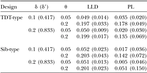
with three children at two LD levels,d¼0.1 (normalized LD,d9¼0.417) andd¼0.2 (d9¼0.833), and two linkage levels,u¼0.05 andu¼0.2, respectively. Only the results on the MLE and MSE of the recombination fraction are shown in Table 2, since the MLEs of the other param-eters, such as allele frequencies and LD coefficient (for LLD), have an excellent accuracy and the statistical power is very high. Table 2 shows that PL yields a large bias (ˆuu) in both TDT-type and sib-type designs. For example, the bias and the root MSE of the estimated recombination fraction are 0.065 and 0.069 for TDT-type design and 0.149 and 0.150 for sib-TDT-type design, respectively, when true parameters areu¼0.2 andd¼ 0.2. This implies that the result from linkage-only analysis is less reliable when association is present. As expected, however, LLD has highly precise estimation. All the absolute values of the bias from LLD are,5% of the parameter values, a conventional criterion for un-biased estimation, and all the MSEs are much less than their counterparts from PL. The bias and the root MSE are0.001 and 0.017 for the TDT-type design and 0.001 and 0.023 for the sib-type design, respectively, whenu¼ 0.2 andd¼0.2.
To demonstrate that LLD can give an unbiased esti-mate of the recombination fraction and further test an arbitrary null hypothesis, say H0:u¼0.1, in such a way
that it has an advantage over FBATs in being capable of identifying tight linkage, we carried out simulations on the basis of a classic TDT-type design consisting of 500 nuclear families with a single child per family under a fully penetrant codominant model. As before, we considered two LD levels,d¼0.1 (d9¼0.417) andd¼ 0.2 (d9¼0.833), and two tight linkage levels,u¼0 and
u ¼ 0.05, respectively. Powers were calculated for the hypotheses H0:u¼0.5 and H0:u $0.1, respectively, in
LLD analysis. The MLE and MSE of the recombination fraction and the corresponding powers are presented in Table 3. As shown in Table 3, LLD gives an accurate estimate and high power for both null hypotheses at
d9¼0.833;e.g., the bias and the root MSE are 0.007 and
0.014, the powers for both H0:u¼0.5 and H0:u $0.1
are 1.0, in the case of u¼0, and the bias and the root MSE are 0.004 and 0.024, and the powers are 0.995 and 0.645, in the case ofu¼0.05, respectively. LLD has reasonable estimation accuracy and test power atd9¼ 0.417. These results suggest that LLD can offer the pos-sibility of distinguishing strong association and loose linkage from weak association and tight linkage, even in the case of only one child per family.
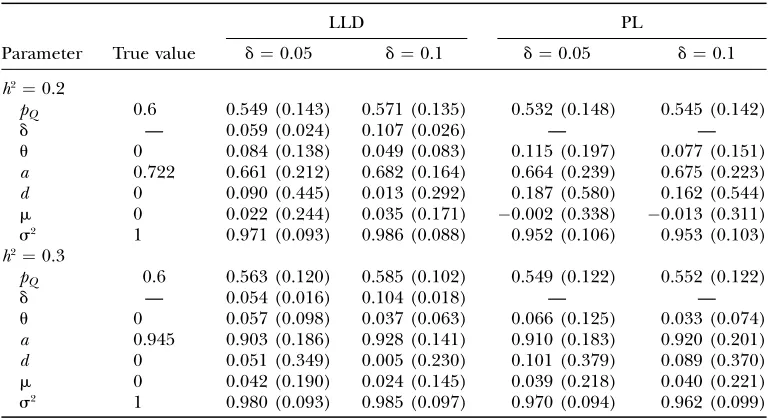
Next we consider a more common case where the dis-ease gene affects a quantitative phenotype. TDT-type data were generated on a sample that consists of 300 families with two children each and 200 families with three children each under an additive model (no dominance effect,i.e.,mQQ¼m1a,mQq¼m, andmqq¼ma, wherem
andaare the mean and additive effect, respectively). We assumed that a marker locus is completely linked to the disease susceptibility locus but with varying degrees of LD (from 0 to 0.1) and heritability (from 0.1 to 0.4). The results of the power comparison of the three methods are summarized in Figures 1 and 2, while only the estimated parameters from LLD and PL are shown in Table 4, be-cause the nonparametric FBAT approach cannot per-form parameter estimation. Figure 1 shows power plotted against LD, where a, b, c, and d are for heritabilities 0.1, 0.2, 0.3 and 0.4, respectively. Figure 2 shows power plotted against heritability, where a, b, c, d, and e are for no LD (d¼0),d¼0.025 (d9¼0.104),d¼0.05 (d9¼0.208),d¼ 0.075 (d9¼0.313), andd¼0.1 (d9¼0.418), respectively. Clearly, the power profiles shown in Figures 1 and 2 support our expectation. As the degree of LD increases, so does the power of the FBAT and LLD, whereas that of PL is almost unchanged or increases little (Figure 1, a– d). The power also increases with heritability for most cases, but when there is no LD, the FBAT has no power regardless of the value of the heritability (Figure 2a). Generally speaking, it appears that LLD is the most powerful, followed by PL and then the FBAT when LD is absent or weak (d9 ,0.2; Figure 2, a and b) or by the FBAT and then PL when LD is strong (Figure 2, c–e). Other than the cases of no LD, where PL has power close to that of LLD, LLD is much more powerful than PL. Also, LLD always performs better than the FBAT, even under situations with strong LD (d9$0.313), where the TABLE 2
Average MLEs (and root MSEs) of the recombination fraction (u) from pure linkage analysis (PL) and combined linkage
and association analysis (LLD) at two levels of LD for TDT-type and sib-type designs, respectively
Design d(d9) u LLD PL
TDT-type 0.1 (0.417) 0.05 0.049 (0.014) 0.035 (0.020) 0.2 0.197 (0.033) 0.178 (0.049) 0.2 (0.833) 0.05 0.050 (0.009) 0.020 (0.030) 0.2 0.199 (0.017) 0.135 (0.069)
Sib-type 0.1 (0.417) 0.05 0.052 (0.023) 0.017 (0.036) 0.2 0.203 (0.043) 0.142 (0.072) 0.2 (0.833) 0.05 0.051 (0.013) 0.005 (0.046) 0.2 0.201 (0.023) 0.051 (0.150)
TABLE 3
Average MLEs (and root MSEs) of the recombination fraction (u) and powers for two null hypotheses (H0:u¼0.5 and H0:
u$0.1) from combined linkage and association analysis (LLD) at two levels of LD for the TDT design
d(d9) u LLD H0:u¼0.5 H0:u $0.1
power of the FBAT approaches that of LLD. This is not surprising, because more than one sibling is available in our simulations and hence, in theory, information on allele sharing between siblings should contribute to de-tecting linkage except for the case of no linkage, where there is no practical importance as there is no interest in testing for linkage with a type I error. The power com-parison indicates that the union of two complementary components of information allows LLD to be more powerful.
Unlike FBATs, our new approach can also achieve parameter estimation for gene effects, allele
frequen-cies, LD coefficient, and recombination fractions, so that it can provide more knowledge regarding disease etiology. Table 4 lists some typical results on the com-parison between LLD and PL, but the results are not shown when LD is absent or weak, as LLD has an esti-mated result similar to that of PL. In the latter situation, both LLD and PL gave unbiased estimates, although LLD appeared to have slightly larger MSE, but the dif-ference was very small. Such results are highly consistent with our expectation because the assumption of linkage equilibrium is indeed satisfied for linkage-only anal-ysis while one needs to estimate one more unknown
Figure1.—Power of FBAT, PL, and LLD plotted against LD coeffi-cientd(d9) at the 0.05 significance level for four heritabilities: (a)h2¼ 0.1, (b)h2¼0.2, (c)h2¼0.3, and (d)h2¼0.4, respectively.
parameter for LLD. But for cases with slightly stronger LDs, such as d9 $ 0.208, LLD gained much improve-ment in estimation accuracy, which is reflected by bias and MSE, over linkage-only analysis (see Table 4). The bias and MSE of the estimated parameters from LLD are almost uniformly less than their counterparts from PL. This is in good agreement with theoretical expectations. In general, the estimation accuracy increases with LD, and LLD improves more than PL. The magnitude of improvement differs with the various parameter values. The estimates of recombination fraction and genetic effects are greatly affected by LD level, while those of population mean and variance are less affected. In some cases, ignoring LD may result in a large bias and MSE in PL. The comparison of parameter estimation strongly indicates that it is necessary to capitalize on the infor-mation from population association to get a better and more reliable estimation.
APPLICATION
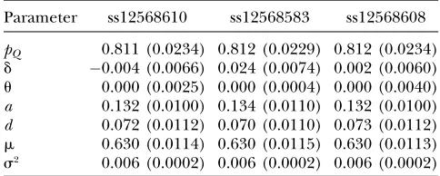
To demonstrate its use, we applied our new algorithm to a BMD genetic study conducted at Creighton Univer-sity. A total of 1873 subjects from 405 Caucasian pedi-grees containing 740 parents/grandparents and 434 sibships were included in the study. The pedigrees varied in size from 3 to 12 and the mean size was 4.86 while the sibships ranged from 1 to 10 and averaged 2.61. Three SNPs within the vitamin D (1,25-dihydroxyvitamin D3) receptor (VDR) gene, ss12568610, ss12568583, and ss12568608, were chosen to test association with BMD. A detailed description of the clinical subjects and SNP-related information, such as primers/probes and
geno-typing conditions, has been reported in a separate study (Liuet al.2005). Several BMD-related traits were mea-sured in the study (Liuet al.2005) and we used the BMD at the one-third region of the wrist as an example here. The phenotypic values of the BMD range from 0.349 to 0.997. Our segregation analysis suggested that there is a major gene underlying this trait (data not shown). The coefficients of skewness and kurtosis of the residual ef-fects are 0.123 and 3.175, respectively, which can be re-garded as having an approximately normal distribution. The results analyzed by FBAT and our LLD approach are presented in Tables 5 and 6 forP-values, MLEs, and standard errors (SEs), respectively. The threeP-values in Table 5 are for null hypothesesu¼0.5,u $0.2, andu $
0.1, respectively, in LLD analysis, while theP-values are foru¼0.5 in FBAT. After correction for multiple testing, the LR statistic still remains highly significant (mini-mumP¼0.001 for H0:u¼0.5), whereas the FBAT
sta-tistic shows only marginal significance (P ¼0.040) for ss12568583. Furthermore, the results of parameter estimation show that all the three SNPs are very tightly linked to the putative disease gene,i.e., have near zero estimated recombination fractions and small SEs, but different frequencies from those of this gene (see Table 6). All estimates from the three SNPs are very consistent, which indicates that, very likely, a gene responsible for BMD is located within or near the VDR gene but the genotyped SNPs do not seem to be the causal variant. The MLEs of d9 are 0.045, 0.177, and 0.021 for SNPs ss12568610, ss12568583, and ss12568608, respectively, suggesting that the associations between the gene and the SNPs are weak. This may be the reason why this gene can elude most FBAT gene-hunting strategies such as QTDT and FBAT. Our approach also gave estimates of TABLE 4
Average MLEs (and root MSEs) from the approach of either pure linkage (PL) or combined linkage and association analysis (LLD)
Parameter True value
LLD PL
d¼0.05 d¼0.1 d¼0.05 d¼0.1
h2¼0.2
pQ 0.6 0.549 (0.143) 0.571 (0.135) 0.532 (0.148) 0.545 (0.142)
d — 0.059 (0.024) 0.107 (0.026) — —
u 0 0.084 (0.138) 0.049 (0.083) 0.115 (0.197) 0.077 (0.151)
a 0.722 0.661 (0.212) 0.682 (0.164) 0.664 (0.239) 0.675 (0.223)
d 0 0.090 (0.445) 0.013 (0.292) 0.187 (0.580) 0.162 (0.544)
m 0 0.022 (0.244) 0.035 (0.171) 0.002 (0.338) 0.013 (0.311)
s2 1 0.971 (0.093) 0.986 (0.088) 0.952 (0.106) 0.953 (0.103)
h2¼0.3
pQ 0.6 0.563 (0.120) 0.585 (0.102) 0.549 (0.122) 0.552 (0.122)
d — 0.054 (0.016) 0.104 (0.018) — —
u 0 0.057 (0.098) 0.037 (0.063) 0.066 (0.125) 0.033 (0.074)
a 0.945 0.903 (0.186) 0.928 (0.141) 0.910 (0.183) 0.920 (0.201)
d 0 0.051 (0.349) 0.005 (0.230) 0.101 (0.379) 0.089 (0.370)
m 0 0.042 (0.190) 0.024 (0.145) 0.039 (0.218) 0.040 (0.221)
the penetrance parameters. As shown in Table 6, the gene has a large genetic effect and displays an incom-pletely dominant mode of inheritance. In summary, our results indicate that the VDR gene is significantly linked to that for BMD, especially for SNP ss12568583.
DISCUSSION
This study was motivated by the fact that traditional mapping methods, e.g., FBATs and the allele-sharing method, utilize only one component of genetic in-formation, either on linkage or on association, often leading to inefficiency and inaccuracy, although they have desirable properties in some specific cases,e.g., if the assumption of no LD is approximately satisfied in linkage analysis or if the marker tested is exactly the trait gene itself in FBATs. Owing to its ignoring association, the weakness of linkage analysis motivated Rischand Merikangas(1996) to conclude that the allele-sharing method may be hardly up to the task of identifying genes underlying complex traits. On the other hand, however, the TDT may be not as ideal as Risch and Merikangas (1996) claimed because such a perfect case (i.e., perfectly associated, with no recombination and the same allele frequencies) rarely occurs in real data sets, even in a fine-mapping context. Mostly, there are less extreme cases with diverse degrees of LD be-tween both tightly linked loci and loosely linked loci,
arising from mutation, recombination erosion, or pop-ulation admixture. Therefore, it is necessary to develop new approaches that can improve the FBAT’s power for successful gene hunting. Heuristically, exploiting in-formation on allele sharing contained in each sibship can achieve this aim and also circumvent the weakness that association is required for linkage to be detected. Such attempts have been pursued by a number of re-searchers (e.g., Zhao et al.1998; Xiongand Jin 2000; Cantoret al. 2005; Liet al.2005). In our previous study (Lou et al. 2005), we reported the development of a statistical framework with two hierarchies. In this article, we address a further issue, i.e., developing mapping models with an arbitrary number of hierarchies to han-dle complex pedigrees. Thus, the proposed approach not only is capable of accommodating multiple loci and/or multiple alleles so that it is easy to tackle interval mapping, multiple interval mapping, and epistasis mod-els, but also allows for diverse types of traits and pedigree structures. Haplotypes in founders contribute infor-mation for an association study while informative and partially informative meioses do so for linkage analysis. We unify segregation, linkage, and association analyses into a comprehensive mapping strategy and thus can capture the two complementary aspects of the genetic architecture. The proposed approach has the proper-ties of both linkage analysis and association analysis. From the viewpoint of linkage, it is a LOD score method that is adaptive to the amount of LD. It can make use of LD, if it is indeed present, while it reduces to the standard LOD method when LD is weak or absent. From another viewpoint, it is an association study that incor-porates haplotyping analysis in pedigrees and genotyp-ing by a progeny test at a disease locus. For sgenotyp-ingleton data, it reduces to a parametric association study (e.g., Louet al. 2003; Shibataet al. 2004). Although the EM algorithm rather than the quasi-Newton method is used to maximize the likelihood function, our approach is a direct generalization of that of Cantoret al. (2005) to multiple loci. The model of Li et al. (2005) is also a specific application of the new method, which assumes that the candidate SNP is completely linked to the disease locus and that flanking markers are in linkage equilibrium with one another, the SNP, and the disease TABLE 5
A comparison ofP-values for association of VDR SNPs with BMD
SNP Physical position Domain Allelea Allele frequencyb
FBAT LLDP-value
P-value u¼0.5 u $0.2 u $0.1
ss12568610 45,470,003 Intron 8 G/A 0.419 0.108 0.082 0.123 0.199
ss12568583 45,507,963 59-UTR G/A 0.280 0.040 0.001 0.021 0.081
ss12568608 45,468,924 Exon 9 T/C 0.408 0.246 0.102 0.158 0.241
a
The boldface type in SNP polymorphisms represents minor alleles.
b
The allele frequencies are for minor alleles.
TABLE 6
MLEs (and standard errors) for allele frequency, LD, recombination fraction, additive and dominance
effects, mean, and variance on using different VDR SNPs
Parameter ss12568610 ss12568583 ss12568608
pQ 0.811 (0.0234) 0.812 (0.0229) 0.812 (0.0234)
d 0.004 (0.0066) 0.024 (0.0074) 0.002 (0.0060)
u 0.000 (0.0025) 0.000 (0.0004) 0.000 (0.0040) a 0.132 (0.0100) 0.134 (0.0110) 0.132 (0.0100) d 0.072 (0.0112) 0.070 (0.0110) 0.073 (0.0112)
m 0.630 (0.0114) 0.630 (0.0115) 0.630 (0.0113)
locus. Both the corresponding LR statistics, testing for linkage equilibrium and complete LD, can be constructed by using the new approach.
Another contribution of this article is that it shows, through systematic simulation studies and an application, the important conclusion that a mapping bonus can be obtained by combined linkage and association analysis without any increase in experimental expense. This is highly consistent with theoretical expectation. First, the improvement in mapping resolution arises from the marriage of linkage and association. In a gene-hunting context, latent data exist such as disease genotype, in-heritance vector, and linkage phase. Parameter estimation and statistical inference rely on accurate genetic recon-struction of such ambiguous data,i.e., statistical imputa-tion. Violation of the assumption of linkage equilibrium leads to inaccurate imputation in pure linkage analysis so that it may give a biased result, as demonstrated in this article. On the other hand, the assumption of linkage equilibrium also affects imputation precision, owing to its resulting in a likelihood that retains maximum uncer-tainty about which component of the mixture distribution generates the data, and hence is least informative for the recombination parameter u. Theoretically, integrating both complementary components increases imputation accuracy, leading to improvement in mapping accuracy, precision, and power over traditional linkage analysis. Intuitively, linkage induces more gene concordance be-tween related individuals having similar phenotypes, while the opposite holds true for those with disparate phenotypes. Incorporating this information, which FBATs fail to do, gives our LLD approach a higher power than that of FBATs. This type of phenomenon has also been widely observed with comparisons of the TDT, the conventional affected sib pairs, and combined methods (Huangand Jiang1999; Wicksand Wilson 2000; Lazzeroni2002). Both our simulation and real data studies support our theoretical expectation.
Second, the improvement may also come from two other potential sources, although they are not explored in this article. The LLD approach integrates population-based association analysis and pedigree-population-based linkage analysis into a coherent framework so that it can handle diverse types of data, including full sibs, half sibs, cous-ins, nuclear families, extended nuclear families, com-plex pedigrees, and singletons, as well as their mixtures. Unlike those of Huangand Jiang(1999), Wicksand Wilson(2000), and Lazzeroni(2002), which require only affected pairs with at least one heterozygous par-ent, our approach allows for analyzing any type of data structure, including singletons and pedigrees without any informative meioses, which do not contribute infor-mation to linkage parameter(s) but do inform associa-tion parameter(s). Without dropping any type of mapping data, we make use of data to the maximum extent, lead-ing to the possibility of improvlead-ing mapplead-ing perfor-mance. Furthermore, our flexible framework is easily
applied to a multipoint analysis. It has been well doc-umented that multipoint analyses can extract more statistical information than pairwise ones and thus may substantially increase the power and reduce spurious results (Lathropet al.1984, 1985). Conceivably, unify-ing multilocus linkage and association mappunify-ing will further improve mapping resolution.
Our current version of the program is capable of handling five to six loci on a PC computer if only limited amounts of data are missing. Although it allows for more loci and alleles on a workstation or a PC cluster with more memory and storage, computation can be very time-consuming for a large number of loci and alleles because the required memory and time exponentially increase with the number of loci. To avoid a formidable computational burden, the simulation-based versions of the EM algorithm such as stochastic EM and Markov chain Monte Carlo (MCMC) EM (Thompson 1994; Celeuxet al.1996), based onestimatingconditional pos-terior probabilities in the E-step rather than computing them exactly, can be used. The approximate methods based a composite likelihood (e.g., Rannalaand Slatkin 2000) also seem to be the feasible ways to tackle this problem. The relevant study is under way.
Moreover, unlike the model-free approaches such as allele sharing and FBATs, which can tell us only whether linkage or association exists but fail to provide any esti-mates of what values they have, the proposed LLD ap-proach can simultaneously provide parameter estimation of genetic distance, allelic association, and genotype– phenotype relationship and also perform various types of hypothesis testing. For example, we can perform a com-parison of the analyses, including or not the LD infor-mation to assess the validity of the LD model assumptions. Thus, this approach exposes more genetic mechanisms than FBATs to genetic etiology and hence increases the predictability of gene mapping.
Finally, as pointed out by Pe´ rez-Enciso(2003), given the diversity of genetic architectures and population histories, it is unlikely that a single statistical approach will be valid for all cases. The approach described here is subject to the same limitations faced by all model-based methods,i.e., the requirement of a correct, or close to correct, model for the trait under study. If the model for predicting disease status from phenotypes is not suffi-ciently well known, this approach cannot perform well. Therefore, this model-based LLD approach should serve as a supplement to model-free methods in track-ing the gene(s) underlytrack-ing complex diseases, once model-free methods have suggested how many loci are involved and their approximate locations in the genome (Elston 1998).