ABSTRACT
GIFFEN, NICHOLAS J. Particle Size Segregation In Granular Avalanches: A Study In Shocks. (Under the direction of Michael Shearer.)
In this thesis, we explore properties of shock wave solutions of the Gray-Thornton model for particle size segregation in granular avalanches. In these avalanches, particles segregate by size when subject to shear. As the particles roll across each other, other particles fall into the gaps that form, with smaller particles more likely to fit. These small particles fall to the bottom of the avalanche and force the larger particles upward. These processes are calledkinetic sieving and squeeze expulsion. The Gray-Thornton model is a nonlinear scalar conservation law expressing conservation of mass under shear for the concentration of small particles in a bidisperse mixture. In this model, the velocity (and thus, shear) is a function of the height of the avalanche. We first discuss characteristic surfaces of the model, which are used in combination with shock waves to construct and analyze solutions of the model.
Shock waves are weak solutions of the partial differential equation across which the con-centration of small particles jumps. For a linear velocity profile, we give criteria on smooth initial conditions under which a shock wave forms in the interior of the avalanche in finite time. Additionally, numerical simulations show how and when these shocks form, verifying our analysis.
Linear velocity profiles are not always present in granular materials, especially in the case of boundary driven shear. Thus, we analyze shock formation from smooth initial data under a general increasing velocity profile. Additionally, we analyze the short time solution of the mixing zone under an increasing velocity profile. Here, we present several cases, with each case more general than the previous one. For each case, we analyze the structure of the mixing zone as much as possible, and discuss limitations to the more general cases. Numerical simulations show how the mixing region evolves for each case.
Particle Size Segregation In Granular Avalanches: A Study In Shocks
by
Nicholas J. Giffen
A dissertation submitted to the Graduate Faculty of North Carolina State University
in partial fulfillment of the requirements for the Degree of
Doctor of Philosophy
Applied Mathematics
Raleigh, North Carolina
2010
APPROVED BY:
Ralph Smith Pierre Gremaud
Alina Chertock Michael Shearer
BIOGRAPHY
Nicholas J. Giffen (Nick) was born October 28, 1983 in Charlottesville, Virginia. He grew up as part of a large, active family, consisting of mom, dad, one sister and five brothers. Never a dull moment to be had in the family, he grew up playing a variety sports in his backyard with his siblings. Throughout high school, Nick played the trombone, and he would eventually take his talents to James Madison University where he began as a music major.
At college, Nick switched majors after his second year, and chose mathematics instead. Upon switching majors, Nick met with Dr. James Sochacki, a professor in the mathematics department, to plan out how he would meet all the requirements for a math major in his final two years of college. Dr. Sochacki would become Nick’s advisor, and gave him his first taste of research, a summer project on the chaotic double pendulum. Having felt like he experienced only two years of college, Nick decided to apply to graduate school, and was accepted at N.C. State.
For nearly the first two years, Nick was set on only obtaining his masters, but after taking one semester of partial differential equations with Dr. Michael Shearer, Nick found his calling in the subject, and decided to stay on as a Ph.D. student as an RA under Dr. Shearer.
ACKNOWLEDGEMENTS
I would like to thank:
• My advisor Michael Shearer for his patience, encouragement, and wisdom. I have learned
a lot from you about math and life, and will apply it in my future experiences.
• My committee members Ralph Smith, Alina Chertock, Pierre Gremaud and Peter
Bloom-field for their insightful comments and questions and for all they have taught me.
• All of my friends, in and out of the math department, with whom I have enjoyed many
good times.
• The professors at N.C. State that have taught me so much.
• The members of AMGSS and the Daniels Lab group for critiquing my work and
presen-tations, and sharing their knowledge with me.
• The National Science Foundation for providing the funding for this research under grants
DMS-0604047 and DMS-0636590.
• The staff members who keep the mathematics department organized and running smoothly.
• The professors at James Madison University in music and math, for providing me with a
solid academic foundation, especially Dr. Sochacki.
• The members of my soccer teams for some quality teamwork and fun on the field.
• My family for their love and support. Thanks for always being there when I need you
TABLE OF CONTENTS
List of Figures . . . vi
Chapter 1 Introduction to Segregation in Granular Materials . . . 1
1.1 Overview of Granular Materials . . . 2
1.1.1 Properties of Granular Materials . . . 2
1.1.2 Importance of Granular Materials . . . 3
1.1.3 History of the Study of Granular Materials . . . 3
1.2 Segregation in Granular Materials . . . 5
1.2.1 Introduction to Granular Segregation . . . 5
1.2.2 Kinetic Sieving . . . 6
1.2.3 Granular Segregation Models . . . 6
1.3 Summary of Thesis Chapters . . . 7
Chapter 2 The Gray-Thornton Model . . . 9
2.1 Derivation and Formulation . . . 9
2.2 Modifications of the Gray-Thornton Model . . . 13
2.2.1 Linear Velocity Profile . . . 14
2.2.2 Nonlinear Velocity Profile . . . 15
2.2.3 Uniformity Downslope . . . 16
2.3 Numerical Simulations of (2.18) . . . 17
Chapter 3 Characteristics and Shocks . . . 19
3.1 Characteristics . . . 19
3.2 Shocks . . . 21
3.3 Shock Stability . . . 22
Chapter 4 Shock Formation . . . 24
4.1 Analysis of interior shock formation . . . 25
4.2 Shock formation example . . . 29
4.3 Shock formation simulations . . . 31
Chapter 5 Shock Breaking . . . 39
5.1 The Mixing Zone . . . 42
5.2 A Special Mixing Zone . . . 55
Chapter 6 Scaling the Gray-Thornton Model . . . 59
Chapter 7 Modifications to the Gray-Thornton Model . . . 62
7.1 Shock Formation . . . 65
7.2 Generalized Shock Wave Breaking . . . 70
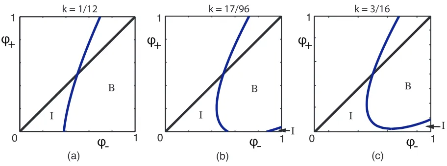
7.2.2 Depth-Dependent Segregation Rate, ϕ−= 1, ϕ+= 0 . . . 74
7.3 Depth-Dependent Segregation Rate,ϕ−> ϕ+ . . . 76
7.3.1 Interior Solution . . . 79
7.3.2 Boundary Shocks . . . 80
7.3.3 Examples . . . 81
7.3.4 1D Shock Formation . . . 86
Chapter 8 Conclusions . . . 88
8.1 Future Directions . . . 90
LIST OF FIGURES
Figure 4.1 Phase portrait for system (4.3). . . 27
Figure 4.2 Shock formation withv0, w0 >0. . . 34
Figure 4.3 Shock formation withv0 >0, w0 <0. . . 35
Figure 4.4 Shock formation withv0, w0 <0. . . 36
Figure 4.5 No shock formation withv0 <0, w0<>0. . . 37
Figure 4.6 Case (A): shock formation from∇ϕ0(r) = 1−r. . . 37
Figure 4.7 Case (B): shock formation from∇ϕ0(r) =r. . . 38
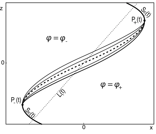
Figure 5.1 Schematic of the mixing zone joining constant values ϕ− > ϕ+.. . . 43
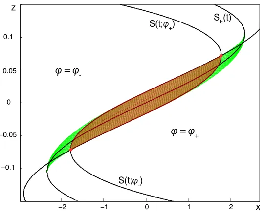
Figure 5.2 The mixing zone and the region bounded by S(t;ϕ−) and S(t;ϕ+). . . . 46
Figure 5.3 Cubic Case: classifying breakdown of M1(t). . . 50
Figure 5.4 Cubic case: (a) The solution forM2(t). (b) Zoomed in aroundP+(t). . . 51
Figure 5.5 Cubic case: The solution M3(t). . . 53
Figure 5.6 Quadratic Case: k= 14, m= 1, S = 1, ϕ+ = 0, ϕ−= 1, t= 0.1 . . . 57
Figure 6.1 Scaled solutions fort= N 10 forN = 1, . . . ,10. . . 61
Figure 7.1 (ϕ, z) phase portrait for (7.3) . . . 64
Figure 7.2 (a) PDE simulation for Ma(0.65) (b) Numerical solution to (7.31) for Ma(0.65) . . . 73
Figure 7.3 PDE simulation for the evolution of Ma(t) withϕ+= 0.1. . . 73
Figure 7.4 (a) PDE simulation for Mb(0.65) (b) Numerical solution to (7.38) for Mb(0.65) . . . 76
Figure 7.5 Mc(t) at t= 0.65 withϕ−= 1 . . . 78
Figure 7.6 Mc(t) at t= 0.65 withϕ−= 0.9 . . . 79
Figure 7.7 Contour plots of the evolution of ϕ(z(t), t) from equation (7.42) with S(z) = 1 and initial condition ϕ(z(0),0) =ϕ0(z0) = 12. . . 82
Figure 7.8 Solution of (7.44) and (7.49) with boundary shocks given by (7.51-7.52) for the case where S(z) = 1, ϕ0(z0) = 1 2. . . 83
Figure 7.9 Contour plots of the evolution of ϕ(z(t), t) from equation (7.42) with S(z) = e−z and initial condition ϕ(z(0),0) = ϕ0(z0) = 1 2. The contour lines are at intervals of 0.005. . . 84
Chapter 1
Introduction to Segregation in
Granular Materials
Many of us start our day by pouring ourselves a bowl of cereal for breakfast. Later in the day, we might drive past a sign that reads ”fallen rock zone”. In the evening, many people take medications in the form of a pill to fight off the accumulation of aches or pains throughout the day. What most of us don’t realize, is that each of these common daily events involve a complex area of science called granular materials. The study of granular materials and the theory of their dynamics has become an increasingly important area of study among scientists, engineers, and mathematicians. Developments in the theory of granular materials have helped with advancements in many aspects of our daily lives, from morning to night, from home to work to vacation.
1.1
Overview of Granular Materials
Granular materials are defined as a collection of discrete solid macroscopic particles that are large enough so that they are not subject to thermal motion fluctuations [2]. Therefore, tem-perature changes do not affect granular materials on the macroscopic level [32]. Interactions between individual grains are energy dissipative; for example, inelastic collisions display this behavior. Some granular materials occur naturally, such as nuts, sand, soil, and rice. Other granular materials are manufactured, such as ball bearings, pharmaceuticals, and beads. A dry granular material is one that is either absent of interstitial fluid, such as air or water, or is modeled as such. A granular material is called noncohesive if there are no attractive forces between particles. Thus, the shape of the system is determined by either external boundaries or gravity.
1.1.1 Properties of Granular Materials
Granular materials can display properties of all three phases of matter: solids (a pile of rocks), liquids (sand flowing through a funnel), and gases (strongly agitated materials). However, granular materials also display properties that are different from those of the three states of matter [36]. For example, a granular material in a static pile will begin to flow like a liquid when tilted beyond a critical angle. As this happens, the liquid-like flow occurs only in the boundary layer. This is different from the behavior of ordinary liquids, where the entire fluid flows. However, flowing granular material can then jam into a solid-like state, such as flow out of a poorly designed hopper. The difference between gaseous-like granular materials and a dense gas is that the collisions in granular materials are inelastic. A dense gas exhibits elastic collisions. Due to the dissipative interactions between individual particles in a granular material, the material will come to rest unless energy is continuously supplied to the system. While solid, liquid, and gas dynamics are described by well-developed theories, much less is understood about the variety of properties displayed by granular materials.
dominates interparticle forces, such as electrostatic, air drag, van de Waals, and capillary forces. Thus, particle sizes must be larger that 500µm [15]. All granular mixtures are dry, noncohesive,
and dense, meaning particle interactions occur frequently and simultaneously with multiple neighbors. Contacts in the material are non-collisional, resulting in little to no momentum transfer between particles. Finally, a bidisperse mixture consists only of two types of particles that display a difference in only one physical property, such as size, density, shape or roughness.
1.1.2 Importance of Granular Materials
The flow of granular materials is of importance in many areas of science and industry. Geo-physical events such as debris flows [9, 28, 29, 30],[47], rockslides[3, 10], lahars [69], pyroclasitc flows [6, 31], and snow and ice avalanches [35] are all large-scale flows that involve particulate solids in a fluid-like state. The nature of these events may pose a great threat to human life and can cause considerable property damage [25, 26, 27, 52, 61, 62] underscoring the importance of studying such granular flows. Problems that arise in modeling these events include predicting runout distance, velocities, and flow over a complex topography in order to define a safety zone to minimize loss of life and property damage. The fluid-like behavior of these systems in combination with the steep slopes that they occur on have yielded numerous models, physical and scaling laws, and experimental results about the flow of granular materials down an incline. In addition to the geophysical importance for studying granular materials, the study of their flow also arises in engineering applications involving transport of minerals, pharmaceuticals, and certain foods (such as beans and cereals). The mining and bulk chemical industries also process large amounts of granular materials. In fact, the pharmaceutical, food, and bulk chemical industries produce an estimated one trillion killograms of granular materials per year [60].
1.1.3 History of the Study of Granular Materials
seeds. One of the first applications of granular flow was the hourglass, which was in common use by the thirteenth century [54]. In the late eighteenth century, C. de Coloumb (1736-1806) wrote a paper in which he proposed the idea of static friction [32]. In his paper, he draws conclusions about the equilibrium of earthen embankments and stability of stone structures, leading to his laws of dry friction between solids. His work would later be extended to granular materials when in 1857 W. Rankine considered theoretical implications of friction in granular materials. Rankine developed the principles of active and passive states of particles [51].
From the beginning of the twentieth century on, granular materials have become an in-creasingly important field of study. Early hypotheses [16, 18, 37] to explain fluidization often lacked a detailed computation of the flow development, and direct observation of the dynamics of granular avalanches had been difficult to make. The difficulty in describing these granular flows arises from an uncertainty in the constitutive equations. The dense regime cannot rely on a kinetic approach to resolve the constitutive equations due to the multicontact interactions between particles as well as friction.
Hutter.
1.2
Segregation in Granular Materials
The flow of granular materials also leads to an interesting phenomenon in that dissimilar par-ticles mix and segregate. The blending and separating of dissimilar parpar-ticles is of significant importance in the industries mentioned in§1.1.2. In some cases, such as the mineral processing
industry [70] and the pharmaceutical industry segregation is desired. On the other hand, in processes where the goal is to mix two cohesionless materials [20, 45, 59] segregation is to be avoided to achieve the desired mixture. Incorrect blending or separation of dissimilar particles often reduces the product quality, and in some cases, can even lead to safety concerns. For example, incorrect blends can create dosage variations in pharmaceuticals, flavor variations in foods, and even gas flow problems in chemical reactors [65]. An inconsistency in a blend can often lead to the rejection of an expensive batch, causing the manufacturers a significant loss of money and reputation. The importance of mixing and segregation highlights the need to have an effective model that describes these processes in regards to dissimilar particles.
1.2.1 Introduction to Granular Segregation
1.2.2 Kinetic Sieving
Consider a system with particles of two different sizes. Experiments and simulations have shown that under shear, vertical segregation with large particles on top of small particles occurs through a process known as kinetic sieving. This process occurs in slow, dense, dry granular flows, which drives particle size segregation based on the combination of percolation (void filling) and squeeze expulsion. This mechanism is often observed when cohesionless mixtures of different sized particles flow down a rough incline. Here, velocity-induced shear is the physical force that drives the mechanism of kinetic sieving. Void filling occurs when the particles roll and tumble over each other, creating fluctuations in the local void ratio. As gaps form in between particles the small particles tend to fall down in between and fill the gaps. The larger particles are pushed upward by squeeze expulsion, which occurs due to an imbalance in contact forces on a particle which squeezes it up or down. Combining the two, the net percolation velocity of both large and small particles is obtained. This mechanism was identified and quantified in the classic paper of Savage and Lun [56].
1.2.3 Granular Segregation Models
mechanics to introduce the idea of kinetic sieving. They provide a comparison between their theory and their experimental results as well as the experimental results from Bridgewater and colleagues [5].
While the Savage and Lun model has the desired feature of predicting steady-state particle size distribution in a steady uniform flow, one of the drawbacks of their model is that it predicts segregation by kinetic sieving even when gravity is not present. This is a shortcoming in the model, since the percolation of small particles downward by void filling is a gravity driven process. While segregation may occur when there is no gravity, it is driven instead by spatial gradients in the fluctuation energy of dissimilar particles [33, 71]. In 2005, Gray and Thornton introduced a model that was closely linked to Savage and Lun’s, but provided a means to introduce gravity into the model [23]. This model is the focus of the work in this thesis.
1.3
Summary of Thesis Chapters
This thesis considers concentration shocks of particle size in granular materials. The formation and stability of these shocks along with the subsequent evolution of unstable concentration shocks are the main topics touched on in this work. Specific analysis, simulations, and numerical solutions are all tied together throughout the thesis to confirm all results.
The model developed by Gray and Thornton [23] is considered for particle-size segregation in granular materials. Chapter 2 deals with the introduction, derivation, and formulation of the model. Modifications are developed to fit the model to generalize the problems of shock formation and shock breaking. A discussion of the numerical method employed in our MATLAB code for the model concludes the chapter.
multidimensional conservation laws by Conway [7] and Majda [40]. The main difference in the use here, is due to shear within the flow which gives rise to the non-constant coefficients in the PDE. A full analysis of the two-dimensional version of the Gray-Thornton model completely characterizes shock formation from smooth initial data. Numerical simulations and subsequent analysis are used in combination to further verify the analysis. The first part of Chapter 5 deals with the problem of shock wave breaking after a concentration shock loses stability in the case of two dimensional flow under constant shear. The resulting mixing zone has a structure that evolves in three stages. In the first stage, we construct the solution exactly, while the second and third stage constructions consist of shocks and rarefactions that are pieced together to form the mixing region. The latter two stages are constructed through explicit evolution of the first stage, and numerically in the unknown parts of the region. The second part of Chapter 5 concerns a special case of the mixing zone problem, where a piecewise quadratic concentration shock breaks. Chapter 6 talks about a scaling for the Gray-Thornton model, specifically applied to the piecewise quadratic case from Chapter 5.
Chapter 2
The Gray-Thornton Model
Gray and Thornton [23] formulated a PDE conservation law as a model for particle-size segre-gation using binary mixture theory [46, 67], which allows for every point in the material to be occupied by large and small particles. As a result, velocities, pressures, and densities of both phases can be defined everywhere in the material. Individual constituent momentum balances are used to encapsulate the effects of gravity and the resulting modeling is able to compute the temporal and spatial evolution of particle size distribution in a three-dimensional dry granu-lar flow. The main assumptions made by the Gray-Thornton model are that the mixture is bidisperse, all particles have the same bulk density, the bulk flow is incompressible, normal accelerations can be neglected, and diffusive remixing is negligible. In a later paper, Gray and Chuganov include diffusive remixing [21].
2.1
Derivation and Formulation
The variable of interest in the Gray-Thornton model is the concentration of small particles (the ratio of the volume of small particles to the total volume of small and large particles). This variable ϕ is a function of space in three dimensions (x, y, z) and time t. The volume
cross-slope direction. The slope is at an angle ζ to horizontal. The bulk velocities in thex,y,
and z-directions are given by u,v, and w, respectively.
Another assumption is that segregation occurs only in the direction normal to the base of the avalanche z. Therefore, the velocity in the z direction has two components: the bulk
velocity and the segregation velocity. The equations for the normal constituent velocities are simply derived from the conservation of momentum equation for each constituent.
ρνDνu
ν
Dt =−∇p
ν+ρνg+βν, ν=s, l, (2.1)
wheresand lrepresent the small and large particles,u= (u, v, w), andDν/Dt=∂/∂t+uν· ∇
is the material derivative. The partial densities, velocities, and pressures are given byρν,uν,
andpν, respectively. The gravitational acceleration is given byg, and the interaction force (the
force exerted by the other constituent on phaseν) is given by βν. In mixture theory, variables
are either intrinsic or partial. In this case, an intrinsic variable is independent of the volume fraction of small or large particles. On the other hand, a partial variable is related to an intrinsic variable through a linear volume fraction scaling. The velocity field is the only exception, and is identical in both the partial and intrinsic cases. The bulk density and pressures are related to the constituent quantities by
p=ps+pl (2.2)
and
ρ=ρs+ρl (2.3)
In mixture theory, partial variables are related to their physical, or intrinsic, counterparts. In standard mixture theory, the partial and intrinsic velocity fields are identical, while the other fields are related by linear volume fraction scalings
where the superscript * denotes an intrinsic variable and where ϕs = ϕand ϕl = 1−ϕ. The
forces βs and βl are equal in magnitude, opposite in direction, and the intrinsic densities are
equivalent and constant, thus equal to the bulk density.
Under the assumption that the normal acceleration is negligible, the sum of the momentum balance components (2.1) for each constituent implies
∂p
∂z =−ρgcosζ. (2.5)
Since ρ is constant, integrating through the depth of the avalanche h shows the bulk pressure
is hydrostatic:
p=ρg(h−z) cosζ. (2.6)
When the small particles percolate between the large particles, they support less than their share of the overburden pressure, meaning the large particles must carry more of the load. Therefore, a new pressure scaling is introduced
pl=flp, ps=fsp (2.7)
where fl and fs determine the proportion of the hydrostatic load carried by large and small
particles respectively. Equation (2.2) impliesfl+fs = 1.
Experimental observations of the kinetic sieving process suggest an analogy with the per-colation of fluids through porous solids, thus, Darcy’s law motivates an interaction drag of the form [46]
βν =p∇fν−ρνc(uν −u), ν=l, s (2.8)
wherec is the coefficient of inter-particle drag andu= (ρlul+ρsus)/ρ.
The normal constituent velocitieswv are obtained by substituting equations (2.5)-(2.8) into
are negligible, to get
ϕνwν =ϕνw+ (fν−ϕν)(g/c) cosζ, ν =l, s. (2.9)
The significance of fν is now clear, for if fν > ϕν then particles rise and if fν < ϕν then
particles fall. When the two quantities are equal, there will be no motion of particles relative to the bulk. Therefore, the funcionfν must satisty the constraint that if only a single type of
particle is present, it must support the entire load, i.e.
fl= 1, when ϕs= 0, fs= 1, when ϕs= 1.
(2.10)
The simplest nontrivial functions that satisfy (2.10) and fl+fs = 1 are fl =ϕl+Bϕsϕl and
fs=ϕs−Bϕsϕl. Substituting these into (2.9) gives
wl−w=qϕs, ws−w=−qϕl, (2.11)
where q is the mean segregation velocity given by q = (B/c)gcosζ. These equations show
that the large particles move upward with a velocity proportional to the local concentration of small particles and the small particles move downward with a velocity proportional to the local concentration of large particles. There is no segregation whenϕs= 0 or ϕs = 1, in other
words, when the local concentration consists entirely of all small particles or all large ones. The downslope and cross-slope constituent velocities are equal to the bulk downslope and cross-slope velocities. Consequently, only vertical segregation is induced.
In addition to satisfying conservation of momentum, large and small particles must also satisfy the conservation of mass equation
∂ρν
∂t +∇ ·(ρ
Using (2.12) for small particles, along with the formulae for the constituent velocities, the PDE model for the concentration of small particlesϕs becomes
∂ϕs
∂t + ∂ ∂x(ϕ
su) + ∂
∂y(ϕ
sv) + ∂
∂z(ϕ
sw)− ∂
∂z
!
qϕsϕl"= 0. (2.13)
Since ϕs is the concentration of small particles, let ϕs = ϕ and ϕl = 1 −ϕ. Using the
incompressibility assumption (∇ ·u= 0), (2.13) becomes
∂ϕ ∂t +u
∂ϕ ∂x +v
∂ϕ ∂y +w
∂ϕ ∂z −
∂
∂z(qϕ(1−ϕ)) = 0. (2.14)
To be consistent with avalanche models, the variables are nondimensionalized by standard avalanche scalings x = Lx, z˜ = Hz,˜ (u, v) = U(˜u,˜v), w = (HU/L) ˜w, t= (L/U)˜t, where U
is a typical downslope velocity magnitude, L a typical avalanche length which is much larger
than the typical thicknessH. The Gray-Thornton model becomes:
∂ϕ ∂t +u
∂ϕ ∂x +v
∂ϕ ∂y +w
∂ϕ ∂z +Sr
∂
∂z(ϕ(ϕ−1)) = 0, (2.15)
where Sr =
qL
HU is the nondimensional proportionality constant. Thus, the mean segregation
velocity is constant in the Gray-Thornton model, an idea that is challenged through experimen-tal results in a Couette cell by Daniels and Golick [19] who show the mixing and segregation rates (both of which would be described by Sr) are different. In the absence of gravity, the
parameterSr = 0, and no segregation is present, a feature absent from the model proposed by
Savage and Lun [56].
2.2
Modifications of the Gray-Thornton Model
assumptions, the parallel bulk velocity is assumed to be linear, thus yielding a constant shear rate throughout the layer. The flux function is given in (2.15). We consider an initial boundary value problem in§4 with smooth initial data in order to address the problem of shock formation. Additionally, we address the problem of shock wave breaking in §5 under these assumptions.
The next set of assumptions considers a nonlinear, increasing velocity profile. Under this circumstance, the shear rate becomes depth-dependent, and for the shock formation problem (see§7.1) we consider a general convex flux. In the other parts of§7 we address the more general
versions of shock wave breaking. Although in each case we consider an increasing, nonlinear velocity profile, we also consider relaxing conditions in the Gray-Thornto model in the following ways:
• Constant (Sr) or depth-dependent (S(z)) shear rate
• Specific flux (f(ϕ) =ϕ(ϕ−1)) or general convex flux f(ϕ)
• Specific (ϕ− = 1, ϕ+ = 0) or general (ϕ− > ϕ+) concentrations ofϕ on either side of a shock
2.2.1 Linear Velocity Profile
Consider a two-dimensional chute with parallel upper and lower boundaries, filled with granular material. Assume a linear bulk velocity, consistent with avalanche flow down an incline. Further, assume that the initial concentration of small particles ϕ0 is smooth. There is no bulk velocity in the direction normal to the parallel boundaries and, due to the two-dimensional nature of the problem, the model is independent ofy. Further, we assume any effect of sidewalls is negligible.
Scaling x and t in the model effectively sets the segregation constant Sr = 1. Thus, equation
(2.15) becomes
∂ϕ
∂t +u(z) ∂ϕ ∂x +
∂
∂z(ϕ(ϕ−1)) = 0. (2.16)
Here, u(z) =α+ 2(1−α)z is a linear velocity profile where α is a parameter that allows the
of simple shear (α = 0), and use the scaling z = 1
2z, x˜ = 1
2x, t˜ = 1
2˜t. Dropping the tilde notation, (2.16) remains the same, but withu(z) =z. We take the upper and lower boundaries
to be z =±1. The lower boundary (z=−1) consists only of small particles, while the upper
boundary (z = 1) consists only of large particles. This is consistent with no flux boundary
conditions. By characterizing the initial data ϕ0(x, z) in the case of avalanche flow with a linear velocity profile, the problem of shock formation from this initial boundary value problem is completely determined. Further, if a shock does form, this formulation of the model is used to determine the resulting mixing region should the shock lose stability under this geometry.
2.2.2 Nonlinear Velocity Profile
In the case of two-dimensional planar flow in a moving frame where the bulk velocity is non-linear, we consider three cases in which we modify the PDE.
Case 1: Simple shear. In this case, (2.15) is exactly the same as (2.16), however, u(z) is any
monotonically increasing function. This corresponds to the shock breaking example in §7.2.1.
We can take ϕ− (the concentration of small particles to the left of an interface) to be greater
thanϕ+, where bothϕ− and ϕ+ are constant, not necessarily 1 and 0 respectively.
Case 2: Depth-dependent segregation rate. In this case, changes are made to the Gray-Thornton model to account for the depth-dependent segregation rate. The segregation param-eter Sr can no longer be assumed to be constant, and instead is taken to be proportional to
the derivative of the bulk velocity. Based on this additional generalization, equation (2.15) now becomes
∂ϕ
∂t +u(z) ∂ϕ ∂x +
∂
∂z (sa(z)ϕ(ϕ−1)) = 0 (2.17)
wherea(z) =|u#(z)|is a positive function of the heightz. The parameter s >0 sets the
Case 3: General convex flux. Finally, in addition to the generalization of the bulk velocity profile, we consider a generalization of the flux function f(ϕ) = ϕ(ϕ−1) used by Gray and
Thornton. This is generalized by taking f(ϕ) : [0,1] → R to be convex (i.e. f##(ϕ) > 0)
where the flux vanishes when the mixture contains a local concentration of all small or all large particles (i.e. f(0) =f(1) = 0). Thus, (2.15) becomes
∂ϕ
∂t +u(z) ∂ϕ ∂x +
∂
∂z(S(z)f(ϕ)) = 0. (2.18)
By once again considering smooth initial dataϕ0(x, z), we tackle the shock formation problem using the assumptions from this case in §7.1. We can resolve three of four possible scenarios,
with the final case remaining an open problem.
In both cases 2 and 3, we consider two sub-cases that involve the initial data.
(i) In this sub-case,ϕ−= 1 and ϕ+ = 0. This sub-case is simpler than the following sub-case since the flux term is identically zero in these regions, thusϕ− and ϕ+ are solutions to (2.18). (ii) In this sub-case ϕ− > ϕ+ are both constant. However, they are not necessarily solutions to (2.18) and thus evolve over time. Shock wave breaking is addressed for both of these sub-cases with numerical simulations in §7. However, the first sub-case can be taken farther to
show analytically that a mixing solution exists (but no explicit solution is found), whereas in the second sub-case, only a numerical simulation shows the existence of a mixing zone. This sub-case is considered the generalized shock wave breaking problem.
2.2.3 Uniformity Downslope
To address the case 2(ii) in§2.2.2, we consider the regions whereϕ− andϕ+ are constant (and thus uniform in the downslope direction). Consider the two dimensional (x, z) plane where the
means we can drop the x-term from (2.17) to get
∂ϕ ∂t +
∂
∂z (S(z)ϕ(ϕ−1)) = 0. (2.19)
Understanding the evolution of constant initial data ϕ0 using (2.19) helps us understand how the initially constant regions ϕ− and ϕ+ evolve near an interface separating the two constant values when studying the problem of shock wave breaking using equations (2.17) and (2.18). We present the full solution to this problem, with general initial dataϕ0(z) that is uniform in
x in§7.3.
2.3
Numerical Simulations of (2.18)
Numerical simulations are used throughout this work to compare explicit or numerical solutions with high resolution simulations. The method chosen employs a forward march in time, upwind difference for linear transport downslope (i.e in the x-direction), and Godunov’s method [17]
for the nonlinear flux term to describe the vertical transport of particles in thez-direction. The
method, a MATLAB code written by Rowe [53] and modified to suit the problems in this work, uses a uniform grid on a rectangle a ≤x ≤b, c ≤z ≤d with grid spacing ∆x = ∆z = 1/N,
where N + 1 is the number of gridpoints in the z-direction. Let xi =i∆x, zj =j∆z be the
gridpoints and tk =k∆t be a uniform sequence of times. We choose ∆t so that the
Courant-Friedrichs-Lewy (CFL) condition is satisfied [39]. Thus, the time step is chosen small enough so that the known information does not leave the grid cell for a single time step. If we let
ϕ(xi, zj, tk) =ϕki,j, then the forward march in time in the x-direction is given by
ϕki,j+1 =ϕki,j−∆t
#
u(zj)
V
∆x +S(zj)
Fl−Fr
∆z
$
Here, V is the upwind method [39]. The sign of V depends on the sign of the velocity profile
u(zj):
V =
ϕki,j−ϕki−1,j, u(zj)≥0,
ϕki+1,j−ϕki,j, u(zj)<0.
(2.21)
The variablesFlandFrare the left and right numerical fluxes determined from the flux function
f(ϕ):
Fl=
min
ϕi,j≤ϕ≤ϕi,j+1
f(ϕ), ϕi,j ≤ϕi,j+1,
max
ϕi,j≤ϕ≤ϕi,j+1
f(ϕ), ϕi,j > ϕi,j+1,
(2.22)
Fr=
min
ϕi,j−1≤ϕ≤ϕi,j
f(ϕ), ϕi,j−1≤ϕi,j,
max
ϕi,j−1≤ϕ≤ϕi,j
f(ϕ), ϕi,j−1> ϕi,j.
(2.23)
Since we requiref(ϕ) to be a convex function, this allows us to simplify minf(ϕ) and maxf(ϕ)
as
max
ϕl≤ϕ≤ϕr
f(ϕ) = max{f(ϕl), f(ϕr)}, (2.24)
min
ϕl≤ϕ≤ϕr
f(ϕ) =
min{f(ϕl), f(ϕr)}, f#(ϕl)f#(ϕr)≥0,
min
ϕl<ϕ<ϕr
f(ϕ), f#(ϕl)f#(ϕr)<0.
(2.25)
When the flux function from (2.16) is used, (2.25) becomes
min
ϕl≤ϕ≤ϕr
f(ϕ) =
min{f(ϕl), f(ϕr)}, f#(ϕl)f#(ϕr)≥0,
−1/4, f#(ϕl)f#(ϕr)<0.
Chapter 3
Characteristics and Shocks
The Gray-Thornton PDE
ϕt+u(z)ϕx+f(ϕ)z = 0, −∞< x <∞, −1< z <1, t >0. (3.1)
is a scalar equation in conservation form, so the theory of scalar conservation laws can be applied to construct solutions. In particular, characteristic surfaces and shock waves together are used to construct and analyze the solutions of the PDE. Additionally, a theorem is presented that describes the stability of shock waves (in the sense of hyperbolic PDE [57]).
3.1
Characteristics
Characteristics for the PDE (3.1) are curves for which the solution ϕis constant. A
character-istic curvex=x(t), z=z(t) passing through the point (x0, z0) at a timet=t0 will satisfy the initial value problem
dx
dt =u(z);
dz dt =f
#(ϕ); x(t
Note that ϕ is constant along characteristics. For u(z) '= 0, the system can be solved by
eliminatingt:
u(z)dz dx =f
#(ϕ). (3.3)
By making a change of variables, if we set
ψ(z) =
) z
0
u(ζ)dζ (3.4)
then provided f#(ϕ)'= 0, (3.3) becomes a curve in (x, z) given by
ψ(z)−ψ(z0) =f#(ϕ)(x−x0). (3.5)
Taking f(ϕ) = ϕ(ϕ−1) (the flux function used by Gray and Thornton) leads to an equation
forϕalong each characteristic:
ϕ= 1
2
#
1 +ψ(z)−ψ(z0)
x−x0
$
. (3.6)
To get characteristic curves in space-time for (3.1) just integrate (3.2):
x(t) =
) t
t0
u(z(t))dt+x0, z(t) =f#(ϕ)(t−t0) +z0. (3.7)
In the case of a granular avalanche down an incline, the parallel bulk velocityu(z) is assumed to
be linear and characteristic curves are parabolic in space-time. More specifically, foru(z) =z,
x(t;t0) = 12f#(ϕ)(t−t0)2+z0(t−t0) +x0, z(t;t0) =f#(ϕ)(t−t0) +z0. (3.8)
3.2
Shocks
Shock wave solutions of (3.1) are weak solutions of the PDE in whichϕ(x, z, t) is discontinuous
across an interface, given here by a curvez= ˆz(x, t). From the divergence theorem, we obtain
the Rankine-Hugoniot jump condition (as in [63]) which relates the normal speed of a shock wave to the jump in ϕand the flux ofϕ across the wave. Using (2.18) we see in (t, x, z) space
that if
F = (ϕ, u(z)ϕ, S(z)f(ϕ)) (3.9)
then
∇ ·F =ϕt+u(z)ϕx+ (S(z)f(ϕ))z = 0. (3.10)
Therefore, from the divergence theorem,
)
U∇ ·
F dx= 0 =
)
∂U
F·ndS (3.11)
wheren= (zt, zx,−1). Thus, [F·n] = 0, giving
ˆ
zt[ϕ] +u(ˆz)ˆzx[ϕ]−S(ˆz)[f(ϕ)] = 0. (3.12)
Here, square brackets indicate the jump between the left and right-hand limits so that [h] =
h+−h−. By letting ϕ±(x, t) =ϕ(x,zˆ(x, t)±, t) denote the one-sided limits of ϕ and dividing
by [ϕ], equation (3.12) becomes (dropping the hat notation):
zt+u(z)zx =S(z)G(ϕ+, ϕ−); whereG(η, ν) =
f(η)−f(ν)
η−ν , η'=ν
G(η, η) =f#(η), η=ν
(3.13)
This equation is a nonlinear conservation law coupled to the weak solutionϕ(x, z, t). Ifϕ± are
interface ˆz(x, t). It is important to note that iff(ϕ) =ϕ(ϕ−1), then (3.13) becomes
zt+u(z)zx=S(z)(ϕ−+ϕ+−1). (3.14)
Further, ifϕ−= 1 andϕ+= 0 (regions of all small and large particles respectively), then (3.14) becomes Burgers’ equation. Foru#(z)>0 an initially decreasing interfacez= ˆz(x, t) evolves as
it would in Burgers’ equation. However, since we are studying concentrations of small particles,
ϕis actually the variable of interest rather than ˆz. Thus, for regions where dˆz
dx >0, the interface
ˆ
z(x, t) is unstable, as shown as a theorem in §3.3.
To determine the stability of ˆz(x, t) with an initial condition, the Lax entropy condition [38]
ensures that the solution can be continued at least for a short time with the same structure. Thus, the solution ϕ(x, z, t) evolves, as does the shock with it. The Lax entropy condition
guarantees that characteristic surfaces emanating from the shock would cross, resulting in a multi-valued solution in the overlapping region. Wellposedness is obtained from constructing a shock in this region that satisfies (3.13). This construction corresponds to structural stability (short-time persistence), and is standard in hyperbolic equations literature [57] when solutions are constant along characteristics. This is opposed to asymptotic or long-time stability which appears often in dynamical systems.
3.3
Shock Stability
For stable shocks, the characteristic surfaces in space-time overlap, meaning that the single-valuedness of the solutions is recovered by continuing the shock into this region. In the sense of a bi-disperse mixture of small and large particles, the shock will be stable if there is a greater density of large particles above the shock interface than below. This result is proved in [58] for
Theorem 3.3.1 The interface z = ˆz(x, t) is dynamically stable if ϕ+ < ϕ− and unstable if ϕ+> ϕ−.
Proof: To show the characteristic surfaces overlap, the speeds of the characteristics and shock normal the shock are calculated at a time t = t0. Suppose z = ˆz(x0, t0) is the shock S at
t=t0 being parameterized byx0. Let characteristics originating at (x, z) = (x0,zˆ(x0, t0)) with
ϕ=ϕ± be denotedx±(t;x0), z±(t;x0), t > t0, forming characteristic surfaces. Then from each (x0, z0)∈ S, the normal component of the tangents∂t(x±(t;x0), z±(t;x0)) att=t0 is given by
λ±= (x#, z#)·Nˆ (3.15)
wherex#(t), z#(t) are given by the characteristic equations. Thus,
λ±= * 1
1 + ˆz2
x
(−zˆx,1)·(u(ˆz), S(z)f#(ϕ±)). (3.16)
Similarly, the velocity of the shock at a fixedx=x0is given by ( ˙x,z˙) = (0,zˆt). Thus, the speed
in the normal direction to the shock surface (x,zˆ(x, t), t) is
σ = ˆN ·( ˙x,z˙) (3.17)
which becomes
σ = * 1
1 + ˆz2
x
(−zˆx,1)·(0,−u(ˆz)ˆzx+S(z)G(ϕ+, ϕ−)) (3.18)
with ˆzt coming from (3.13). Since f is convex, then for ϕ+ < ϕ− it results that f#(ϕ+) <
G(ϕ+, ϕ−) < f#(ϕ−). The inequalities are reversed if ϕ+ > ϕ−. A simple comparison of the
Chapter 4
Shock Formation
The formation of shocks from smooth initial data in nonlinear hyperbolic systems is well doc-umented for a single space dimension [34]. However, in multiple space dimensions, analysis is restricted mainly to scalar equations, [7, 40]. The novelty here is that shock formation is discussed in great depth for an equation with one non-constant coefficient, the parallel bulk velocityu(z). Consider the initial value problem
ϕt+u(z)ϕx+f(ϕ)z = 0, −∞< x <∞, −1≤z≤1, t >0 (4.1a)
ϕ(x, z,0) = ϕ0(x, z) − ∞< x <∞, −1≤z≤1, (4.1b)
with ϕ0 smooth. By characterizing the initial data, we can show whether a shock forms on the interior of this domain. Since solutions of scalar conservation laws remain bounded, a singularity in the solution involves the gradient becoming unbounded. For a nonlinear, scalar equation in multiple space dimensions with constant coefficients, a simple Ricatti equation governs the evolution of the magnitude of the gradient [40]. However, since equation (4.1) has a non-constant coefficient, the evolution is more complex.
It should be noted that shock waves also form at the horizontal boundaries z=±1.
which occurs as soon as the first large particles reaches that boundary. A similar layer develops at z =−1 with small particles. Such a layer can be a part of a continuous solution in which
ϕ=ϕ(x, z, t), but only if there is a layer already present initially. However, if the layer is not
present initially, then a boundary shock develops between the layer and the interior region. The discussion of shock formation excludes these boundary shocks, and only focuses on formation in the interior of the region, away from these boundary regions.
4.1
Analysis of interior shock formation
The defining feature of shock formation in particle-size segregation is a jump in the concentra-tion ϕof small particles. Thus, it is sufficient to look at ∇ϕwhen discussing shock formation
of such systems. To discuss shock formation in the interior of the physical domain, a sim-ple renaming of variables is introduced. Letting (v, w) = (ϕx, ϕz) and differentiating (4.1a)
successively with respect tox and z, the resulting system becomes
dv dt =−f
##(ϕ)vw (4.2a)
dw dt =−u
#(z)v−f##(ϕ)w2. (4.2b)
Here, d
dt =∂t+u(z)∂x+f#(ϕ)∂zis the convective derivative along a characteristic (3.2) on which
ϕ is constant. System (4.2) is autonomous only in the case of simple shear, i.e., when u(z) is
linear (for the non-autonomous case, see§7.1). System (4.2) can be treated for general f(ϕ) by
scaling f##(ϕ). As a result, the phase portrait may look different from Figure 4.1, but will still
display the similar features. Figure 4.1 utilizes the specific conditionsu(z) =z, f(ϕ) =ϕ(ϕ−1),
system (4.2) becomes:
dv
dt =−2vw (4.3a)
dw
Three properties of (4.3) are:
(1) The system is invariant under t → t/α, v → α2v, w → αw for any α '= 0. In particular
(with α=−1),v(t) is even, and w(t) is odd if w(0) = 0.
(2) The system has a first integral, with solutions lying on the conic sections
w2+κv2+v= 0, (4.4)
where κ is a constant of integration. For κ > 0, the curves are ellipses, and hyperbolae for
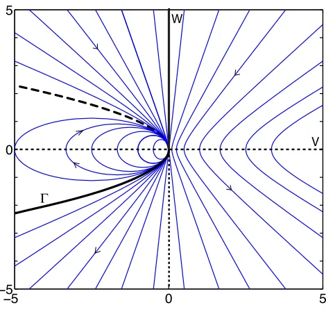
κ < 0. If κ = 0, this is simply the parabola v =−w2. The (v, w) phase portrait is shown in
Figure 4.1.
(3) The solution to (4.3) with initial conditionsv(0) =v0, w(0) =w0 is
v(t) = v0
q(t), w(t) =
w0−v0t
q(t) (4.5)
with q(t) = 1 + 2w0t+v0t2.Since q(t) is quadratic in time, then the smallest positive zero (if any exists) will be the time at which∇ϕ= (v, w) develops a finite time singularity. The zeros
of q(t) are
t±(v0, w0) =
w0
v0 ± 1
v0
+
w20+v0, ifv0 '= 0
−21 w0
ifv0 = 0, w0 '= 0.
(4.6)
This results in four different cases. (a) If v0>0,thent−<0< t+.
(b) If −w02≤v0 ≤0,and w0 <0 then 0< t+≤t−.
(c) If −w2
0 ≤v0≤0,andw0 >0,then t± <0.
(d) If v0<−w20,then t± are complex.
In cases (a) and (b), the phase portrait is unbounded and involves finite time blow-up;
−5 0 5
−5
0
5 W
V
'
Figure 4.1: Phase portrait for system (4.3).
t → ∞; the roots t± are either complex or negative. Since blow-up of ∇ϕ on characteristics
is determined by these solutions, precise conclusions can be drawn for shock formation based solely on the gradient of the initial data ∇ϕ0 = (v0, w0). Let Γ be the union of the curve
{(v0, w0) : v0 = −w02, w0 < 0} with the positive w0 axis {(0, w0) : w0 ≥ 0}, and let D be the region to the right of Γ in the (v, w) plane. Then finite time shock formation can be
characterized for the initial value problem on the entire plane
ϕt+zϕx+ (ϕ(ϕ−1))z = 0, −∞< x, z <∞, t >0 (4.7a)
ϕ(x, z,0) = ϕ0(x, z) − ∞< x, z <∞. (4.7b)
with the following theorem.
develops a singularity: sup(x,z)|∇ϕ(x, z, t)| →∞ as t→t∗−in finite time t∗ given by
t∗= inf{t+(∇ϕ0(x, z)) :∇ϕ0(x, z)∈ D} (4.8)
Proof: If (v0, w0) ∈ D, then t+ > 0 is real, and t− is either negative or greater than t+. Individual contours evolve according to (3.2), and the normal (v, w) =∇ϕ evolves along
char-acteristic curves (on which ϕ is constant) according to (4.3). Consequently, the singularity
|∇ϕ| → ∞ develops at the smallest value oft+,evaluated on the initial data, as in (4.8). The theorem can be interpreted by dividingDand its complement in the (v0, w0) plane into four regions in which the behavior of the characteristics acts differently.
(i) v0 > 0, w0 > 0. In this case, the trajectory lies on the hyperbola given by (4.4) with
κ =κ0 <0. From Figure 4.1, the phase portrait clearly shows that |∇ϕ|=|(v, w)| decreases, meaning contours are spreading out. Once the trajectory crosses thev-axis at t=w0/v0 from (4.5), contours of ϕbecome vertical in (x, z), tip over, and begin to compress as ∇ϕ= (v, w)
has now entered the fourth quadrant of the phase portrait.
(ii) v0 >0, w0 < 0. Here, |∇ϕ|=|(v, w)|increases corresponding to a compressing of the contours of ϕ. Eventually, v(t) and w(t) blow-up in a finite amount of time, given by the
positive zero ofq(t) in (4.6). At this time,ϕ(x, z, t) develops a jump discontinuity at this value
of (x, z).
Cases (i) and (ii) together show that |∇ϕ| → ∞ along the characteristic as t increases if
ϕx=v >0 initially. Physically, a region of more small particles has developed below a region
with a higher concentration of large particles; subsequent segregation sharpens the profile ofϕ,
eventually forming a shock.
positive zeros ofq(t) in (4.6). Here, the contours always have a negative slope as they get closer
together, quickly forming a shock.
(iv) In the remaining portion of the (v, w) plane for whichw0>−√v0, v0<0, the contours may switch from having negative slope (if w0 < 0) to a positive one (when w > 0). In this case, |∇ϕ| increases before decreasing to zero, corresponding to an initial compression of the
contours, before they expand. However if w0 >0, then|∇ϕ| decreases monotonically to zero. In other words, the contours start expanding and continue to do so. Note that anywhere in this region |∇ϕ|= |(v, w)| → 0 as t → ∞, meaning (ϕx, ϕz) → (0,0), or in other words, the
solution ϕ(x, z, t) is smoothening out and tending toward a constant.
4.2
Shock formation example
The phase portrait and subsequent analysis of the shock formation time given by (4.6) and (4.8) from Theorem 4.1.1 paint a complete picture of intetrior shock formation for smooth initial data. Consider the following initial data:
ϕ0(x, z) =±0.1 tan
!π
2z
"
+1
2 ±x. (4.9)
This initial condition represents initial data from each of the four quadrants of the phase portrait, depending on the choices of sign, which represent each of the four cases (i-iv) of§4.1.
The initial gradient
∇ϕ0 = (v0, w0) =
!
±1,±0.1π
2 sec2
!π
2z
""
(4.10)
is used to find the solution along each trajectory (4.5), as well as the blow-up time (4.8). (i) In the first case, the gradient is positive in both the v and w directions, meaning the
positive sign is chosen in both components of (4.10). As described in case (i) from §4.1 the
interior contours initially expand and have a negative slope in the (x, z) plane. At
each contour becomes vertical, tips over and the slope of the contour becomes positive as ∇ϕ
crosses thev-axis and enters the fourth quadrant. The first slope to do so is the slope given by
the minimum value oftin (4.11); this occurs atz= 0 witht≈0.157. Now that the trajectories
have entered the fouth quadrant, they compress until a shock forms. Using (4.6) and (4.8), the shock formation time becomes
t∗ = inf
z
,
t+(z) = 0.1
π
2 sec2
!π
2z
"
+-!0.1π
2 sec2
!π 2z ""2 + 1 . . (4.12)
The infimum is actually achieved at the minimum value, which again occurs atz= 0 at a time
oft∗ ≈1.169. Thus, an interior shock has first formed at this timet∗ at the point (x, z) = (0,0).
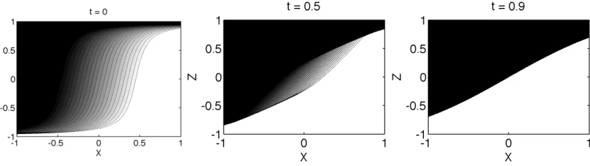
(ii) In this case, contours that initially start out with all positive slope in (x, z) and an
initial gradient pointing toward the fourth quadrant. Here, contours simply compress until they form a shock, which occurs rapidly using the initial data in this example. Fourth quadrant initial data are represented by taking the positive sign forv0 and the negative sign forw0 from (4.10). The blow-up time now becomes
t∗ = inf
z
,
t+(z) =−0.1
π
2 sec2
!π
2z
"
+-!0.1π
2sec2
!π 2z ""2 + 1 . . (4.13)
With an unbounded x domain, the infimum occurs as x → ∞, z → ±1, yielding t∗ = 0.
However, using a bounded domain −1≤x, z≤1, the infimum occurs at x=±1, z ≈ ±0.874,
giving a blow-up time of t∗ ≈ 0.121. A stable shock has completely formed leaving a fully
segregated material at the maximum value of (4.13); this is whenz= 0 at a time oft∗ ≈0.855.
In other words, shocks forms quickly at the outer ends of the domainx=±1 where the initial
gradient is the steepest, and move in toward and meet at the middle at x = 0, resulting in
complete segregation with large particles above small ones.
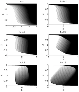
(iii) Taking the negative sign for both v0 and w0 puts the initial data in the third quadrant of the phase portrait. Where the gradient is steep initially, with x and z near ±1, the initial
hand, in areas of shallow initial gradient, the initial data falls to the left of Γ where trajectories head toward the origin and contours expand. The initial data in the third quadrant that lie on Γ is given by v0 = −w02. Solving this equation using (4.10) yields z0 ≈ ±0.741 which subsequently gives x0 ≈ ∓0.732. In other words, in areas where |x0| ! 0.732 a shock forms, and no shock forms from initial data in the complementary region. The initial shock formation time is found using the same procedure as case (ii), yielding the same values t∗ = 0 on an
unbounded domain, andt∗ ≈0.121 on the domain−1≤x, z≤1. Unlike case (ii), a shock does
not completely segregate small and large particles, and instead the interior mixing region after an initial compression until t=w0/v0 ≈0.157 tilts over and expands.
(iv) In the simplest of the four cases where v0 uses the negative sign in (4.10) and w0 the positive, contours expand as|∇ϕ| →0. As seen from Figure 4.1 the gradient remains bounded
(and decrese monotonically) as trajectories head toward the origin. The only shocks that form are the shocks propagating inward from the boundary (not interior shocks).
This example, with initial ϕ0 given by (4.9) and initial gradient ∇ϕ0 by (4.10) encompasses all the possible outcomes for shock formation using (4.1) with u(z) =z and f(ϕ) = ϕ(ϕ−1).
The initial data determines not only if a shock forms, but at what specific time the shock will form. Analysis of the the third quadrant distinguishes between initial data where interior shocks form, and initial data where a smooth mixing region occurs. The time to complete segregation is found in the second quadrant. The behavior of (4.1) is well understood from analysis of the four cases in this example, and is verified using numerical simulations in§4.3.
4.3
Shock formation simulations
The results from §4.2 are illustrated in the first set of numerical simulations in this section.
Subsequent simulations are just to verify and confirm the behavior found in§4.1 and§4.2. The
finite difference code, written initially by Rowe [53] and modified for these specific examples, employs an upwind differencing in x, and a first order Godunov method inz with an explicit
plotted on the smaller, bounded domain−1≤x≤1, −1≤z≤1. The smaller domain means
that time can be computed up to t = 2 so that effects of the lateral boundaries at x = ±3
are not noticed. Boundary conditions at z = ±1 ensure that particles do not penetrate the
boundaries. These conditions
ϕ(x,−1) = 1, ϕ(x,1) = 0 (4.14)
physically equate to a layer of all small particles at the bottom and a layer of all large particles at the top (despite an actual system having a free surface at the top) so that mixing and segregation do not occur beyond the boundaries. These conditions are consistent with no-flux boundary conditions f(ϕ) = 0, but are easier to use in the numerical code. The boundary
conditions (4.14) actually amount to a horizontal stationary shock if ϕ = 0 next to z = −1
(and respectivelyϕ= 1 next toz= 1). The horizontal, stationary shock remains until the first
small particle reaches the bottom (or, respectively, until the first large particle reaches the top
z= 1). When this occurs, a boundary shock forms and propagates toward the interior. These
shocks are not interior shocks characterized in §4.1 and§4.2, but rather just layers of small or
large particles accumulating at the bottom or top.
The first set of four simulations uses the initial data given by (4.9) and (4.10) from §4.2.
Each simulation corresponds to one quadrant of Figure 4.1 and to a corresponding case (i)-(iv)
in§4.2.
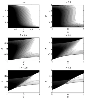
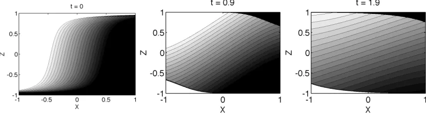
In Fig. 4.2, ∇ϕ0 = (v0, w0) is in the first quadrant. Corresponding to case (i) from §4.2, contours of ϕ initially spread out, and then steepen as the normal∇ϕ rotates clockwise. As
the contours reach the boundaries z=±1,a layer of small particles grows from z=−1,with
a sharp shock wave interface propagating upwards. Similarly, a layer of large particles grows from z = 1, led by a shock wave propagating downwards. Between these shocks, contours
continue to rotate, until ∇ϕ enters the fourth quadrant. The first contour whose slope enters
into the fourth quadrant is the contour atz= 0 and the contour becomes vertical att≈0.157