©
DOI: 10.1534/genetics.104.033910
Model Selection in Binary Trait Locus Mapping
Cynthia J. Coffman,*
,†R. W. Doerge,
‡,§Katy L. Simonsen,
‡Krista M. Nichols,**
Christine K. Duarte,
††,‡‡Russell D. Wolfinger
‡‡and Lauren M. McIntyre
†,§,§§,1*Institute for Clinical and Epidemiological Research Biostatistics Unit, Durham VA Medical Center (152), Durham, North Carolina 27705, †Department of Biostatistics and Bioinformatics, Duke University Medical Center, Durham, North Carolina 27710,
‡Department of Statistics, Purdue University, West Lafayette, Indiana 47907-2068,§Department of Agronomy, Purdue University, West Lafayette, Indiana 47907,§§Computational Genomics, Purdue University,
West Lafayette, Indiana 47907,**Washington State University, School of Biological Sciences, Pullman, Washington 99164,††Department of Statistics, North Carolina State University,
Raleigh, North Carolina 27695 and‡‡SAS Institute, Cary, North Carolina 27513
Manuscript received July 23, 2004 Accepted for publication March 17, 2005
ABSTRACT
Quantitative trait locus (QTL) mapping methodology for continuous normally distributed traits is the subject of much attention in the literature. Binary trait locus (BTL) mapping in experimental populations has received much less attention. A binary trait by definition has only two possible values, and the penetrance parameter is restricted to values between zero and one. Due to this restriction, the infinitesimal model appears to come into play even when only a few loci are involved, making selection of an appropriate genetic model in BTL mapping challenging. We present a probability model for an arbitrary number of BTL and demonstrate that, given adequate sample sizes, the power for detecting loci is high under a wide range of genetic models, including most epistatic models. A novel model selection strategy based upon the underlying genetic map is employed for choosing the genetic model. We propose selecting the “best” marker from each linkage group, regardless of significance. This reduces the model space so that an efficient search for epistatic loci can be conducted without invoking stepwise model selection. This procedure can identify unlinked epistatic BTL, demonstrated by our simulations and the reanalysis ofOncorhynchus mykiss experimental data.
S
TATISTICAL methods for mapping single genes for that estimates the effect for all markers, thus avoiding continuous and binary traits in experimental popula- the testing and model selection issues.tions have advanced significantly in the past few years One approach for reducing the dimensionality of the
(LanderandBotstein1989;HaleyandKnott1992; model space is to locate all QTL that are significantly
Zeng1994; Satagopan et al.1996; Xu 1996; Xu and associated with the trait, using single-QTL methods, and
Atchley1996;YiandXu2000;McIntyreet al.2001; then build the multiple-QTL models using only the QTL
YiandXu 2002). Single-gene QTL models have been selected in the single-gene analysis (Kao et al. 1999). expanded to encompass multiple-QTL mapping prob- When all QTL are additive, single-marker analysis is a lems by using cofactors or additional markers (Jansen reasonable strategy for identifying QTL (Coffmanet al.
1993;Zeng1994;Xu2003). Multiple-QTL models have 2003). However, epistasis can alter the trait in a manner been developed for both continuous and binary traits that may be difficult to predict (Doerge 2001), thus
(Sillanpa¨a¨ and Arjas 1998; Kao et al. 1999; Zenget further complicating the model fitting and selection
al.2000;JanninkandJansen2001;SenandChurchill process.Carlborget al.(2000) proposed a method for 2001;CarlborgandAndersson2002;YiandXu2002; simultaneous mapping of pairwise interacting QTL. In
Xu2003) and for discrete traits with multiple observa- addition,CarlborgandAndersson(2002) proposed a tion classes (Yiet al.2004). When attempting to identify forward selection strategy that incorporates a random-multiple QTL for a trait, model selection is a key issue ization test to identify epistatic QTL. Unfortunately, this as the number of possible models quickly becomes large. approach will miss pairs of loci that are epistatic without In most analyses, the enumeration of all QTL models for a contributing main effect.Hollandet al.(2002) per-a dper-atper-a set is possible only when the number of mper-arkers is formed a pairwise grid search to identify potential epi-limited. An exception is a recent method (Xu 2003) static loci and then include the most significant pairs in the “best” single-gene model via a forward stepwise
procedure. Yi and Xu (2002) proposed a Bayesian
1Corresponding author:Department of Agronomy, 915 W. State St.,
method to map multiple QTL with pairwise locus epista-Purdue University, West Lafayette, IN 47907.
E-mail: [email protected] sis.SenandChurchill(2001) also presented a
ian analysis that implements a strategy similar to that segregation and linkage analysis. The concept of incom-plete penetrance is important, as it underscores the
of Jansen(1993), where the QTL problem is divided
complexity encountered in analysis of binary traits. into two pieces, detection and then localization. While
As an adaptation of the model in human genetics, and all of these approaches have a common goal, the
com-extension of previous work in experimental populations plexity and computational intensity of many of these
(McIntyreet al.2001), we propose a method to detect
approaches make them difficult to implement.
Further-and estimate multiple binary trait loci (BTL). We focus more, stepwise procedures and pairwise searches do not
on the case where penetrance is incomplete and the investigate the entire model space and these approaches
population structure is a backcross or F2from two inbred
have been shown to fail to identify all possible effects
parents. Using the biological information in the linkage in different applications (Harrell2001;Burnhamand
groups, the model space is reduced by choosing the
Anderson2002).
best marker in each linkage group. Consequently, all Searching through the potential models to identify
possible models can be enumerated and stepwise selec-the best model is an active area of statistical research
tion procedures are avoided, which in turn eliminates
(Harrell2001;BurnhamandAnderson2002).
Sev-the need for computationally intensive model space ex-eral common criteria are used to judge and compare
ploration. We use a general probability model based on models to select the best model. Due to the large
num-classical transmission genetics to develop a likelihood ber of models that may be examined in these analyses,
for the binary phenotype (Simonsen2004) to estimate issues of model selection bias and uncertainty should
recombination and penetrance for multiple BTL under be addressed (Burnham andAnderson2002). In the
complex genetic models for an experimental popula-method described by Jansen(1993), the Akaike
infor-tion. Regression models are fitted on the basis of this mation criterion (AIC) was used for model selection.
likelihood (HaleyandKnott1992;Jansen1992;
Jan-Broman and Speed (2002) reviewed different model
senandStam1994;Whittakeret al.1996;Thompson
selection criteria for QTL analysis and proposed a
crite-1998), using a cell means model parameterization rion that is a modification of the Bayesian information
rather than the factor effects parameterization (Kutner
criterion (BIC) (Schwarz1978).Sillanpa¨a¨and
Coran-et al.2004). The parameterization in terms of the cell
der (2002) gave a general review of model selection
means clarifies the identification of epistatic loci. criteria and advocated the Bayesian idea of model
aver-Using simulated data, AIC (Akaike 1973) and BIC aging. Others are working on modifications of these
(Schwarz1978) model selection criteria are employed
criteria to improve their performance in the QTL setting
and compared for a limited number of markers as well as (Ball2001;Bogdanet al.2004;Siegmund2004).
How-in the context of a genome scan. A new SAS procedure, ever, these criteria have not been specifically evaluated
PROC BTL, has been developed and is freely available for binary traits.
by request (http:www.genomics.purdue.edu/services/ In genetic experiments, binary traits often occur
software/btl). PROC BTL includes model selection for when considering characteristics related to
susceptibil-a wide rsusceptibil-ange of model selection criterisusceptibil-a susceptibil-and implements ity/resistance, sterility/fertility, and mortality/survival.
all of the standard model selection techniques including
SenandChurchill (2001) examined binary traits
us-the one proposed here. Using PROC BTL, we present ing a generalized linear model framework. YiandXu
a reanalysis ofOncorhynchus mykiss(rainbow or steelhead
(2000) proposed a Bayesian method for complex binary
trout) data where single-marker associations of the bi-traits under the threshold model and later extended
nary trait, resistance to Ceratomyxa shasta(a myxozoan this method to map multiple QTL with pairwise locus
parasite) (Nichols et al. 2003), suggest that multiple epistasis for binary traits (YiandXu 2002). Kilpikari
loci may be associated with the resistance. We also find
and Sillanpa¨a¨ (2003) present a multilocus Bayesian
evidence for epistatic effects. approach for association mapping that can be used for
binary traits under the threshold or liability model. The threshold model is an important quantitative genetic
METHODS model. However, the underlying threshold distribution
is unobserved (Falconer and Mackay 1996; Lynch A probability model: We denote individual genetic
andWalsh1998), presenting challenges in specifying markers by Mi and BTL by Gi, where i indicates the
the functional form of the threshold model. BTL in map order. We assume a map based onkBTL
In the human genetics literature, binary traits (disease andkmarkers (M1G1M2G2· · ·MkGk). The complete
status) are often parameterized in terms of the pene- genotype for all loci is denoted M for markers and G trance as well as the physical distance. This model forma- for BTL, and the possible values are described below. tion has been routinely employed for segregation and For a backcross (BC) or F2population of diploid
tion withkloci, there are 2kdistinct marker classes (i.e., Trait values can be modeled in a variety of ways, and
possible values for M) and 2k distinct BTL genotypes it is useful to consider the penetrancepin the context
(i.e., possible values forG), giving a total of 4kpossible of standard ANOVA models. For example, consider a
combinations of genotypic marker classes (M,G). In an backcross withk⫽ 2. The penetrance parameters are F2population with phase unknown, there are 3kdistinct pgj, wheregj ⫽ {11, 12, 21, 22}. Suppose the first digit
marker classes forMand 3kdistinct BTL genotypes for
of gj is s and the second digit is t. The factor effects
G, resulting in a total of 9k possible combinations of
parameterization would bepgj⫽ ⫹ ␣s⫹ t⫹(␣)st,
marker classes and genotypes for (M,G). The number where␣andare the main effects at the two loci and of distinct marker classes or genotypes is represented (␣) represents the interaction or epistatic effect and byKfrom this point forward (i.e.,K ⫽ 2kfor BC and
0ⱕ pgj, ⱕ 1. The corresponding cell means model
K⫽ 3kfor F
2). parameterization ispg
j⫽ st, where thestare (a
func-As in Simonsen (2004), we label and order the K tion of) the cell means. These two model
parameteriza-possible genotypes of markers or BTL as if the genotypes tions are equivalent (Kutneret al.2004). In the factor were numerals with one digit per locus, in ascending effects parameterization, absence of epistasis is indi-order. The digit 1 represents the homozygote 1/1 geno- cated by (␣)
st⫽0 and is equivalent to the constraint
type at that locus, 2 is the 1/2 or 2/1 heterozygote, and in the cell means model ofp
11⫺ p12 ⫽ p21⫺ p22(see
3 is the 2/2 homozygote. A genotype forkloci is then Figure 2a). If only locus 1 contributes to the trait, the akdigit number. Thus, withk⫽2, a backcross hasK⫽ factor effects model constraint is
t⫽(␣)st⫽0 while
4 possible types {11, 12, 21, 22}, whereas an F2hasK⫽ the cell means model constraint isp11⫽p
12andp21⫽
9 possible genotypes {11, 12, 13, 21, 22, 23, 31, 32, 33}. p22. Similarly, if only locus 2 is involved, the factor effects We label these K values m1, . . . , mK or g1, . . . , gK, model constraint is␣
s⫽(␣)st⫽0 and the cell means
depending on whether they represent markers or BTL, model constraint is p
11 ⫽ p21 and p12 ⫽ p22. Epistasis
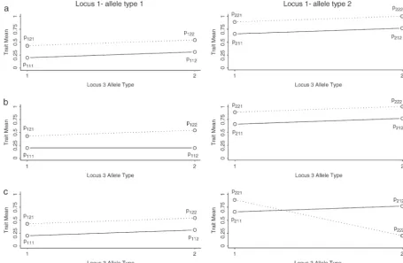
respectively. The probability distribution ofMorGspec- can be presented as a modification of the expected ifies the probabilities of each of theseKvalues and thus segregation ratio with fewer than expected phenotypic can be written in a vector of lengthKin the order given. classes observed (HartlandJones 2001). Therefore, The joint probability distribution of (M,G) can be writ- the cell means model provides a convenient way of ten as aK⫻KmatrixPr(M,G), where the rows index thinking about genetic models, as epistasis is easily de-the marker classes and de-the columns index de-the BTL geno- fined as equivalence among penetrance parameters (see types. The (i,j)th entry of this matrix represents Pr(M⫽ Figures 2, b–d, and 3).
mi,G⫽gj), wheremi andgj each take on theKpossi- Simonsen (2004) details the methods for generating
bilities described above. All matrices and vectors
refer-the probability model fork BTL in matrix form. The ring to genotypes assume this ordering and indexing.
joint probabilities of the BTL genotypes (G), marker The recombination rate,ri, is the probability that an types (M), and the trait (Y), denotedPr(Y,M,G), can
exchange of genetic material (crossover) occurs
be-be expressed in terms ofr,, andpand generated for tween the BTLGiand the marker Mi, wherei ranges
k BTL for a specified experimental design. Standard from 1 tok, whereri⫽0 indicates complete association
assumptions such as no selection, interference, or muta-and ri ⫽ 0.50 indicates no association between the
tion are made. As an example, the joint probability marker and the BTL. Similarly, the rate of
recombina-distribution of a BC fork⫽2 is shown in Table 1. The tion between markers,i, is the probability that an
ex-joint probability of every combination of marker and change of genetic material occurs between markerMi
BTL genotype,Pr(M,G), is computed using the recom-andMi⫹1, whereiranges from 1 tok⫺1. If the marker
bination probabilitiesandr. The matrix for the joint map is assumed known, then theiare fixed.
probability of trait, marker, and BTL is then computed The probability of observing the binary trait is
speci-by matrix multiplication Pr(Y, M, G) ⫽ Pr(M, G) ⫻ fied byKpenetrance parameters,pj, which are Bernoulli
Diag(p), since probabilities representing the probability that a binary
traitYis present given a specific BTL genotypej(McIn- Pr(Y⫽1,M⫽m
i,G⫽gj)⫽Pr(Y⫽1|G⫽j)Pr(M⫽mi,G⫽gj)
tyreet al.2001). The vectorpwith entriespj⫽Pr(Y⫽
⫽[Pr(M,G)]i,j⫻pj.
1|G ⫽ gj) is of length K, and its jth entry, pj, is the
penetrance parameter for thejth genotype,gj, wherej
The joint probability of traits and markers only is used indexes the possible genotypes in the order explained
for likelihood calculations as described in the next sec-above. To emphasize the relationship between the
geno-tion. This vector of probabilities is computed asPr(Y, type and the penetrance the notationpgjmay be used
M)⫽ Pr(M, G)⫻ p, where the matrix multiplication as well as the abovepj. Including a penetrance
parame-accomplishes the necessary sum over possible geno-ter for each genotype is convenient for visualizing the
types. Itsith entry is impact of various genetic models on the parameter
space and is a common tool in human genetics (Ott
Pr(Y⫽1,M⫽mi)⫽
兺
Kj⫽1
Pr(Y⫽1,M⫽mi,G⫽gj)
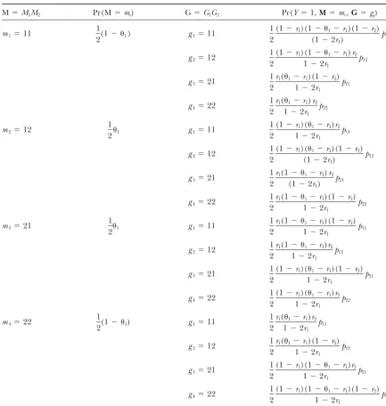
TABLE 1
Expected trait distributions for binary traits in a backcross with two markers and
two loci for linkage mapM1G1M2G2
M⫽M1M2 Pr(M⫽mi) G⫽G1G2 Pr(Y⫽1,M⫽mi,G⫽gj)
m1⫽11
1
2(1⫺ 1) g1⫽11
1 2
(1⫺r1)(1⫺ 1⫺r1)(1⫺r2)
(1⫺2r1)
p11
g2⫽12
1 2
(1⫺r1)(1⫺ 1⫺r1)r2
1⫺2r1
p12
g3⫽21
1 2
r1(1⫺r1)(1⫺r2)
1⫺2r1 p21
g4⫽22
1 2
r1(1⫺r1)r2
1⫺2r1 p22
m2⫽12
1
21 g1⫽11
1 2
(1⫺r1)(1⫺r1)r2
1⫺2r1 p11
g2⫽12
1 2
(1⫺r1)(1⫺r1)(1⫺r2)
(1⫺2r1)
p12
g3⫽21
1 2
r1(1⫺ 1⫺r1)r2
(1⫺2r1) p21
g4⫽22
1 2
r1(1⫺ 1⫺r1)(1⫺r2)
1⫺2r1
p22
m3⫽21
1
21 g1⫽11
1 2
r1(1⫺ 1⫺r1)(1⫺r2)
1⫺2r1
p11
g2⫽12
1 2
r1(1⫺ 1⫺r1)r2
1⫺2r1 p12
g3⫽21
1 2
(1⫺r1)(1⫺r1)(1⫺r2)
1⫺2r1
p21
g4⫽22
1 2
(1⫺r1)(1⫺r1)r2
1⫺2r1 p22
m4⫽22
1
2(1⫺ 1) g1⫽11
1 2
r1(1⫺r1)r2
1⫺2r1 p11
g2⫽12
1 2
r1(1⫺r1)(1⫺r2)
1⫺2r1 p12
g3⫽21
1 2
(1⫺r1)(1⫺ 1⫺r1)r2
1⫺2r1
p21
g4⫽22
1 2
(1⫺r1)(1⫺ 1⫺r1)(1⫺r2)
1⫺2r1
p22
Recombination between markers M and BTLG is denoted by r and recombination between markers is denoted by . Penetrances are pgj⫽Pr(Y⫽1|G⫽gj). Genotypes of the fixed (parental) haplotypes are omitted.
For a k ⫽ 2 BTL BC population, the four possible
⫽
兺
Kj⫽1
Pr(Y⫽1|G⫽gj)Pr(M⫽mi,G⫽gj)
(nonfixed) marker allele combinations are m1 ⫽ 11, m2 ⫽ 12, m3 ⫽ 21, m4 ⫽ 22, and the matrix rows are
⫽
兺
Kj⫽1
[Pr(M,G)]i,j⫻pj.
given in that order (see Table 1); columns index BTL genotypes in a similar order. Thus row 1 in the matrix Although the focus of this work is on backcross and
Pr(Y,M,G) is
F2 populations, the matrix Pr(M, G) can be obtained
for any mating scheme. The probability distribution for 1 2(1⫺2r1)
[(1⫺r1)(1⫺ 1⫺r1)(1⫺r2)p11 (1⫺r1)(1⫺ 1⫺r1)r2p12
a generation of offspring can be calculated from the
probability distributions for the parental generation, r
1(1⫺r1)(1⫺r2)p21 r1(1⫺r1)r2p22].
through appropriate matrix operations. By repeating
Likelihood:Using the notation above, the likelihood
this process any scheme can be derived back to known
L(r,,p)⫽ Pr(Y⫽y,M⫽m|r,,p). The resulting system of equations is linear inpand and nonlinear in r. Since there are K equations and This likelihood can also be written in terms of the
K⫹ kunknowns, the system is underdetermined. For marker class means, as follows.
any fixedr, however, there is a unique and easily ob-The expected marker class means are denoted by the
tained solution forp, and, furthermore, the values are vectorwhoseith entry, i, is the marker class mean
subject to constraints, namely 0 ⱕ ri ⱕ 0.5 and 0 ⱕ
for marker classi, namely
pgjⱕ1. We use a grid search to step through the interval
of possible r values to obtain sets of solutions for p. i ⫽Pr(Y⫽ 1|M⫽ mi)⫽
Pr(Y⫽1,M⫽mi)
Pr(M⫽mi) In some cases, solutions do not satisfy the biological
constraint 0ⱕ pˆgjⱕ 1 for allgjand can be discarded,
or simply if a filter on the resulting estimates is desired. In other
situations, the correct values of some penetrances may
Pr(Y⫽1,M⫽mi)⫽ iPr(M⫽mi).
be known or separately estimable from previous experi-The component of the likelihood for a single observa- mental generations. In these cases estimates can be fur-tion withY⫽1 andM⫽miis theith entry of the vector ther constrained. For example, if parental penetrances
Pr(Y ⫽ 1,M). Since Pr(Y ⫽ 0|M ⫽ mi)⫽ 1⫺ i, we are known, the values of rˆ and pˆ that minimize the
havePr(Y⫽ 0,M⫽ mi)⫽(1 ⫺ i)Pr(M⫽ mi). Note distance between the known values of the parental
pene-that is a function of r, , and p, while Pr(M) is a trances and their estimates can be chosen. Other possi-function ofonly. Therefore, the likelihood for a single ble solutions to this problem exist; for example,
nonlin-observation from marker classiis ear programming methods may be applied. We initially
explored applying nonlinear programming (NLP) tech-niques; however, estimation for k loci was not easily
L(r,,p)⫽
冦
iPr(M⫽ mi), Y⫽ 1 (1 ⫺ i)Pr(M⫽mi), Y⫽ 0.implemented.
Premodeling strategy:Generally, mapping data
con-Suppose in a given sample there areniindividuals in
sist of a set of markers and a trait evaluation for each marker class i, of whom zi exhibit Y⫽ 1, and ni ⫺ zi
individual in the experimental population. The number exhibitY⫽0. Then the likelihood can be written as a
of BTL that can be fit to the data depends on the sample product over marker classes:
size (i.e., the degrees of freedom). If the set of markers
L(r,,p)⫽
兿
K
i⫽1
(iPr(M⫽mi))zi((1⫺ i)Pr(M⫽mi))ni⫺zi(1) is relatively large, as is generally the case, enumerating all possible models becomes impossible, and we need some methodology for reducing the model space. We ⫽
兿
Ki⫽1 zi
i(1⫺ i)ni⫺zi(Pr(M⫽mi))ni. (2)
propose to limit the model space explored by choosing one marker per linkage group. Another strategy for Maximum-likelihood estimates for marker class
reducing the model space is to limit multiple-marker
means:Using this likelihood, the maximum-likelihood
models to only markers that are significantly associated estimates (MLEs) for the marker class means can be
with the trait on the basis of single-locus models (Kao
obtained by maximizing model 1 to obtain estimates of
et al.1999;CarlborgandAndersson2002). However, the binomial proportionsˆi⫽ zi/nifori⫽ 1 . . .K.
this strategy might miss markers without strong main The marker class meansiare easily estimated from
effects that are otherwise involved in epistasis. Another the data. To estimate penetrancepand recombination
strategy is to examine all possible pairs of loci (Holland
r, we exploit the relationship betweenpand. Let⍀ ⫽
et al.2002; Yiand Xu 2002) to reduce the chance of Diag(Pr(M)) such that⍀⫺1⫽Diag(1/Pr(M⫽m1), . . . ,
missing a locus with primarily epistatic effect. While 1/Pr(M⫽mK)). ThenPr(G|M)⫽ ⍀⫺1Pr(M,G) so that
it is possible to look at all possible pairs of markers, Pr(G|M)⫺1⫽Pr(M,G)⫺1⍀can be calculated. In terms
examining all possible triplets and quadruplets quickly of this quantity, the relationship between p and is
becomes impractical. Additionally, significant model se-thus
lection bias and uncertainty is introduced (Burnham
⫽Pr(Y⫽1|M)⫽ Pr(G|M)⫻ p, andAnderson2002;Bogdanet al.2004).
To avoid stepwise procedures and selection methods so that
based upon pairwise relationships it has been proposed
p⫽[Pr(G|M)]⫺1⫻.
that the relationships among predictor variables can be exploited to reduce model space (Harrell2001). This givespas a function ofr,, and. If the marker
Fortunately, markers have an inherent relationship among map is known [and hencePr(M) is known],pis a
func-themselves based on genetic distance and form groups tion of onlyrand.
of correlated covariates known as linkage groups. By
Estimation:To estimate recombination (r) and
pene-selecting the best marker (or interval) from each linkage trance (p) parameters the invariance property of MLEs
group, the dimensionality of the problem is greatly re-can be invoked (CasellaandBerger1990). Thus
duced. The criteria for choosing the best among the markers for a linkage group are also possible to explore.
pˆ ⫽[Pr(G|M)]⫺1|
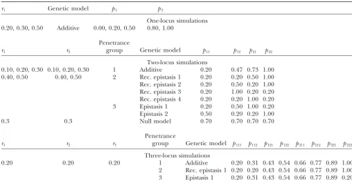
TABLE 2
Simulation conditions: simulation 1
r1 Genetic model p1 p2
One-locus simulations 0.20, 0.30, 0.50 Additive 0.00, 0.20, 0.50 0.80, 1.00
Penetrance
r1 r2 group Genetic model p11 p12 p21 p22
Two-locus simulations
0.10, 0.20, 0.30 0.10, 0.20, 0.30 1 Additive 0.20 0.47 0.73 1.00
0.40, 0.50 0.40, 0.50 2 Rec. epistasis 1 0.20 0.20 0.50 1.00
Rec. epistasis 2 0.20 0.50 0.20 1.00 Rec. epistasis 3 0.20 1.00 0.20 0.20 Rec. epistasis 4 0.20 0.20 1.00 0.20
3 Epistasis 1 0.20 0.50 1.00 0.20
Epistasis 2 0.50 0.20 0.20 1.00
0.3 0.3 Null model 0.70 0.70 0.70 0.70
Penetrance
r1 r2 r3 group Genetic model p111 p112 p121 p122 p211 p212 p221 p222
Three-locus simulations
0.20 0.20 0.20 1 Additive 0.20 0.31 0.43 0.54 0.66 0.77 0.89 1.00
2 Rec. epistasis 1 0.20 0.20 0.43 0.54 0.66 0.77 0.89 1.00 3 Epistasis 1 0.20 0.31 0.43 0.54 0.66 0.77 0.89 0.20
One-locus simulation conditions: one marker (M1) and one BTL (G1), wherer1is the recombination betweenM1andG1,p1
is the penetrance of genotypeG1G1andp2is the penetrance of genotypeG1G2. Two-locus and three-locus simulation conditions:
two markers (M1M2) and two BTL (G1G2) and three markers (M1M2M3) and three BTL (G1G2G3), respectively, whereriis the
recombination betweenMiand Gi, iis the recombination betweenMiand Mi⫹1, three values foriwere simulated for each
combination of parameters (low to no linkage, medium linkage, and high linkage), andpgjis the penetrance of genotypegj.
For simplicity, we choose the marker with the lowest ple AIC (Sugiura1978), denoted AICc, is available to
be used when the ratio of sample size (n) to number
P-value. However, if there are unequal amounts of
miss-ing data, it would be possible to include the amount of of parameters (p) is small (i.e., ⬍40) (Burnham and
Anderson2002). In contrast, dimension-consistent
cri-missing data as a criterion for selection. AIC and BIC
could also be used in this context. By choosing a marker teria (e.g., BIC) assume that one of the models is the true model and is not based in the theory of optimization. in each linkage group without regard to the
“signifi-cance,” epistatic loci that show little or no main effect Implicit in the assumption that one of the models is the “true” model is that the “truth” is of fairly low dimension can be detected. The reduction in overall
dimensional-ity reduces the number of models. Thus, the genetic (Burnham and Anderson 2002). Asymptotically the
BIC will select the true model with probability 1, if that model space can be explored without the assistance of
complex searching algorithms and the overall model model is in the set. The goal of these criteria (AIC or AICcand BIC) is to allow for ranking and comparison
bias and uncertainty are reduced.
Model selection: To select a model or set of models of models to separate models that are equally useful
from those that are clearly not useful (Burnhamand from among a number of models, standard model
selec-tion criteria, AIC (Akaike 1973) and BIC (Schwarz Anderson2002).
Whichever criterion is applied, models or sets of mod-1978), are often employed. Mallow’sCp(Mallow1973)
is another commonly used criterion that tends to select els need to be delineated for evaluation. When large numbers of models are evaluated, model uncertainty the the same models as AIC (QuinnandKeough2002).
We explored the behavior of Cp in this context and and parameter estimation bias are likely outcomes
(BurnhamandAnderson2002). Byselecting one marker
found it to be very similar to AIC; therefore, we did not
include Mallow’sCpin our formal evaluation of model per linkage group, regardless of whether that model is
significant, the full set of hierarchical regression models selection criteria.
AIC is a very general methodology based on the theory can be fit. This eliminates the need for stepwise proce-dures. For example, if there are 10 linkage groups and of optimization where the goal is to select the best
sam-and adjacent to a BTL with one marker not linked to any BTL (see Figure 1). Since the objective is to study the impact of the genetic model, a large sample size was chosen. When only one BTL locus is truly present (k⫽1), there is no epistasis.
When more than one locus is involved, the set of genetic models explored in a simulation study is essen-tially infinite. For convenience we categorized the ge-netic model space into three groups(see Figure 2):
1. Group 1: additive models,pgjparameters are all
dif-ferent (equally spaced).
2. Group 2: dominant or recessive epistasis,p12⫽ p22
or p21⫽ p22(dominance) orp12⫽ p11or p21⫽ p11
(recessive).
3. Group 3: epistasis,p11⫺p12⬆p21⫺ p22.
Loci can have either a weak effect (e.g.,p22⫺p11⫽0.4)
Figure 1.—Genetic map of markers for two-locus
simula-or a strong effect (e.g.,p22⫺p11⫽0.8) (Cohen1988).
tions where markers are denotedMiand BTL are denoted
Gi. (a) Simulation 1:r1is the recombination rate betweenM1 For two BTL, we explored penetrance models in these
andG1, r2is the recombination rate betweenM2andG2,1 three groups of genetic models. On the basis of these
is the recombination rate betweenM1andM2, andM3is an
results, we selected a model from each of the three unlinked marker. (b) Simulation 2:r1is the recombination
groups (additive, a recessive epistasis, or epistasis) for rate betweenM1andG1on linkage group 1,r2is the
recombi-simulations of three BTL (see Figure 3 for three-loci nation rate betweenM7andG2on linkage group 2, and1is
the recombination rate betweenM1andM7. models). We simulated a total of 571 combinations of randp(see Table 2). For each combination of parame-ters, 1000 simulation replicates were performed. includes the 10 single-locus regression models, all 45 We calculated the likelihood-ratio test (LRT) of the two-locus models, all 120 three-locus models, and so on. correct model compared to the null model to estimate Thus the limitation in fitting higher-level models is not the power to detect BTL for each replicate simulation. the ability to search the model space, but rather sample The null hypothesis was rejected when the empirical size. With a limited sample size, the addition of marker P-value for the replicate was less than a nominal signifi-loci can cause a separation of points, as not enough cance level of 0.05. Empirical P-values were obtained individuals are observed for all the marker class combi- via permutation. The power for the correct model was nations. For example, to fit four loci in a backcross, estimated as the number of times the empiricalP-value we have 16 marker class combinations. If a sample is for that replicate was⬍0.05 divided by the number of insufficient to estimate a higher-level model space, mod- replicates.
els will fail to converge. Although estimates can some- For each set of simulation conditions, we estimated times be obtained for models that are too large for the recombination (r) and penetrance (p) according to the data, examination of criteria like BIC will indicate that correct model. We used a grid search fromri⫽0.0 to these models do not fit better than models of lower ri ⫽ 0.5 with a step size of 0.05 for i ⫽ 1–k. For each dimension. If models for up to three loci consistently replicate and each combination ofr’s,pˆwas calculated converge but four-locus models do not, then a total of using estimates of recombinationˆi from the data. A 175 models will be fit. For each of these 175 models, set of unconstrainedrˆandpˆ estimates and constrained the model selection criteria are applied and the best rˆandpˆestimates was generated. Combinations ofrˆand models from the entire set are selected. Once a model pˆ that did not satisfy⫺0.10ⱕpˆjⱕ 1.1 were discarded.
or set of models has been identified, model tests and Estimates (r and p) were averaged to determine an
parameter estimates can be evaluated. unconstrained estimate for each replicate. Constrained
Simulations: We performed two sets of simulations estimates were obtained by selecting the values ofrˆand
that we refer to as simulation 1 and simulation 2 (Table pˆ that minimized the distance between the simulated 2). In simulation 1 the number of markers was limited, values for the parental penetrances and their estimates. while the number of different genetic models varied If more than one set ofrˆandpˆhad the same distance, widely. In simulation 2 we chose a subset of representa- the sets were averaged for that replicate.
tive models and then examined the impact of adding Following the assessment of power and the evaluation
a “genome scan.” of the estimation procedures, models with differing
In simulation 1, we simulated a sample size of 1000 numbers of BTL loci were fit, with 0, 1, . . . ,t,t ⫹ 1 individuals from a backcross population, with 1, 2, and loci for a total of 2t⫹1 models for each replicate. The
Figure2.—Plots of a penetrance model from each of three simulated groups for two loci. (a) Group 1, additive; (b) group 2, recessive (rec.) epistasis 1; (c) group 2, rec. epistasis 3; (d) group 3, epistasis 1. Solid line, locus 1, allele type 1; dashed line, locus 1, allele type 2, withpgjrepresenting the penetrance of genotypegj.
model including interaction terms) was fit. The model BIC were calculated for each of the models and the model with the lowest value for each of the two criteria selection criteria AIC and BIC were calculated for each
of the 2t⫹1models in a particular replicate. The model was determined and counted as the selected model for
that replicate. The proportion of times the model was with the lowest value for each of the two criteria was
determined and counted as a success for that replicate. selected was determined by summing the number of selections for each model divided by the number of The proportion of successes for each of the 2t⫹1models
was determined by summing the number of successes replicates.
for each model divided by the number of replicates. In simulation 2, we selected four genetic models that
RESULTS were representative of groups 1–3 explored in
simula-tion 1 (see Table 3). For each of these cases, a backcross Simulation 1:Overall, the proposed maximum-likeli-hood approach performed well for estimating parame-population with 1000 individuals and 10 linkage groups
with 5–20 markers per linkage group for a total of 100 ters. As expected, the constrained estimates are closer to the simulated values than the unconstrained esti-markers was simulated. Two BTL were considered, and
the locations of the BTL were determined randomly mates. For example, with constrained estimates, for the simulation with r1 ⫽ 0.10 and r2 ⫽ 0.10 and genetic
with the constraint that the two BTL occur on separate
linkage groups. In this case, we applied the premodeling model recessive (rec.) epistasis 1 from group 2 (see Table 2), estimates wererˆ1⫽0.12,rˆ1⫽0.10,pˆ11⫽0.20,
strategy of selecting one marker from each linkage
group and explored the model selection problem in pˆ12⫽0.21,pˆ21⫽0.48, andpˆ22⫽1.00. The unconstrained
estimates for this same simulation wererˆ1⫽ 0.13,rˆ1⫽
this context. A single-marker analysis was conducted,
and the marker with the lowestP-value on each linkage 0.10,pˆ11⫽0.20,pˆ12⫽0.20,pˆ21⫽0.46, andpˆ22⫽1.01.
For the simulation with r1 ⫽ 0.10 and r2 ⫽ 0.10 and
group was selected for further examination without
re-gard to significance. The resulting set ofm⫽10 markers genetic model epistasis 1 from group 3 (see Table 2), constrained estimates were rˆ1 ⫽ 0.06,rˆ1⫽ 0.11,pˆ11⫽
was then used to fit the null model, all 10 single-marker
models, all 45 2-marker models, all 120 3-marker mod- 0.20,pˆ12⫽ 0.47,pˆ21⫽ 0.89, andpˆ22⫽21. The
uncon-strained estimates for this same simulation were rˆ1 ⫽
els, and all 210 4-marker models (for a total of 386
Figure3.—Plots of a penetrance model from each of three simulated groups for three loci. (a) Group 1, additive; (b) group 2, rec. epistasis 1; (c) group 3, epistasis 1. Solid line, locus 2, allele type 1; dashed line, locus 2, allele type 2, withpgjrepresenting the penetrance of genotypegj.
pˆ22⫽ 0.12. Using the median rather than the average group 3. As a check of the simulations, we examined the null case, when all penetrance parameters are equal, of the set of estimates does not improve estimation
(re-sults not shown). For each iteration, more than one and achieved the expected nominal significance level as the estimate of power. In BTL mapping, as in QTL solution that satisfies the system of equations may be
obtained. By definition, all solutions are equally likely. mapping, when linkage between the marker and BTL decreases, power decreases. Power for all genetic mod-We calculated the average of all equally likely solutions.
When estimates are unconstrained, this average will in- els, including most epistatic models, is comparable to power for the additive genetic model except when the clude values that are not biologically meaningful, and
when constrained this average will include all values marker is fairly distant from the BTL locus (r1orr2ⱖ
0.30). Consistent with the QTL literature we find that that satisfy biological constraints.
Power for detection of BTL is fairly high for most power is also dependent on the distance between the marker and the BTL loci and on sample size (results models examined (see Figure 4). However, the lowest
estimate of power observed was 0.43 for the caser1⫽ not shown).
Following the exploration of estimation and power, 0.40 andr2⫽0.40, for the genetic model epistasis 1 in
TABLE 3
Simulation conditions: simulation 2 (two-locus simulations)
Penetrance
r1 r2 group Genetic model p11 p12 p21 p22
0.20 0.20 1 Additive 0.20 0.47 0.73 1.00
2 Rec. epistasis 1 0.20 0.20 0.50 1.00
3 Epistasis 1 0.20 0.50 1.00 0.20
Ten linkage groups are shown with 5–20 markers per linkage group equally spaced.riis the recombination
betweenMiandGi,iis the recombination betweenMiandMi⫹1, andpjis the penetrance of thejth genotype.
Figure4.—Power for correct two-locus model for each of the simulated penetrance group genetic models when markers
M1andM2areunlinkedto each other. (a) Power with recombi- Figure5.—Model selection: proportion of times the correct
nation betweenM1andG1(r1) on thex-axis is averaged over two-locus model was selected using the AIC when markers
recombination betweenM2andG2. (b) Power with recombi- M
1and M2are unlinked to each other. (a) Recombination
nation betweenr2on thex-axis is averaged overr1. Penetrance betweenM
1andG1(r1) on thex-axis is averaged over
recombi-group (1–3) and genetic model are given in the inset. nation betweenM
2andG2. (b) Recombination betweenM1
andG1(r2) on thex-axis is averaged overr1. Penetrance group
(1–3) and genetic model are given in the inset. the performance of the standard model selection
crite-ria, AIC and BIC, was examined over a wide range of creased, or the difference between the penetrance pa-genetic models. As a check, we examined the null cases, rameters decreased, the likelihood of choosing the cor-where all penetrance parameters are equal or all BTL rect model decreased (see Figure 5).
are unlinked to the markers at hand and, as expected, Over all genetic models, AIC tends to select the cor-the null model was typically selected by both criteria. rect model at a higher rate than BIC fork⫽ 1, 2, and For additive models, selection of the correct model was 3 simulated BTL whether the markers were linked to affected by recombination and the difference between each other (
i⬍0.50) or not (i⫽0.50) (see Tables 4
the penetrance parameters. BIC appeared to be more and 5). For two BTL, when the markers were linked
sensitive than AIC to the recombination rate. For exam- (
i⬍ 0.50) the correct model was selected 80% of the
ple, when one BTL was considered at r1 ⫽ 0.20, and time in 50% of the simulated scenarios for AIC and
the difference between penetrance parameters is large 25% for BIC. For unlinked markers (i ⫽ 0.50) both (i.e., 0.80), AIC selects the correct model in 86% of AIC and BIC selected the correct model 80% of the simulations and the BIC selects the correct model in time at a higher rate, 73% for AIC and 48% for BIC. 99.5% of simulations. However, when the recombina- For two-BTL simulations, BIC is more sensitive than tion rate increases tor1⫽0.30 with the same effect size, AIC to recombination. For example, in the additive
AIC selects the correct model in 52% of simulations model withr1 ⫽0.30,1⫽ 0.42,r2⫽ 0.20 BIC selects
and the BIC selects the correct model in only 15% of the correct model only 39% of the time. When recombi-simulations. Epistatic models showed the same trend: nation decreases tor1⫽0.20 and all other parameters
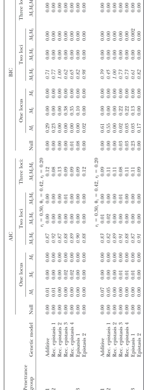
TABLE 5
Simulation 1: proportion of times the model was selected for specified criteria (AIC, BIC) for the null model (no loci) and the one-, two-, three-, and four-locus models
AIC BIC
Penetrance Genetic One Two Three Four One Two Three Four
group model Null locus loci loci loci Null locus loci loci loci
r1⫽0.20,1⫽0.20,r2⫽0.20,2⫽0.20,r3⫽0.20
1 Additive 0.00 0.00 0.57 0.31 0.10 0.03 0.00 0.02 0.97 0.00 0.00 0.00
2 Rec. epistasis 1 0.00 0.00 0.68 0.21 0.09 0.02 0.00 0.03 0.97 0.00 0.00 0.00
3 Epistasis 1 0.00 0.00 0.06 0.89 0.01 0.04 0.00 0.02 0.93 0.07 0.00 0.00
r1⫽0.20,1⫽0.50,r2⫽0.20,2⫽0.50,r3⫽0.20
1 Additive 0.00 0.001 0.44 0.47 0.06 0.03 0.00 0.15 0.85 0.00 0.00 0.00
2 Rec. epistasis 1 0.00 0.00 0.57 0.34 0.08 0.02 0.00 0.04 0.96 0.00 0.00 0.00
3 Epistasis 1 0.01 0.01 0.11 0.83 0.02 0.02 0.00 0.65 0.29 0.06 0.00 0.00
For incorrect models, proportions are the proportion of all possiblet-locus models. The correct model is in italics and the proportion of other three-locus models selected is in regular type. One thousand individuals, 1000 replicates, and three loci were used.Midenotes the marker at locusiandGidenotes BTL locusi,ri is the recombination betweenMiandGi, andiis
the recombination betweenMiandMi⫹1(see simulated map in Figure 1).
the time (see Table 4). This is intuitively logical, since resulted in a higher likelihood of choosing the correct model. AIC tended to select models of too high dimen-the distance between dimen-the BTL and dimen-the marker increases,
and the effect of the penalty for the BIC is more severe sion. The behavior of the AIC was dramatically different between simulations 1 and 2 (see Tables 4 and 6). The than the effect of the penalty for the AIC, making the
BIC more sensitive than AIC to recombination distance. BIC performed similarly in genetic models from group 1 and group 2 while the performance of the BIC in a
Simulation 2: For simulation 2, the focus was on a
subset of genetic models, one from each of the pene- genetic model from group 3 was affected by the addi-tional marker. This change is not nearly as dramatic as trance groups where a large number of extra markers
were included. This simulation provides an opportunity the change for the AIC. However, for the BIC, the ge-netic model affected whether the two-BTL model that to examine the performance of the AIC and BIC in a
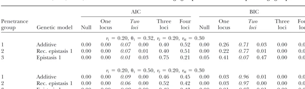
more realistic data analytic setting. In these simulations, included the simulated BTL was selected or not. For example, for the genetic model epistasis 1 from group the BIC far outperformed the AIC (see Table 6) and
TABLE 6
Simulation 2: proportion of times the model was selected for specified criteria (AIC, BIC) for the null model (no loci) and the one-, two-, three-, and four-locus models with 10 linkage groups with 5–20 markers per linkage group
AIC BIC
Penetrance One Two Three Four One Two Three Four
group Genetic model Null locus loci loci loci Null locus loci loci loci
r1⫽0.20,1⫽0.32,r2⫽0.20,rM⫽0.30
1 Additive 0.00 0.00 0.07 0.00 0.40 0.52 0.00 0.26 0.71 0.03 0.00 0.00
2 Rec. epistasis 1 0.00 0.00 0.07 0.01 0.40 0.51 0.00 0.22 0.77 0.01 0.00 0.00
3 Epistasis 1 0.00 0.00 0.01 0.03 0.75 0.21 0.05 0.41 0.07 0.47 0.00 0.00
r1⫽0.20,1⫽0.50,r2⫽0.20,rM⫽0.30
1 Additive 0.00 0.00 0.09 0.00 0.46 0.45 0.00 0.03 0.96 0.01 0.00 0.00
2 Rec. epistasis 1 0.00 0.00 0.06 0.00 0.52 0.42 0.00 0.03 0.97 0.00 0.00 0.00
3 Epistasis 1 0.00 0.00 0.09 0.00 0.48 0.43 0.00 0.01 0.97 0.01 0.00 0.00
The correct model is in italics and the proportion of other two-locus models selected is in regular type. One thousand individuals, 500 replicates, and two loci were used.Midenotes the marker at locusiandGidenotes BTLi,riis the recombination
betweenMi andGi,1is the recombination betweenM1andM2, andrMis recombination between markers on linkage groups
TABLE 7
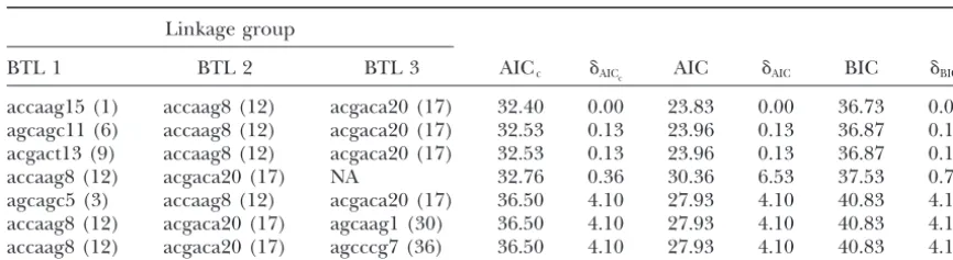
Multiple-locus models with the lowest AICccriterion for each BTL marker name from the linkage
group given with linkage group number in parentheses
Linkage group
BTL 1 BTL 2 BTL 3 AICc ␦AICc AIC ␦AIC BIC ␦BICc
accaag15 (1) accaag8 (12) acgaca20 (17) 32.40 0.00 23.83 0.00 36.73 0.00 agcagc11 (6) accaag8 (12) acgaca20 (17) 32.53 0.13 23.96 0.13 36.87 0.13 acgact13 (9) accaag8 (12) acgaca20 (17) 32.53 0.13 23.96 0.13 36.87 0.13
accaag8 (12) acgaca20 (17) NA 32.76 0.36 30.36 6.53 37.53 0.79
agcagc5 (3) accaag8 (12) acgaca20 (17) 36.50 4.10 27.93 4.10 40.83 4.10 accaag8 (12) acgaca20 (17) agcaag1 (30) 36.50 4.10 27.93 4.10 40.83 4.10 accaag8 (12) acgaca20 (17) agcccg7 (36) 36.50 4.10 27.93 4.10 40.83 4.10
AIC and BIC criteria are also shown.␦iis the difference between the model with the lowest criterion value and the criteria values of the model in that row.
3, the BIC selected a two-BTL model in 54% of the ants were mapped and resulted in 38 linkage groups. The number of AFLP markers in comparison to the cases. However, the correct two-BTL model was selected
in only 7% of the cases. sample size is very large.
Three hundred thirteen single-marker models were
O. mykissdata analysis: Doubled haploids, produced
by androgenesis in the second generation from a cross investigated and the marker with the lowestP-value on each of 38 linkage groups was selected for inclusion in between two clonal lines, were used for a genetic analysis
ofC. shastaresistance. C. shastais a myxozoan parasite the multiple-loci models. Of the 45 segregants, 31 had data for the entire set of 38 selected markers. On the that has a two-stage life cycle. One stage is completed
in a polychaete worm, Manyukia speciosa, and acti- basis of this, we considered the 31 segregants for which complete marker data were available. Using the 38 mark-nospores are released to the water and infect the
intesti-nal tracts of trout, where the organism continues devel- ers on the 31 segregants, all one-locus and two- and three-loci models were investigated (38 one-locus mod-opment, producing myxospores that are evident by
intestinal scrapings. The complete experiment is de- els, 703 two-loci models, and 8436 three-loci models)
using PROC BTL (seeappendixfor PROC BTL). The
scribed in Nichols et al. (2003). Briefly, subyearling
doubled haploids were exposed in live cagesin situto AICccriteria were used for model selection because of
the small sample size. For each of the models the AIC, a pathogen in the Willamette River for 4 days in
Septem-ber 2000. Following the exposure, fish were maintained BIC, and AICcwere calculated and the best models were
selected. The best models were used as input for PROC in flow-through systems at the Center for Disease
Re-search hatchery at Oregon State University. Fish were BTL to estimate the recombination and penetrance pa-rameters.
monitored daily where mortalities were removed,
re-corded, a fin clip taken, and identification number as- The 38 single-BTL models, 703 distinct two-BTL mod-els, and 8436 distinct three-BTL models were fit; 702 of signed for genetic analysis. Evidence ofC. shastaspores
was evaluated from intestinal scrapings of each individ- 703 two-BTL models converged. The best models based on AICc, AIC, and BIC are shown in Table 7. The
differ-ual. The study was terminated 103 days postexposure
and fish still alive were labeled survivors and subse- ence between the lowest model selection criterion value for a particular model and the model in the set with quently euthanized with a lethal dose of anesthetic
(MS-222, Argent Laboratories), fin-clipped, assigned individ- the lowest model selection value is denoted as␦. Of the 8436 models fit, 14% failed to converge, most likely due ual identification numbers, and evaluated for presence
of C. shasta spores in the intestine. Only mortalities to the limited degrees of freedom (sample size). The inclusion of markers accaag8 and acgaca20 on that died fromC. shastainfection, as evidenced by the
presence ofC. shastaspores in the intestines, were used linkage groups OC21 and OC27 is statistically accurate according to the model selection results. Six sets of for genetic analysis of resistance. None of the surviving
fish exhibitedC. shastaspores from intestinal scrapings. estimated recombination and penetrance parameters from the resulting two-locus model are within the range Amplified fragment length polymorphic (AFLP)
mark-ers were employed to genotype individuals for construc- ⫺0.10–1.1 for the penetrance parameters. Estimates for
r1 and r2 were very small, ranging from 0.00 to 0.05.
tion of a genetic linkage map and genetic analysis ofC.
shastaresistance, as previously described (Nicholset al. Estimates forp11ranged from 0.39 to 0.41, forp12ranged
segreg-and forp22ranged from 1.03 to 1.08. The small sample models in our simulations, performance of the BIC de-creases while the AIC remains approximately the same. combined with the observation that none of the
individ-uals with allele 1 of marker accaag8 and allele 2 of Examining these models closely, we see that the varying difficulty can be explained by considering the pene-markeracgaca20survived made the addition of a third
locus unwise from an estimation perspective (marker trance parameters as mixing parameters and examining the relative effect size difference between the loci. class means 11⫽ 0.097,12⫽ 0.00, 21⫽ 0.065, and
22⫽0.26). The goals and results of simulation 2 are markedly
different. Unlinked BTL are easier to identify than linked BTL simply because they are considered inde-DISCUSSION
pendently. This effect can be diminished by expanding the model search space once the best model or set of This article presents a general likelihood for multiple
BTL. The likelihood formulation presented here is simi- models has been selected from among the restricted set. Examining models that increase the number of loci lar to that employed by Yi and Xu (2002) with the
exception that their liability function is replaced by our by adding loci linked to loci already included in the best model will allow for additional opportunities to single penetrance parameter. Since the estimation of
the liability function is computationally challenging, detect linked BTL, while still restricting the model space to a manageable number of loci.
and the methods employed are often sensitive to the
choice of this function, our approach greatly simplifies The comparison between simulation 1 and simulation 2 underscores the main differences among the two crite-the likelihood and corresponding evaluation process.
By choosing one marker per linkage group in a premod- ria examined. The AIC selects the best “approximating” model for the data, and in cases where few markers are eling step, we greatly reduce the model space and avoid
stepwise model selection and complicated searching al- available, these are often the correct selections. In the case of a genome scan, this will result in the addition gorithms. Rather than choosing only markers significant
in the single-locus models or examining all possible of loci, particularly in the case of linked BTL. The BIC will more often choose the right model among a large pairs of loci, the relationships (linkage) between
mark-ers can be exploited to choose the best locus for each set of models when the true model is of relatively low dimension and is included in the set of models to select. linkage group. This reduces the model space and the
impact of model selection upon the subsequent estima- In the case of the genome scan the BIC has a larger penalty and thus more often chooses a model of appro-tion and testing procedures.
While we focus on selection of a single marker in a priate or lower dimension. However, when the number of loci examined is limited, the penalty for the BIC linkage group, the idea of reducing the marker set can
be applied more broadly. For example, in cases where forces models of too low a dimension to be selected.
Bogdan et al. (2004) propose a modification to the
the linkage group may itself be large, the best marker
for some fixed genetic distance may be chosen. Alterna- BIC that accommodates the dimensionality of the BTL application and that could be extended to apply here tively, two or three markers per linkage group may be
selected. and perhaps mitigate this finding.
In the analysis of theO. mykissthere were a fair num-In the first simulation, epistatic models are easier to
select correctly than the strictly additive model. Initially ber of missing marker data. For the purposes of compari-son of the techniques explored in this article, the maxi-this was a surprising result but when a fully additive
model is considered, with the restriction of the parame- mum set of complete data was chosen. This is because one of the main assumptions of both AIC and BIC is a ter space for the penetrance parameters, 0 ⱕ pj ⱕ 1,
the marginal effect of any one locus is small. This is constant sample size. Changing the sample size between models will adversely affect the model selection process what is predicted by Fisher’s infinitesimal model with a
large number of loci. The extension of this idea will be and because of the penalty term, especially with respect to the BIC, changing the criterion between models will true in quantitative traits as well if the range of the trait
values is restricted. In contrast, epistasis restricts the result in changes in the formulation of the likelihood function. As an additional criterion in the premodeling parameters such that several of the penetrances are
equal. The consequence of this is larger marginal effects strategy, one might group markers in the linkage group into a set of best markers and then among those markers of individual loci. This underscores the importance of
fitting models that include epistatic terms as well as choose the marker (or interval) with the most complete data. Furthermore, methods that impute the value of main effects.
The effect of linkage between the BTL changes the missing marker data show promise to reduce the impact of missing marker data. In addition to the missing performance of the selection criteria. For additive
mod-els with recessive epistasis (groups 1 and 2) the influence marker data, the sample size for these data is exceed-ingly small. The size is so small that inferences drawn of linkage among BTL improves model selection. For
ping based on model selection: approximate analysis using the tive conclusions. In general, the small sample correction
Bayesian information criterion. Genetics159:1351–1364. of the AIC (e.g., AICc) is considered preferable com- Bogdan, M., J. K. GhoshandR. W. Doerge, 2004 Modifying the
Schwarz Bayesian information criterion to locate multiple inter-pared to invoking the asymptotic behavior of the AIC
acting quantitative trait loci. Genetics167:989–999. and BIC. Of note is the fact that the three criteria
se-Broman, K. W., andT. P. Speed, 2002 A model selection approach lected the same set of models with similar ranking for the identification of quantitative trait loci in experimental
crosses. J. R. Stat. Soc. Ser. B64:641–656. among models. Examining the set of models that have
Burnham, K. P., and D. R. Anderson, 2002 Model Selection and similar AIC, AICc, and BIC values, it is apparent that
Multimodel Inference: A Practical Information-Theoretic Approach, Ed. linkage groups OC21 and OC27 are a common theme. 2. Springer, Berlin/Heidelberg, Germany/New York.
Carlborg, O., andL. Andersson, 2002 Use of randomization test-This is particularly interesting as linkage group OC27
ing to detect multiple epistatic QTL. Genet. Res.79:175–184. had no significant BTL in the single-marker analysis.
Carlborg, O., L. AnderssonandB. Kinghorn, 2000 The use of This points to the possible identification of an epistatic a genetic algorithm for simultaneous mapping of multiple
inter-acting quantitative trait loci. Genetics155:2003–2010. effect in the absence of a significant main effect for that
Casella, G., and R. L. Berger, 1990 Statistical Inference. Wads-locus. Additional BTL may be located on linkage groups
worth & Brooks/Cole, Pacific Grove, CA.
OC7,OC13,OC15,OC30,OC-a, and OC-b, but the joint Coffman, C. J., R. W. Doerge, M. L. WayneandL. M. McIntyre, 2003 Intersection tests for single marker QTL analysis can be estimation of parameters in models of this dimension
more powerful than two marker QTL analysis. BMC Genet.4:
for this small sample size is not recommended.
10 (http://www.biomedcentral.com/1471-2156/4/10). The typical treatment of binary traits has restricted Cohen, J., 1988 Statistical Power Analysis for the Behavioral Sciences, Ed.
2. Lawrence Earlbaum Associates, Hilldale, NJ. the use of these data to single-marker analyses. What
Doerge, R. W., 2001 Mapping and analysis of quantitative trait loci we propose here is to acknowledge the full depth of
in experimental populations. Nat. Rev. Genet.3:43–52. binary traits by allowing a modeling strategy that accom- Falconer, D. S., andT. F. C. Mackay, 1996 Introduction to
Quantita-tive Genetics, Ed. 4. Longman, Essex, UK. modates the potential for epistasis while being aware of
Gauderman, W. J., andD. C. Thomas, 2001 The role of interacting the computational challenges that are present in
high-determinants in the localization of genes, pp. 393–412 inAdvances dimensional model spaces. By changing the parameter- in Genetics, Vol. 42: Genetic Dissection of Complex Traits, edited by
D. C.Raoand M. A.Province. Academic Press, San Diego. ization of the likelihood function to include marker
Haley, C., and S. Knott, 1992 A simple regression method for class means, the estimation of penetrance can be
ob-mapping quantitative trait loci in line crosses using flanking mark-tained. We implement a grid search technique to obtain ers. Heredity69:315–324.
Harrell, F. E., 2001 Regression Modeling Strategies With Applications the solution. There are other potential solutions to this
to Linear Models, Logistic Regression, and Survival Analysis. Springer, system of nonlinear equations, but these present a
com-New York.
plex numerical problem that is a subject of future work. Hartl, D., andE. Jones, 2001 Genetics: Analysis of Genes and Genomes. Jones & Bartlett, Sudbury, MA.
We have provided an easily accessible procedure in SAS
Holland, J. B., V. A. Portyanko, D. L. HoffmanandM. Lee, 2002 that allows multiple-BTL mapping under a wide range
Genomic regions controlling vernalization and photoperiod re-of strategies for the purpose re-of providing a tool that sponses in oat. Theor. Appl. Genet.105:113–126.
Jannink, J., andR. Jansen, 2001 Mapping epistatic quantitative trait scientists can use with ease and flexibility.
loci with one-dimensional genome searches. Genetics157:445– Even though specific model selection criteria (BIC,
454.
AIC, and AICc) are employed to evaluate the models Jansen, R. C., 1992 A general mixture model for mapping quantita-tive trait loci by using molecular markers. Theor. Appl. Genet. that result from the model selection procedure
pro-85:252–260. posed, other criteria could easily be used in conjunction
Jansen, R. C., 1993 Interval mapping of multiple quantitative trait with the premodeling strategy proposed. The optimal loci. Genetics135:205–211.
Jansen, R. C., andP. Stam, 1994 High resolution of quantitative criterion for model selection is an open and exciting
traits into multiple loci via interval mapping. Genetics136:1447– area of research. In the situation presented here the
1455.
issue is further complicated by constraining the parame- Kao, C.-H., Z-B. ZengandR. D. Teasdale, 1999 Multiple interval mapping for quantitative trait loci. Genetics152:1203–1216. ter space, which in turn makes proper evaluation of
Kilpikari, R., andM. J. Sillanpa¨a¨, 2003 Bayesian analysis of multilo-the correct model choice more difficult than it may
cus association in quantitative and qualitative traits. Genet.
Epide-otherwise appear. miol.25:122–135.
Kutner, M. H., C. J. Nachtsheim, J. NeterandW. Li, 2004 Applied This work is supported by National Science Foundation grant DBI
Linear Statistical Models, Ed. 5. McGraw-Hill Irwin, New York. 98-08026/00-96044 (L.M.M., C.J.C., R.W.D.), National Institutes of
Lander, E. S., andD. Botstein, 1989 Mapping Mendelian factors Health grants NIA-AG16996 (L.M.M.) and 2G12RR003048 (L.M.M.), underlying quantitative traits using RFLP linkage maps. Genetics U.S. Department of Agriculture (USDA) grant 98-35300-6173 121:185–199.
(R.W.D.), USDA-Initiative for Future Agriculture and Food Systems Lynch, M., andB. Walsh, 1998 Genetics and Analysis of Quantitative grant N0014-94-1-0318 (R.W.D., L.M.M.), and a Veterans Affairs Traits. Sinauer Associates, Sunderland, MA.
Mallow, C. L., 1973 Some comments on Cp. Technometrics 12:
Health Services Research Postdoctoral Fellowship (C.J.C.).
591–612.
McIntyre, L. M., C. J. CoffmanandR. W. Doerge, 2001 Detection and localization of a single binary trait locus in experimental populations. Genet. Res.78:79–92.
LITERATURE CITED
Nichols, K., J. BartholomewandG. H. Thorgaard, 2003 Map-ping multiple genetic loci associated withCeratomyxa shasta
resis-Akaike, H., 1973 Information theory as an extension, pp. 267–281
inSecond International Symposium on Information Theory, edited by tance inOncorhynchus mykiss.Dis. Aquat. Org.56(2): 145–154.
Ott, J., 1991 Analysis of Human Genetic Linkage. Johns Hopkins Uni-B.Petrovand F.Csaki. Akademiai Kiado, Budapest.